Packet delay in models of data networks

1 Introduction

Importance of packet-switched data networks in contemporary society cannot be overestimated. In an attempt to understand their complex dynamics, several simplified models have been proposed in recent years [5, 7, 13, 14, 16, 20]. The construction of these models have been inspired by successful and well established in physics methodologies of particle systems, cellular automata and lattice gas cellular automata. The application of these methodologies in the context of data networks provides a promising alternative approach. Even though some of these models are simplistic, they can be expanded and modified to incorporate various realistic aspects of data networks. Additionally, these models are not only amenable to computer simulations but also to obtaining analytical results.

One of the interesting questions which needs to be addressed in the context of these models is an issue of influence of the randomness present in the routing algorithm on the network’s dynamics and its effects on the performance of the network.

In [13] we investigated a model in which packets are routed according to a table stored locally at each node. If the table includes all other nodes of the network, such an algorithm is called full table routing algorithm. However, if only nodes closer than $m$ links away are present in the table (partial table routing), packets with a destination address not present in the table are forwarded to a randomly selected nearest neighbour node. This introduces certain amount of randomness or noise into the system, and as a result, the delay changes. By delay we mean the time required for a packet to reach its destination.

In this work, we will investigate how the delay experienced by a single packet, when no other packets are present, depends on the degree of randomness in the routing scheme. While interactions with other packets will obviously strongly influence the delay, in [13] we found that the delay experienced by a single packet is an important parameter characterizing the network. For example, simulation experiments reported in [13] seem to indicate that in many cases the critical load is inversely proportional to the single packed delay. In an attempt to gain some insight into properties of this important parameter, we will derive analytical estimates for the single packet delay and compare it with direct simulations. Finally, we will discuss how these results affect scalability of the proposed network model.

2 Network Models Definitions

Detailed description of the network model is given in [13]. Here, we summarize only its main features. The purpose of the network is to transmit messages from points of their origin to their destination points. In our model, we will assume that the entire message is contained in a single “capsule” of information, which, by analogy to packet-switching networks, will be simply called a packet. In a real packet-switching network, a single packet carries the information “payload”, and some additional information related to the internal structure of the network. We will ignore the information “payload” entirely, and assume that the packet carries only two pieces of information: time of its creation and the destination address.

Our simulated network consists of a number of interconnected nodes. Each node can perform two functions: of a host, meaning that it can generate and receive messages, and of a router (message processor), meaning that it can store and forward messages. Packets are created and moved according to a discrete time parallel algorithm. The structure of the considered networks and the update algorithm will be described in subsections which follow.

2.1 Connection Topology

In this paper, we will consider a connection topology in a form of a two-dimensional square lattice with periodic boundary conditions ${\mathcal{L}^{p}}$. The network hosts and routers are located at nodes of the lattice $\mathcal{L}^{p}$. The position of each node on a lattice $\mathcal{L}^{p}$ is described by a discrete space variable $\mathbf{r}$, such that

$$\mathbf{r}=i\mathbf{c}_{x}+j\mathbf{c}_{y},$$ (1)

where $\mathbf{c}_{x},\mathbf{c}_{y}$ are Cartesian unit vectors, and $i,j=1,\ldots,L$. The value of $L$ gives a number of nodes in the horizontal and vertical direction of the lattice $\mathcal{L}^{p}$. We denoted by $C(\mathbf{r})$ the set of all nodes directly connected with a node $\mathbf{r}$. For each $\mathbf{r}\in$ $\mathcal{L}^{p}$, the set $C(\mathbf{r})$ is of the form

$$C(\mathbf{r})=\{\mathbf{r}-\mathbf{c}_{x},\mathbf{r}+\mathbf{c}_{x},\mathbf{r}-\mathbf{c}_{y},\mathbf{r}+\mathbf{c}_{y}\}.$$ (2)

In this case, the node $\mathbf{r}$ is connected with its four nearest neighbours. In the networks considered here, each node maintains a queue of unlimited length where the arriving packets are stored. Packets stored in queues, at individual lattice nodes, must be delivered to their destination addresses. To assess how far a given packet is from its destination, we introduce the concept of distance between nodes. We will use periodic “Manhattan” metric to compute the distance between two nodes ${\mathbf{r}}_{1}=(i_{1},j_{1})$ and ${\mathbf{r}}_{2}=(i_{2},j_{2})$:

$$d_{PM}({\mathbf{r}}_{1},{\mathbf{r}}_{2})=L-\left||i_{2}-i_{1}|-\frac{L}{2}\right|-\left||j_{2}-j_{1}|-\frac{L}{2}\right|.$$ (3)

2.2 Update Algorithms

The dynamics of the networks are governed by the parallel update algorithms similar to the algorithm used in [16]. We start with an empty queue at each node, and with discrete time clock $k$ set to zero. Then, the following actions are performed in sequence:

1. At each node, independently of the others, a packet is created with probability $\lambda$. Its destination address is randomly selected with uniform probability distribution among all other nodes in the network. The newly created packet is placed at the end of the queue.

2. At each node, one packet (or none, if the local queue is empty) is picked up from the top of the queue and forwarded to one of its neighboring sites according to a one of the routing algorithms to be described below. Upon arrival, the packet is placed at the end of the appropriate queue. If several packets arrive to a given node at the same time, then they are placed at the end of the queue in a random order. When a packet arrives to its destination node, it is immediately destroyed.

3. $k$ is incremented by 1.

This sequence of events, which constitutes a single time step update, is then repeated arbitrary number of times. The state of the network is observed after sub-step 3, before clock increase and repetition of sub-step 1. In order to explain the routing algorithms mentioned in sub-step 2, we will first describe one of its simplified versions.

Let us assume that we measure distance using metric $d_{PM}$. To decide where to forward a packet located at a node $\mathbf{r}$ with the destination address $\mathbf{r}_{d}$, two steps are performed:

1. From sites directly connected to $\mathbf{r}$, we select sites which are closest to the destination $\mathbf{r}_{d}$ of the packet. More formally, we construct a set $A_{\infty}(\mathbf{r})$ such that

   $$A_{\infty}(\mathbf{r})=\{\mathbf{a}\in C(\mathbf{r}):d(\mathbf{a},\mathbf{r}_{d})=\min_{\mathbf{x}\in C(\mathbf{r})}d_{PM}(\mathbf{x},\mathbf{r}_{d})\}$$ (4)

2. From $A_{\infty}(\mathbf{r})$, we select a site which has the smallest queue size. If there are several such sites, then we select one of them randomly with uniform probability distribution. The packet is forwarded to this site. Using a formal notation again, we could say that the packet is forwarded to a site selected randomly and uniformly from elements of a set $B_{\infty}(\mathbf{r})$ defined as

   $$B_{\infty}(\mathbf{r})=\{\mathbf{a}\in A_{\infty}(\mathbf{r}):n(\mathbf{a},k)=\min_{\mathbf{x}\in A_{\infty}(\mathbf{r})}n(\mathbf{x},k)\},$$ (5)

   where $n(\mathbf{x},k)$ is a queue size at a node $\mathbf{x}$ at time $k$.

To summarize, the routing algorithm $\mathbf{R}_{\infty}$ described above sends the packet to a site which is closest to the destination (in the sense of the metric $d_{PM}$), and if there are several such sites, then it selects from them the one with the smallest queue. If there is still more than one such node, random selection takes place. It is clear that each packet routed according to the algorithm $\mathbf{R}_{\infty}$ will travel to its destination along the shortest possible path (shortest in the sense of the metric $d_{PM}$, not necessarily in terms of a number of time steps required to reach the destination). In real networks, this does not always happen. In order to allow packets to take alternative routes, not necessarily shortest path routes, we will introduce a small modification to the routing algorithm $\mathbf{R}_{\infty}$ described above.

The modified algorithm $\mathbf{R}_{m}$, for each node $\mathbf{r,}$ will use instead of the set $A_{\infty}(\mathbf{r})$ a set $A_{m}(\mathbf{r})$ defined as follows. In the construction of the set $A_{m}(\mathbf{r})$ instead of minimizing distance $d_{PM}(\mathbf{x},\mathbf{r}_{d})$ from $\mathbf{x}$ to the destination $\mathbf{r}_{d}$, as it was done in $(\ref{seta})$, we will minimize $\Theta_{m}(d_{PM}(\mathbf{x},\mathbf{r}_{d}))$, where

$$\Theta_{m}(y)=\left\{\begin{array}[]{ll}y,&\mbox{if $y<m$},\\ m,&\mbox{otherwise},\end{array}\right.$$ (6)

for a given integer $m$. Thus, the definition of the set $A_{m}(\mathbf{r})$ is

$$A_{m}(\mathbf{r})=\{\mathbf{a}\in C(\mathbf{r}):\Theta_{m}(d_{PM}(\mathbf{a},\mathbf{r}_{d}))=\min_{\mathbf{x}\in C(\mathbf{r})}\Theta_{m}(d_{PM}(\mathbf{x},\mathbf{r}_{d}))\}.$$ (7)

The above modification is equivalent to saying that nodes which are further than $m$ distance units from the destination are treated by the routing algorithm as if they were exactly $m$ units away from the destination. If a packet is at a node $\mathbf{r}$ such that all nodes directly linked with $\mathbf{r}$ are further than $m$ units from its destination, then the packet will be forwarded to a site selected randomly and uniformly from the subset of $C(\mathbf{r})$ containing the nodes with the smallest queue size in the set $C(\mathbf{r}).$ It can happen that the selected site can be further away from the destination than the node $\mathbf{r}$.

Therefore, introduction of the cutoff parameter $m$ adds more randomness to the network dynamics. One could also say that the destination attracts packets, but this attractive interaction has a finite range $m$: packets further away than $m$ units from the destination are not being attracted.

It is also possible to relate various values of the cutoff parameter $m$ to different types of routing schemes used in real packet-switching networks. Assume that each node $\mathbf{r}$ maintains a table containing all possible values of $d_{PM}(\mathbf{x},\mathbf{r}_{d})$, for all possible destinations $\mathbf{r}_{d}$ and all nodes $\mathbf{x}\in C(\mathbf{r})$. Assume that packets are routed according to this table by selecting nodes minimizing distance, measured in the metric $d_{PM}$, traveled by a packet from its origin to its destination. Such a routing scheme is called table-driven routing [17] and it is equivalent to the routing algorithm $\mathbf{R}_{\infty}$. In this case, construction of the set $A_{\infty}(\mathbf{r})$ would require looking up appropriate entries in the stored table.

Let us now define $D_{max}$ to be the largest possible distance between two nodes in the network. When $m<D_{max}$, then for a given ${\mathbf{x}}$, we need to store values of $d_{PM}({\mathbf{x}},{\mathbf{r}}_{d})$ only for nodes ${\mathbf{r}_{d}}$ which are less than $m$ units of distance away – for all other nodes distance does not matter, since it will be treated as $m$ by the routing algorithm. Hence, at each node $\mathbf{r}$ the routing table to be stored is smaller than in the case when $m=D_{max}$. The routing scheme based on this smaller routing table is called the reduced table routing algorithm [17] and it is equivalent to the routing algorithm $\mathbf{R}_{m}$. In the case when $m=D_{max}$ the routing algorithm $R_{m}=R_{\infty}.$

Finally, when $m=1$, the distances between hosts and destinations are not considered in the routing process of packets. Therefore, there is no need to store any table of possible paths at nodes of the network. This case corresponds to the table-free routing algorithm [17] in which packets are routed randomly. Hence, this algorithm can send packets on circuitous and long routes to their destinations.

3 Single packet delay

One of the quantities characterizing the performance of a network is a packet delay $\tau_{m}$, frequently used in network performance literature [2, 3, 4, 8, 15, 18, 19]. In our case, the delay will be defined as a number of time steps elapsed from the creation of a packet to its delivery to the destination address when the routing algorithm $\mathbf{R}_{m}$ is used. In [13] we found that the free packet delay, or delay experienced by a packet when no other packets are present, strongly determines behavior of the network, in particular transition point to the congested state. Since in the case of a single packet there is no interaction with other packets, mathematical analysis of packet’s dynamics is considerably simpler. This analysis will be performed in what follows.

First of all, let us note that when the routing algorithm $\mathbf{R}_{m}$ is used, and when the packet is further than $m$ units away from its destination address, it performs a random walk until it hits a node which is $m$ units away from the destination, and then it follows the shortest path to the destination. Obviously, several shortest paths might exists, so there is still randomness in the packet’s motion, but every time step its distance from the destination decreases by one unit.

Let us denote by $\tau_{m}(\mathbf{r}_{0},\mathbf{r}_{d})$ the expected delay time experienced by a packet which starts at $\mathbf{r}_{0}$ and has destination address $\mathbf{r}_{d}$. For a lattice with periodic boundary conditions, only relative position of $\mathbf{r}_{0}$ and $\mathbf{r}_{d}$ is important. Therefore, we will choose $\mathbf{r}_{d}$ to be at the origin, and define $\tau_{m}(\mathbf{r}_{0})=\tau_{m}(\mathbf{r}_{0},\mathbf{0})$.

From our discussion of the packet’s motion we conclude that $\tau_{m}(\mathbf{r}_{0})$ is a sum of two parts:

$$\tau_{m}(\mathbf{r}_{0})=\tau_{m,1}(\mathbf{r}_{0})+\tau_{m,2}(\mathbf{r}_{0}),$$ (8)

where $\tau_{m,1}(\mathbf{r}_{0})$ is the expected time for a random walk to hit a node which is $m$ units away from the origin, and $\tau_{m,2}(\mathbf{r}_{0})$ is the expected time to reach the origin starting from the node which is $m$ units away from the origin. We will call $\tau_{m,1}(\mathbf{r}_{0})$ a random part, and $\tau_{m,2}(\mathbf{r}_{0})$ a semi-deterministic part of the delay $\tau_{m}(\mathbf{r}_{0})$.

Obviously, for a single packet in the network

$$\tau_{m,2}(\mathbf{r}_{0})=\Theta_{m}(d_{PM}(\mathbf{r}_{0},\mathbf{0})),$$ (9)

and it is only $\tau_{m,1}(\mathbf{r}_{0})$ that needs to be computed (if $m<D_{max}$). It turns out that by modifying the problem slightly, an analytical estimation of $\tau_{m,1}(\mathbf{r}_{0})$ can be obtained.

3.1 Analytical estimation of the expected hitting time for a random walk on a lattice ${\mathcal{L}^{p}}$.

First, we observe that for a random walk which start at $\mathbf{r}_{0}$, $\tau_{m,1}(\mathbf{r}_{0})$ is the expected time of hitting the circle $S_{m}(0,d_{PM})=\{\mathbf{r}\in{\mathcal{L}^{p}}:\ d_{PM}(\mathbf{r},\mathbf{0})\leq m\}$

While the circle $S_{m}(0,d_{PM})$ defined in $d_{PM}$ metric is a natural one to be used in our network model, it is not well suited for the estimation of $\tau_{m,1}(\mathbf{r}_{0})$. In order to carry such estimation, we will replace the circle $S_{m}(0,d_{PM})$ by the circle $S_{m}(0,d_{PE})$ in Euclidean metric, as explained below.

For any two points ${\bf r}_{1}=(x_{1},y_{1})$ and ${\bf r}_{2}=(x_{2},y_{2})$ in ${\mathcal{L}^{p}}$ let us define the Euclidean distance with periodic boundaries between this two points as

$${d_{PE}}({\bf r}_{1},{\bf r}_{2})=\sqrt{(\min\{x_{1}-x_{2},L-(x_{1}-x_{2})\})^{2}+(\min\{y_{1}-y_{2},L-(y_{1}-y_{2})\})^{2}}.$$

Notice that this metric is equivalent to the periodic Manhattan metric $d_{PM}$, in particular

$$\frac{1}{\sqrt{2}}\,d_{PM}({\bf r}_{1},{\bf r}_{2})\leq{d_{PE}}({\bf r}_{1},{\bf r}_{2})\leq d_{PM}({\bf r}_{1},{\bf r}_{2}).$$

For ${\bf r}\in{\mathcal{L}^{p}}$ let us set

$$\|{\bf r}\|={d_{PE}}({\bf r},{\bf 0}).$$

Hence, for any $a>0$, the circle of radius $a$ is the set

$$S_{a}=S_{a}(0,d_{PE})=\{{\bf r}\in{\mathcal{L}^{p}}:\ \|{\bf r}\|\leq a\}.$$

Consider a simple random walk $\{X_{k}\}$, $k=0,1,2,\dots$ on ${\mathcal{L}^{p}}$. Let $T_{R}({\bf r};L)$ be the expected time of hitting the circle $S_{R}$ on a lattice ${\mathcal{L}^{p}}$ when the random walk $\{X_{k}\}$ starts at $X_{0}={\bf r}$.

Theorem 3.1

Suppose that $R(1+\epsilon)<L/4$ and $R<\|{\bf r}\|<L/4$. If the random walk $\{X_{k}\}$ starts at ${\bf r}$ then there exist a constant $C=C(\epsilon)>0$ such that

$$T_{R}({\bf r},L)\geq CL^{2}\log\left(\frac{\|{\bf r}\|}{R}\right)\left[1+O\left(\frac{1}{L}+\frac{1}{R^{2}\log(\|{\bf r}\|/R)}\right)\right],$$ (10)

where we write $y(x)=O(x)$ whenever $\sup_{x>0}y(x)/x<\infty$.

The proof of this theorem is based on the following lemma. Consider two numbers $a$ and $c$ such that $0<a<c\leq L/2$ and suppose that $X_{0}={\bf r}$ with $\|{\bf r}\|=b\in(a,c)$. Clearly, $S_{a}\subseteq S_{c}$, $X_{0}\in S_{c}$ and $X_{0}\notin S_{a}$. Let $p_{a,c}({\bf r})$ be the probability that the random walk $\{X_{k}\}$ will hit the circle $S_{a}$ before exiting $S_{c}$.

Lemma 3.2

If $f({\bf r})=\log(\|{\bf r}\|^{2}+1)$, then

$$p_{a,c}({\bf r})\leq\frac{f(c)-f(b)}{f(c)-f(a)}=\frac{\log(c/b)+O(1/b^{2})}{\log(c/a)+O(1/a^{2})}.$$

Proof of the Lemma. The proof is conducted in the spirit of [10], the reader can also find in this book the definition of submartingale and stopping time used further in this paper.

Observe that $\xi_{k}=f(X_{k})$ is a submartingale with respect to a filtration ${\cal F}_{k}=\sigma(X_{0},X_{1},\dots,X_{k})$ generated by the random walk $\{X_{k}\}$. Indeed, simple algebra shows that

$$\frac{1}{4}\log((x+1)^{2}+y^{2}+1) + \frac{1}{4}\log((x-1)^{2}+y^{2}+1)+\frac{1}{4}\log(x^{2}+(y+1)^{2}+1)$$

$$+ \frac{1}{4}\log(x^{2}+(y-1)^{2}+1)>\log(x^{2}+y^{2}+1)$$

and therefore

$${\sf{E\,}}(\xi_{k+1}|{\cal F}_{k})\geq\xi_{k}.$$

Let the stopping time

$$\eta=\inf\{k>0:\ X_{k}\in S_{a}\mbox{ or }X_{k}\in{\mathcal{L}^{p}}\backslash S_{c}\}$$

be the first time when the random walk leaves $S_{c}\backslash S_{a}$. Then $\tilde{\xi}_{k}=\xi_{k\wedge\eta}$ is also a submartingale [6], therefore

$${\sf{E\,}}\tilde{\xi}_{k}\geq{\sf{E\,}}\tilde{\xi}_{0}=f(b)$$ (11)

for all $k$. Obviously, $\eta$ is finite a.s., so $\tilde{\xi}_{k}$ converges in $L^{1}$ to $\xi_{\eta}$ [6]. On the other hand, $f(X_{\eta})\leq f(a)$ if the random walk hits $S_{a}$ before ${\mathcal{L}^{p}}\backslash S_{c}$ and $f(X_{\eta})\geq f(c)$ otherwise. Consequently,

$${\sf{E\,}}[f(X_{\eta})\,|\,X_{\eta}\in S_{a}] \leq f(a),$$

$${\sf{E\,}}[f(X_{\eta})\,|\,X_{\eta}\notin S_{c}] \geq f(c).$$

Since $f(a)<f(b)$ and

$${\sf{E\,}}(\xi_{\eta})={\sf{E\,}}f(X_{\eta})={\sf{E\,}}[f(X_{\eta})\,|\,X_{\eta}\in S_{a}]p_{a,c}({\bf r})+{\sf{E\,}}[f(X_{\eta})\,|\,X_{\eta}\notin S_{c}](1-p_{a,c}({\bf r})),$$

the inequality (11) yields

$$p_{a,c}({\bf r}) \leq \frac{{\sf{E\,}}[f(X_{\eta})\,|\,X_{\eta}\notin S_{c}]-f(b)}{{\sf{E\,}}[f(X_{\eta})\,|\,X_{\eta}\notin S_{c}]-{\sf{E\,}}[f(X_{\eta})\,|\,X_{\eta}\in S_{a}]}$$

$$\leq \frac{{\sf{E\,}}[f(X_{\eta})\,|\,X_{\eta}\notin S_{c}]-f(b)}{{\sf{E\,}}[f(X_{\eta})\,|\,X_{\eta}\notin S_{c}]-f(a)}\leq\frac{f(c)-f(b)}{f(c)-f(a)}.$$

Using the expansion $\log(a^{2}+1)=2\log a+O(1/a)$ applied to $a$, $b$ and $c$ we conclude the proof of the Lemma. Q.E.D.

Figure 1: Illustration to the proof of the Theorem 3.1

Proof of Theorem 3.1. The proof will proceed in three steps. First, we will obtain the upper bound on the probability of reaching $S_{R}$ prior to leaving $S_{L/2-1}$ when a random walk starts at a point ${\bf r}\in G$ where $G$ is the ring $S_{L/4}\backslash S_{L/4-1}$. Next, we will estimate the expected time of reaching $G$ starting from ${\mathcal{L}^{p}}\backslash S_{L/2-1}$. In the second step, we will show that the expected time of hitting $S_{R}$ when the random walk originates inside $G$ is of order $L^{2}\log(L/2R)$. Finally, we will use the fact that the expected time of hitting $S_{R}$ when the walk originates at some ${\bf r}$ with $R<\|{\bf r}\|<L/4$ is at least as large as the product of the probability of hitting $G$ prior to $S_{R}$ and the expected time of hitting $S_{R}$ starting from $G$.

Step 1.

Let $G=S_{L/4}\backslash S_{L/4-1}$ be the set of lattice points inside the ring of “width” one. Consider for each ${\bf r}\in G$ a simple random walk starting at ${\bf r}$, and a probability $p_{R,L/2-1}({\bf r})$ that the random walk starting at ${\bf r}$ will hit $S_{R}$ before ${\mathcal{L}^{p}}\backslash S_{L/2-1}$. Let $p$ be smallest of these probabilities, that is

$$p=\min_{{\bf r}\in G}p_{R,L/2-1}({\bf r}),$$ (12)

then by Lemma 3.2,

$$p\leq\frac{\log 2+O(1/L)}{\log(L/(2R))+O(1/L+1/R^{2})}.$$

Next, let us show that if the random walk starts in ${\mathcal{L}^{p}}\backslash S_{L/2-1}$, then the minimum of all average times before hitting $G$ is of order $L^{2}$. Indeed, when the random walk hits some ${\bf r}=(x,y)\in G$, then ${d_{PE}}({\bf r})\leq L/4$ and therefore both $|x-L/2|\geq L/4$ and $|y-L/2|\geq L/4$. However, for any ${\bf r}_{1}=(x_{1},y_{1})\notin S_{L/2-1}$ at least one of the values $x_{1}-L/2$ or $y_{1}-L/2$ lies inside the segment $[-(\sqrt{2}-1)L/4-1,(\sqrt{2}-1)L/4+1]$ (see Fig. 1). Consequently, the time in which the simple random walk hits $G$ is stochastically larger than $U$, the random variable representing the time in which one-dimensional simple random walk originating in $x\in[-(2-\sqrt{2})L/4-1,(2-\sqrt{2})L/4+1]$ leaves the segment $[-\lfloor L/4\rfloor,\lfloor L/4\rfloor]$. The expected value of this random variable is known (see [11]) and equals

$$(\lfloor L/4\rfloor)^{2}-x^{2}\geq C_{1}L^{2}$$ (13)

for some constant $C_{1}>0$, because $(2-\sqrt{2})/4<1/4$.

Step 2. Let $\nu=\nu({\bf r})=\inf\{k:\ X_{k}\in S_{R}\}$ denote the first time when the random walk starting at $X_{0}={\bf r}\in G$ hits the circle $S_{R}$. Consider a stopped random walk $\tilde{X}_{k}=X_{k\wedge\nu}$ with $\tilde{X}_{0}=X_{0}$. Set $\eta_{0}=0$ and let

$$\eta_{n}=\inf\{k>\eta_{n-1}:\ \tilde{X}_{k}\in G\mbox{ and }\tilde{X}_{k^{\prime}}\notin S_{L/2-1}\mbox{ for some }k^{\prime}\in(\eta_{k-1},k)\}$$

for $k=1,2,\dots$. Thus, $\eta_{k}$’s are consecutive times at which $\tilde{X}_{k}$ finishes “a loop” from $G$ to $G$ visiting ${\mathcal{L}^{p}}\backslash S_{L/2-1}$ for some time. Since the random walk eventually hits $S_{R}$, only finitely many $\eta_{k}$’s will be defined. According to (12), the random number $N$ of such loops before $X_{k}$ hits ${\mathcal{L}^{p}}\backslash S_{L/2-1}$ is stochastically larger than a geometric random variable $\bar{N}$ with parameter $p$ defined by ${\sf{P}}(\bar{N}\geq n)=(1-p)^{n}$, $n=0,1,2\dots$. The probability that the walk originating in $G$ will visit ${\mathcal{L}^{p}}\backslash S_{L/2}$ but will not visit $S_{R}$, $n$ times in a row is at least $(1-p)^{n}$. Consequently,

$$\eta_{N}=\sum_{i=1}^{N}(\eta_{i}-\eta_{i-1})\geq\sum_{i=1}^{N}U_{i}\geq\sum_{i=1}^{\bar{N}}U_{i},$$

where $\{U_{i}\}$ is a sequence of random variables such that ${\sf{E\,}}(U_{i}\,|\,N)\geq C_{1}L^{2}$ in accordance with (13). Since $\nu({\bf r})>\eta_{N}$, then for any ${\bf r}\in G$ we obtain

$$T_{R}({\bf r},L) = {\sf{E\,}}\nu({\bf r})>{\sf{E\,}}\eta_{N}\geq\sum_{n=1}^{\infty}{\sf{E\,}}(\sum_{i=1}^{n}U_{i}\,|\,\bar{N}=n){\sf{P}}(\bar{N}=n)$$

$$\geq C_{1}L^{2}\sum_{n=1}^{\infty}np(1-p)^{n-1}=\frac{C_{1}L^{2}}{p}\geq C_{2}L^{2}\log\frac{L}{2R}\left[1+O\left(\frac{1}{L}+\frac{1}{R^{2}\log\frac{L}{2R}}\right)\right]$$

where $C_{2}=C_{1}/\log 2$.

Step 3. Now suppose that $R<\|{\bf r}\|<L/4$. By Lemma 3.1, the event $A=\{X_{k}$ reaches $G$ before hitting $S_{R}\}$ has the probability

$$1-p_{R,L/4}({\bf r})\geq\frac{f(\|{\bf r}\|)-f(R)}{f(L/4)-f(R)}=\frac{\log(\|{\bf r}\|/R)+O(1/R^{2})}{\log(L/(4R))+O(1/R^{2})}:=q.$$

Consequently,

$$T_{R}({\bf r},L) = {\sf{E\,}}\nu({\bf r})\geq{\sf{E\,}}(\nu({\bf r})\,|\,A){\sf{P}}(A)\geq q\min_{{\bf r}_{1}\in G}{\sf{E\,}}\nu({\bf r}_{1})$$

$$\geq CL^{2}\log(\|{\bf r}\|/R)\left[1+O\left(\frac{1}{L}+\frac{1}{R^{2}\log(\|r\|/R)}\right)\right]$$

since

$$\frac{\log(L/(4R))}{\log(L/(2R))}\geq\frac{\log(1+\epsilon)}{\log(2+2\epsilon)}>0,$$

and the Theorem is proven. Q.E.D.

Corollary 3.3

Under conditions of Theorem 3.1, if $R$ is fixed while both $\|{\bf r}\|\to\infty$ and $L\to\infty$, then

$$T_{R}({\bf r},L)\geq CL^{2}\log(\|{\bf r}\|/R)[1+o(1)].$$

3.2 The asymptotic behavior of $T_{R}$

Here we will study the case when $L$ is so large, that a simple random walk after appropriate rescaling is close to a Brownian motion $B_{t}$ on a square $\tilde{\cal{L}}=[0,1]^{2}$ with periodic boundary conditions.[12] Let $0<\varepsilon<1$, ${\bf r}\in\tilde{\cal{L}}$ and $\tilde{T}_{\varepsilon}({\bf r})$ be the expected time in which Brownian motion starting from ${\bf r}$ will hit a circle of radius $\varepsilon$. To avoid a trivial answer, we always assume that ${\bf r}$ lies outside of this circle. When the rescaled random walk starting at ${\bf r}$ is close to the Brownian motion [12], then for sufficiently large $L$ and $R$

$$T_{R}({\bf r};L)\approx 2L^{2}\tilde{T}_{R/L}({\bf r}/L).$$ (14)

Therefore, from bounds on $\tilde{T}_{\varepsilon}({\bf r})$ we can deduce the asymptotic behavior of $T_{R}({\bf r},L)$.

It follows from [1], p.109, that the function $\tilde{T}_{\varepsilon}({\bf r})$ is a solution of the PDE on a square with periodic boundaries

$$\Delta\tilde{T} = -2,$$

$$\tilde{T}({\bf r})|_{{\bf r}\in\partial C_{\varepsilon}} = 0,$$

where for any $\varepsilon>0$, $\partial C_{\varepsilon}$ denotes the boundary of a circle of a radius $\varepsilon>0$ around the origin ${\bf 0}$. Here we will not be solving this PDE analytically. We will present estimates of $\tilde{T}$, which follow from a probabilistic nature of the model. The following statement is essential, the idea of its proof comes from [9].

Lemma 3.4

Consider a Brownian motion $B_{t}$ on a plane starting from ${\bf r}\in{\sf{R}}^{2}$, such that $\rho=|{\bf r}|\in(a,b)$ and $0<a<b$. Let $u=u(\rho;a,b)$ be the expected time until $B_{t}$ hits the circle $C_{a}$, excluding the time spent outside the circle $C_{b}$, that is

$$u={\sf{E\,}}\int_{0}^{\nu_{a}}1_{\{|B_{t}|\leq b\}}dt$$

where $\nu_{a}=\inf\{t:\ |B_{t}|\leq a\}$, then

$$u(\rho;a,b)=b^{2}\log\frac{\rho}{a}-\frac{\rho^{2}-a^{2}}{2}.$$ (15)

Proof. For a Brownian motion $B_{t}$ with $B_{0}={\bf r}=(x,y)\in C_{b}$ and $u({\bf r})={\sf{E\,}}\nu({\bf r})$ we define $\nu({\bf r})=\int_{0}^{\nu_{a}}1_{\{|B_{t}|\leq b\}}dt$. Consider a circle of a small radius $\rho_{0}$ around ${\bf r}$. Since $u({\bf r})$ is a constant on $\partial C_{b}$, then from the symmetry of a circle and by Markov Principle

$$u({\bf r}) = \frac{1}{\phi_{2}-\phi_{1}}\int_{\phi_{1}}^{\phi_{2}}u(x+\rho_{0}\cos\phi,y+\rho_{0}\sin\phi)d\phi$$

$$+ \frac{1}{2\pi-\phi_{2}+\phi_{1}}\int_{\phi_{2}}^{\phi_{1}+2\pi}u({\bf r})d\phi+O({\rho_{0}}^{2}).$$

In this equation the angles $\phi_{1}$ and $\phi_{2}$ are defined in such a way that $\phi\in(\phi_{1},\phi_{2})$ corresponds to the points $(x+\rho_{0}\cos\phi,y+\rho_{0}\sin\phi)$ lying inside the circle $C_{b}$ and $\phi\in(\phi_{2},\phi_{1}+2\pi)$ corresponds to the points lying outside of the circle $C_{b}$. Taking a Taylor expansion and letting $\rho_{0}\to 0$ yields

$$\nabla u({\bf r})\cdot{\bf n}({\bf r})|_{{\bf r}\in\partial C_{b}}=0,$$ (16)

where ${\bf n}$ is a unit vector normal to $\partial C_{b}$ at ${\bf r}$. On the other hand, for ${\bf r}$ lying inside the set $\{{\bf r}:\ |{\bf r}|<b\}$ we have

$$\Delta u=-2$$ (17)

(see [9]). Solving PDE (17) with the boundary conditions (16) and the condition $u({\bf r})|_{{\bf r}\in\partial C_{a}}=0$, we obtain (15). Q.E.D.

Now, to get the desired estimates on $\tilde{T}$, observe that the geometry of the model implies

$$u\left(\rho\wedge\frac{1}{2};\varepsilon,\frac{1}{2}\right)\leq\tilde{T}_{\varepsilon}({\bf r})\leq u\left(\rho;\varepsilon,\frac{1}{\sqrt{2}}\right)$$

where $\rho$ is the distance from ${\bf r}$ to $\bf 0$ in Euclidean periodic metric on $\tilde{\cal{L}}$. In particular, using the R.H.S. of this inequality we obtain the following result.

Corollary 3.5

Whenever (14) takes place, $T_{R}({\bf r},L)$ is asymptotically bounded from above by

$$L^{2}\log\frac{\|{\bf r}\|}{R}-(\|{\bf r}\|^{2}-R^{2})+o(L^{2}).$$ (18)

In terms of order, this equation matches closely the lower bound given by (10). This is consistent with our results for the discrete case and not really surprising, since the limit of a random walk is a Brownian motion.

3.3 Numerical results

In order to assess quality of analytical estimates of $T_{R}(\mathbf{r})=T_{R}(\mathbf{r},L)$ obtained in the previous section, we will compare them with values of $T_{R}(\mathbf{r})$ calculated numerically by solving the system of linear equations

$$T_{R}(\mathbf{r})=1+\frac{1}{4}(T_{R}(\mathbf{r}+\mathbf{c}_{x})+T_{R}(\mathbf{r}-\mathbf{c}_{x})+T_{R}(\mathbf{r}+\mathbf{c}_{y})+T_{R}(\mathbf{r}-\mathbf{c}_{y})),$$ (19)

with periodic boundary conditions and $T_{R}(\mathbf{r})=0$ for every $\mathbf{r}\in{\mathcal{L}^{p}}$ such that $d_{PE}(\mathbf{r},\mathbf{0})\leq R$. Figure 2a is a semi-log plot of $T_{R}(\mathbf{r})$

a)

b)

Figure 2: Graphs of (a) $T_{R}(\mathbf{r},50)$ as a function of $||\mathbf{r}||$ for $R=1,5$ and (b) $\tau_{m}(\mathbf{r})$ as a function of $d_{PM}(\mathbf{r},\mathbf{0})$ for $m=1,5$ for a lattice ${\mathcal{L}^{p}}$ with $L=50$. Continuous lines are the least square fits using points with $||\mathbf{r}||\leq 10$.

as a function of $||\mathbf{r}||$ for the lattice $L\times L=50\times 50$ and two values of $R$, $R=1$ and $R=5$. Each lattice node for which $||\mathbf{r}||>R$ is represented by a single point on the graph. One can clearly see that for $||\mathbf{r}||$ smaller than about 10, these points form a straight line, in agreement with estimations (10) and (18).

Once we notice that for every $\mathbf{r}\in{\mathcal{L}^{p}}$ such that $d_{PM}(\mathbf{r},\mathbf{0})=m$ we have

$$\frac{m\sqrt{2}}{2}\leq d_{PE}(\mathbf{r},\mathbf{0})\leq m,$$ (20)

we can obtain the following bounds on $\tau_{m,1}(\mathbf{r})$:

$$T_{m}(\mathbf{r})\leq\tau_{m,1}(\mathbf{r})\leq T_{m\sqrt{2}/2}(\mathbf{r}).$$ (21)

The above relationship is well illustrated in Figure 2b, which shows a graph of $\tau_{m,1}(\mathbf{r})$ as a function of $d_{PM}(\mathbf{r},\mathbf{0})$ for $L=50$ and $m=1,5$. As before, the values of $\tau_{m,1}(\mathbf{r})$ were obtained by solving the system of linear equations

$$\tau_{m,1}(\mathbf{r})=1+\frac{1}{4}(\tau_{m,1}(\mathbf{r}+\mathbf{c}_{x})+\tau_{m,1}(\mathbf{r}-\mathbf{c}_{x})+\tau_{m,1}(\mathbf{r}+\mathbf{c}_{y})+\tau_{m,1}(\mathbf{r}-\mathbf{c}_{y})),$$ (22)

with periodic boundary conditions and $\tau_{m,1}(\mathbf{r})=0$ for every $\mathbf{r}\in{\mathcal{L}^{p}}$ such that $d_{PM}(\mathbf{r},\mathbf{0})\leq m$. In the aforementioned figure, the points close to the origin do not lie on a straight line, but lie in an area bounded by two straight lines, as expected from (21).

4 Average delay

In a network model investigated in [13], packets were created at each node with a destination address randomly selected among all nodes of the lattice. A useful quantity characterizing delay experienced by packets under such circumstances is an average delay $\overline{\tau}_{m}$, defined as

$$\overline{\tau}_{m}=\frac{1}{L^{2}}\sum_{\mathbf{r}\in{\mathcal{L}^{p}}}\tau_{m}(\mathbf{r}).$$ (23)

Similarly as in (8), we can write the average delay $\overline{\tau}_{m}$ as a sum of the average random and the average semi-deterministic parts, denoted by $\overline{\tau}_{m,1}$ and $\overline{\tau}_{m,2}$, respectively.

Using (9), we will calculate the average semi-deterministic part of the average delay. First, let us define $N(k)$ to be a number of sites $\mathbf{r}\in{\mathcal{L}^{p}}$ such that $d_{PM}(\mathbf{r},\mathbf{0})=k$, $0\leq k\leq L$. Then we can write $\overline{\tau}_{m,2}$ as

$$\overline{\tau}_{m,2}=\frac{1}{L^{2}}\sum_{\mathbf{r}\in{\mathcal{L}^{p}}}\tau_{m,2}(\mathbf{r})=\frac{1}{L^{2}}\sum_{k=0}^{L}N(k)\Theta_{m}(k).$$ (24)

For simplicity, and without much loss of generality, in what follows we will assume that $L$ is even. It is straightforward to establish that for even $L$

$$N(k)=\left\{\begin{array}[]{ll}1&\mbox{if $k=0$}\\ 4k&\mbox{if $0<k<L/2$}\\ 2L-2&\mbox{if $k=L/2$}\\ 4(L-k)&\mbox{if $L/2<k<L$}\\ 1&\mbox{if $k=L$}\end{array}\right.$$ (25)

which can written in a more compact form as

$$N(k)=\delta_{0,k}+\delta_{L,k}-2\delta_{L/2,k}+2L-|4k-2L|,$$ (26)

where $\delta_{i,j}=1$ if $i=j$ and $\delta_{i,j}=0$ otherwise. Using this result and computing the sum in (24) we obtain

$$\overline{\tau}_{m,2}=\left\{\begin{array}[]{ll}{\displaystyle m-\frac{2m^{3}+m}{3L^{2}}},&\mbox{if $m<L/2$}\vspace{.2cm}\\ {\displaystyle\frac{L}{2}-\frac{2(L-m)^{3}+L-m}{3L^{2}}},&\mbox{otherwise.}\end{array}\right.$$ (27)

Since the average semi-deterministic part of the average delay is always smaller than $m$, for small $m$ it will be negligible compared to the random part. Therefore, in the small $m$ regime, we can expect that the leading term in $\overline{\tau}_{m}$ is a linear function of $\log(m)$, according to our analytical estimate from the previous section. Figure 3 shows that it is indeed the case, as illustrated for $L=100$.

Figure 3: Average delay $\overline{\tau}_{m}$ of a free packet as a function of $m$ for a periodic lattice $50\times 50$. The continuous line represents the least squares fit to the first 10 points.

An important observation which can be made from this figure is that $\overline{\tau}_{m}$ stays close to its $m=L$ value ($\overline{\tau}_{L}$=L/2, see eq. 27) when $m$ is close to $L$. This means that making $m$ slightly smaller than $L$ does not increase delay significantly.

5 Network scalability

Every network at some point of its life span needs to be expanded. It is obvious that as the number of nodes increases, the average delay increases as well, since the number of links to be traversed by a given packet becomes larger. However, the increase in delay, is not the only problem encountered when the network expands. Each node $\mathbf{r}$ stores a routing table, which in our model contains routing information for all nodes $\mathbf{x}\in{\mathcal{L}^{p}}$ such that $d_{PM}(\mathbf{r},\mathbf{x})\leq m$. If by $M(m)$ we denote the number of nodes which are up to $m$ links away from a given node, we can say that the memory required to store the routing table is proportional to $M(m)$, which can be readily computed:

$$M(m)=\sum_{k=1}^{m}N(k)=\left\{\begin{array}[]{ll}2m(m+1),&\mbox{if $0<m<L/2$}\vspace{.2cm}\\ L^{2}-2(L-m)(L-m-1)-2,&\mbox{if $L/2\leq m<L$}.\end{array}\right.$$ (28)

Let us now assume that the “cost” of operating of a single node with routing algorithm $\mathbf{R}_{m}$ is given by

$$c(m,a)=\overline{\tau}_{m}+aM(m),$$ (29)

where $a$ is a nonnegative parameter describing the relative cost of memory vs. average delay. This cost function has been introduced to investigate strategies which could minimize both average delay and memory storage requirements at a node. The above form of $c(m,a)$ simply means that the cost is a linear combination of memory used to store the routing table and the average delay experienced by packets. By using this form we want to express the fact that the delay experienced by packets decreases utility of the network, and therefore increases its “cost”.

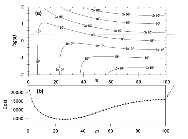
Figure 4: Cost function as a function of $a$ and $m$ shown as a contour plot (a). Part (b) shows the graph of the cost function as a function of $m$ for a fixed value of $a$ ($a=1.58$).

Figure 4 shows how the total cost $c(m,a)$ depends on $m$ and $a$ for $L=50$. For any given value of $a$, one can find the value of $m$ which minimizes the total cost, as shown in Figure 4b.

Obviously, when $a$ is very small, i.e., when the cost of storage is negligible, the total cost is minimal at $m=L$. This means that if the delay alone is taken into consideration, full table routing is always a best choice. In that case, $c(m,a)$ will increase with $L$ as $L^{2}$, meaning that the cost per node will grow proportionally to the number of nodes in the network.

When $a$ is large, the situation is very different. Let us assume, for example, that the value of $a$ is large enough so that the value of $m$ minimizing $c(m,a)$ is small compared to $L$. In this case, the random part of $\overline{\tau}_{m}$ is much larger than the semi-deterministic part, and we can assume that the leading term of $\overline{\tau}_{m}$ has the form

$$\overline{\tau}_{m}\approx\overline{\tau}_{1,m}=AL^{2}\log{\frac{BL}{m}},$$ (30)

where $A$ and $B$ are constants independent of $L$, and therefore

$$c(m,a)\approx AL^{2}\log{\frac{BL}{m}}+2am(m+1).$$ (31)

The above cost function is minimized by

$$m=\frac{\sqrt{a^{2}+4aAL^{2}}}{4a}-\frac{1}{2},$$ (32)

which is an asymptotically linear function of $L$. This means the optimal strategy which should be used to minimize the “cost” of the network is to increase $m$ proportionally to $L$, or in other words, to increase the size of the routing table proportionally to the number of nodes in the network. Note that in this case the cost will still grow with $L$, and for large values of $L$ it will grow like $L^{2}$, similarly as in the case of very small $a$.

6 Conclusion

We have investigated individual packet delay in a model of data networks with table-free, partial table and full table routing. We presented analytical estimates for the average packet delay in a network with small partial routing table and compared them with numerical results. We have also examined the dependence of the delay on the size of a network and on the size of a partial routing table. Assuming the total “cost” of a network with routing algorithm $\mathbf{R}_{m}$ is a linear combination of memory used to store the routing table and the average delay experienced by packets, we discussed consequences of our findings for network scalability. If we are concerned primary with the speed of the network and the memory cost is not important, full table routing is the best choice. On the other hand, if the primary factor influencing the total cost is an amount of memory used to store routing tables, the optimal strategy which should be used to minimize the cost is to keep a size of a routing table proportional to a number of nodes in a network. In that case, the cost per node $c(m,a)$ grows linearly with the size of the network.

Acknowledgements

The authors acknowledge partial financial support from the Natural Sciences and Engineering Research Council (NSERC) of Canada and The Fields Institute for Research in Mathematical Sciences. The discussion of the problem analyzed in Section 3.1 with Mikhail Menshikov was very helpful. One of the authors (H.F.) expresses gratitude to the Department of Mathematics and Statistics, University of Guelph, for hosting him as an NSERC Postdoctoral Fellow.

References

- [1] R. F. Bass. Probabilistic Techniques in Analysis. Springer-Verlag, New York, 1995.
- [2] D. Berteskas and R. Gallagher. Data Networks. Prentice-Hall, Englewood Cliffs, NJ, 1987.
- [3] J. C. Bolot. Characterizing end-to-end packet delay and loss in the internet. J. High Speed Computing, 2:305, 1993.
- [4] M. S. Borella and G. B. Brewster. Measurement and analysis of long-range dependent behavior of internet packet delay. In Proceedings of IEEE INFOCOM, vol. 2, pages 497–504, Piscataway, NJ, 1998. IEEE.
- [5] I. Campos, E. Tarancón, F. Clérot, and L. A. Fernández. Thermal and repulsive traffic flow. Phys. Rev. A, 52(6):5946–5954, 1995.
- [6] Y. S. Chow and H. Teicher. Probability Theory. Springer-Verlag, New York, 1988.
- [7] J. H. B. Deane, C. Smythe, and D. J. Jefferies. Self-similarity in a deterministic model of data transfer. International Journal of Electronics, 80(5):677–691, 1996.
- [8] P. Dhar and R. Ramaswamy. Design of a computer communication network with special reference to throughput and delay considerations. Journal of the Institute of Electronics and Telecommunication Engineers, 28:391–397, 1982.
- [9] E. B. Dynkin and A. A. Yushkevich. Markov Processes: Theorems and Problems. Plenum Press, New York, 1969.
- [10] G. Fayolle, V.A. Malyshev, and M.V. Menshikov. Topics in the Constructive Theory of Countable Markov Chains. Press Syndicate of the University of Cambridge, Cambridge, 1995.
- [11] W. Feller. An Introduction to Probability Theory and Its Applications. Wiley and Sons, Inc., New York, 1968.
- [12] D. Freedman. Brownian Motion and Diffusion. Holden-Day, San Francisco, 1971.
- [13] H. Fukś and A. T. Lawniczak. Performance of data networks with random links. Mathematics and Computers in Simulation, 51:103–119, 1999, arXiv:adap-org/9909006.
- [14] J. Kadirire. Minimising packet copies in multicast routing by exploiting geographical spread. Comput. Commun. Rev., 24(3):47–62, 1994.
- [15] A. Macii, E. Macii, and T. Wolf. Throughput, delay and packet loss analyzes of input buffered atm switch architectures. Systems Analysis Modelling Simulation, 28:69–75, 1997.
- [16] T. Ohira and R. Sawatari. Phase transition in a computer network traffic model. Phys. Rev. E, 58(1):193–195, 1998.
- [17] T. N. Saadawi, M. H. Ammar, and A. E. Hakeem. Fundamentals of Telecommunication Networks. John Wiley and Sons, New York, 1994.
- [18] D. R. Seligman. Traffic routing in a computer network. Comp. Commun., 7:59–64, 1984.
- [19] W. Stallings. High-speed networks: TCP/IP and ATM design principles. Prentice Hall, New Jersey, 1998.
- [20] A. Y. Tretyakov, H. Takayasu, and M. Takayasu. Phase transition in a computer network model. Physica A, 253:315–322, 1998.