Möbius-Invariant Natural Neighbor Interpolation

Abstract

We propose an interpolation method that is invariant under Möbius transformations; that is, interpolation followed by transformation gives the same result as transformation followed by interpolation. The method uses natural (Delaunay) neighbors, but weights neighbors according to angles formed by Delaunay circles.

1 Introduction

An inversion of $\Bbb R^{2}\cup\{\infty\}$ is a bijection generated by a circle, that maps circles to circles and preserves angles between pairs of curves. The circle with center $c$ and radius $r$ gives an inversion as follows: each point $p$ along a ray with origin $c$ is mapped to another point $p^{\prime}$ along the same ray, so that the product of the distances $|cp|$ and $|cp^{\prime}|$ is $r^{2}$. Thus points on the circle remain fixed and the center $c$ maps to $\infty$. The set of products of inversions forms a group, the group of Möbius transformations on Euclidean space $\Bbb E^{2}$.

Möbius transformations arise in data visualization. For example, hyperbolic browsing [5, 6] uses the Poincaré model of the hyperbolic plane to view large graph structures. A change of focus in a hyperbolic browser is given by an isometry of hyperbolic space corresponding to a Möbius transformation of $\Bbb E^{2}$ that maps the unit disk to itself [4]. Brain mapping [3] flattens a convoluted surface by mapping it quasiconformally to a disk; subsequent navigation in the brain map can be accomplished by hyperbolic browsing. For these applications, it is reasonable to ask for computational primitives specially designed for compatibility with Möbius transformations. We previously considered the problem of finding an optimal Möbius transformation for viewing hyperbolic or spherical data [2]. In this paper we give a Möbius-invariant method of extending a function defined only at discrete sample points to a continuous function defined everywhere on their convex hull.

2 Natural Neighbors

Let $S=\{s_{1},s_{2},\dots,s_{n}\}$ be a set of points in $\Bbb E^{2}$, and let $s$ be another point in the convex hull of $S$. Assume we have real- or complex-valued “elevation” $z_{i}$ for each $s_{i}$, and we would like to define an elevation $z=f(s)$ at $s$, such that $f$ is a continuous function of $s$ and $f(s_{i})=z_{i}$.

Natural neighbor interpolation [8] sets $f(s)$ to be a convex combination of the $z_{i}$ values at the natural neighbors (also known as Delaunay or Voronoï neighbors) of $s$. Let $V$ denote the Voronoï cell of $s$ in the Voronoï diagram of $S\cup\{s\})$ (that is, the set of points in $\Bbb E^{2}$ closer to $s$ than to any $s_{i}$), and let $V_{i}$ denote the Voronoï cell of $s_{i}$ in the Voronoï diagram of $S$. Then $f(s)=\sum_{i}w_{i}z_{i}$ where $w_{i}$ is the fraction of $V$ covered by $V_{i}$. See Figure 1(a). Sibson [8] showed that the weights $w_{i}$ act as a sort of local coordinate system for $s$ in the sense that if $s=(x,y)$ and $s_{i}=(x_{i},y_{i})$, then $x_{i}=\sum_{i}w_{i}x_{i}$ and $y_{i}=\sum_{i}w_{i}y_{i}$. Sibson’s theorem also implies that natural neighbor interpolation reconstructs linear functions, that is, if $z_{i}=ax_{i}+by_{i}+c$ for each $i$ and some $a$, $b$, and $c$, then $z=ax+by+c$.

Natural neighbor interpolation is a logical starting point for Möbius-invariant interpolation, because the notion of Voronoï neighbor can be made invariant under Möbius transformations. Two sites $s_{i}$ and $s_{j}$ are extended Voronoï neighbors if there is a circle $C$ through $s_{i}$ and $s_{j}$ bounding either an empty disk or empty disk complement. After an inversion, $C$ or its complement remains empty and thus $s_{i}$ and $s_{j}$ are still neighbors.

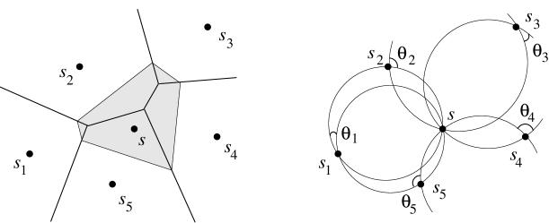
Figure 1: (a) Classical natural neighbor interpolation weights neighbors according to fractions of the area of the Voronoï cell of $s$. (b) Möbius-invariant natural neighbor interpolation weights neighbors according to lune angles.

3 What Weights?

What do we do with the weights $w_{i}$? Area changes under Möbius transformations, so we must find an invariant alternative: angle. The angle most obviously associated with natural neighbor $s_{i}$ is the angle at the lune formed by maximal empty circles, as shown in Figure 1(b). We use the exterior lune angles $\theta_{i}$, because the sum of these angles is fixed: $\sum_{i}\theta_{i}=2\pi$. (One way to see this fact is to perform an inversion that takes $s$ to $\infty$; the exterior lune angles become the exterior angles around the convex hull of the transformed point set.) For invariance, we can simply set $w_{i}$ to be proportional to any function of angle, $w(\theta_{i})$. But is there some especially natural choice for $w()$?

First, we would like the interpolation to be continuous as $s\to s_{i}$, so we require $w(\theta_{i})\to\infty$ as $\theta_{i}\to\pi$. Second, we would like the interpolation to reconstruct some class of functions, analogous to linear functions in Sibson’s method. Harmonic functions (solutions to Laplace’s equation $\nabla^{2}f=0$) would be high on anyone’s wish list, because of numerous applications (heat, electrostatics) and because the family of harmonic functions is itself invariant under Möbius transformations. The values of a harmonic function on a discrete point set, however, do not determine the function, so we cannot hope for a property as strong as Sibson’s theorem. We instead ask for a property that holds only in the limit.

Lemma 1

Let $s_{1},s_{2},\dots,s_{n}$ be a set of points on a circle $C$, and let $\epsilon$ be the maximum angle of arc between a pair of successive $s_{i}$’s. Let $s$ be a point interior to $C$, and let $\theta_{i}$ be the exterior lune angle between $s$ and $s_{i}$ as above. Now let $f$ be a harmonic function defined on the closed disk bounded by $C$. Then as $\epsilon\to 0$, $\sum_{i}\theta_{i}\,f(s_{i})\,\to\,f(s)$.

Proof sketch: There is a Möbius transformation that puts the image of $s$ at the center of the image of circle $C$. Now the harmonic measure of an arc of a disk with respect to the disk center is proportional to its arc angle (see for example [7]). It is not hard to confirm that in the limit of small arcs, the arc angles are the same as the exterior lune angles. Thus $\sum_{i}\,\theta_{i}f(s_{i})$ is the sum over small arcs of harmonic measure times the value of $f()$ at a point in the arc; this sum converges to the limit $\,f(s)$.   

Thus in summary we would like the weighting function $w(\theta_{i})$ to go to infinity as $\theta_{i}\to\pi$ and $w(\theta_{i})/\theta_{i}$ to go to a constant as $\theta_{i}\to 0$. The most obvious choice is to make $w(\theta_{i})$ proportional to $\tan(\theta_{i}/2)$. We normalize the weights so that they sum to one, and thus the actual weights are $w_{i}=(1/W)\tan(\theta_{i}/2)$, where $W=\sum_{i}\tan(\theta_{i}/2)$.

Theorem 1

Natural neighbor interpolation using weights proportional to $\tan(\theta_{i}/2)$ gives a continuous function $f(s)$ that interpolates the elevations at sample points and, in the limit of dense samples on a circle, reconstructs harmonic functions.

Open questions include: Is there a nice $C^{1}$ continuous version? (One idea is to weight by $\tan^{2}(\theta_{i}/2)$, but this loses the harmonic function property.) What about higher-dimensional Möbius-invariant interpolation?

Acknowledgments: We would like to thank Steve Vavasis for helpful conversations.

References

- [1]
- [2] M. Bern and D. Eppstein. Optimal Möbius transformation for information visualization and meshing. 7th Workshop on Algorithms and Data Structures, 2001. LNCS 2125, Springer-Verlag, 14–25.
- [3] M.K. Hurdal, P.L. Bowers, K. Stephenson, D.W.L. Summers, K. Rehm, K. Shaper, and D.A. Rottenberg. Quasi-conformally flat mapping the human cerebellum. http://www.math.fsu.edu/~aluffi/archive/paper98.ps.gz
- [4] B. Iversen. Hyperbolic Geometry. London Math. Soc. Student Texts 25. Cambridge Univ. Press, 1992.
- [5] J. Lamping, R. Rao, and P. Pirolli. A focus + context technique based on hyperbolic geometry for viewing large hierarchies. Proc. ACM Conf. Human Factors in Computing Systems, 1995, pp. 401–408.
- [6] T. Munzner. Exploring large graphs in 3D hyperbolic space. IEEE Comp. Graphics Appl. 18:18–23, 1997.
- [7] C. Pommerenke. Boundary Behaviour of Conformal Maps. Springer-Verlag, 1992.
- [8] R. Sibson. A brief description of natural neighbour interpolation. In Interpreting Multivariate Data, V. Barnett, ed., Wiley, 1981, 21–36.
- [9]