Optimally Cutting a Surface into a Disk

We consider the problem of cutting a set of edges on a polyhedral manifold surface, possibly with boundary, to obtain a single topological disk, minimizing either the total number of cut edges or their total length. We show that this problem is NP-hard, even for manifolds without boundary and for punctured spheres. We also describe an algorithm with running time $n^{O(g+k)}$, where $n$ is the combinatorial complexity, $g$ is the genus, and $k$ is the number of boundary components of the input surface. Finally, we describe a greedy algorithm that outputs a $O(\log^{2}g)$-approximation of the minimum cut graph in $O(g^{2}n\log n)$ time.

1 Introduction

Several applications of three-dimensional surfaces require information about the underlying topological structure in addition to the geometry. In some cases, we wish to simplify the surface topology, to facilitate algorithms that can be performed only if the surface is a topological disk.

Applications when this is important include surface parameterization [20, 46] and texture mapping [3, 44]. In the texture mapping problem, we wish to find a continuous and invertible mapping from the texture, usually a two-dimensional rectangular image, to the surface. Unfortunately, if the surface is not a topological disk, no such map exists. In such a case, the only feasible solution is to cut the surface so that it becomes a topological disk. (Haker et al. [26] present an algorithm for directly texture mapping models with the topology of a sphere, where the texture is also embedded on a sphere.) Of course, when cutting the surface, one would like to find the best possible cut under various considerations. For example, one might want to cut the surface so that the resulting surface can be textured mapped with minimum distortion [20, 25, 46]. To our knowledge, all previous approaches for this cutting problem either rely on heuristics with no quality guarantees [25, 45, 48] or require the user to perform this cutting beforehand [20, 44].

Lazarus et al. [37] presented and implemented two algorithms for computing a canonical polygonal schema of an orientable surface of complexity $n$ and with genus $g$, in time $O(gn)$, simplifying an earlier algorithm of Vegter and Yap [55]. Computing such a schema requires finding $2g$ cycles, all passing through a common basepoint in $\mathcal{M}$, such that cutting along those cycles breaks $\mathcal{M}$ into a topological disk. Since these cycles must share a common point, it is easy to find examples where the overall size of those cycles is $\Omega(gn)$. Furthermore, those cycles share several edges and are visually unsatisfying.

For most applications, computing a canonical schema is overkill. It is usually sufficient to find a collection of edges whose removal transforms the surface into a topological disk. We call such a set of edges a cut graph; see Figure 1 for an example. Cut graphs have several advantages. First, they are compact. Trivially, any cut graph contains at most $n$ edges of the surface mesh, much less than any canonical schema in the worst case, although we expect it to be much smaller in practice. Second, it is quite easy to construct a cut graph for an arbitrary polyhedral surface in $O(n)$ time, using a breadth-first search of the dual graph [13], or simply taking a maximal set of edges whose complement is connected [37]. Finally, the cut graph has an extremely simple structure: a tree with $O(g)$ additional edges. As such, it should be easier to manipulate algorithmically than other representations. For example, Dey and Schipper [13] describe fast algorithms to determine whether a curve is contractible, or two curves are homotopic, using an arbitrary cut graph instead of a canonical schema.

Figure 1: A cut graph for a two-holed torus and its induced (non-canonical) polygonal schema.

In this paper, we investigate the question of how find the “best” such cutting of a surface, restricting ourselves to cuts along the edges of the given mesh. Specifically, we want to find the smallest subset of edges of a polyhedral manifold surface $\mathcal{M}$, possibly with boundary, such that cutting along those edges transforms $\mathcal{M}$ into a topological disk. We also consider the weighted version of this problem, where each edge has an arbitrary non-negative weight and we want to minimize the total weight of the cut graph. The most natural weight of an edge is its Euclidean length, but we could also assign weights to take problem-specific considerations into account. For example, if we want to compute a texture mapping for a specific viewpoint, we could make visible edges more expensive, so that the minimum cut graph would minimize the number of visible edges used in the cuts. Our algorithms do not require the edge weights to satisfy the triangle inequality.

We show that the minimum cut graph of any polyhedral manifold $\mathcal{M}$ with genus $g$ and $k$ boundary components can be computed in $n^{O(g+k)}$ time. We also show that the problem is NP-hard in general, even if $g$ or $k$ is fixed. Finally, we present a simple and efficient greedy approximation algorithm for this problem. Our algorithm outputs a cut graph whose weight is a factor $O(\log^{2}g)$ larger than optimal, in $O(g^{2}n\log n)$ time. If $g=0$, the approximation factor is exactly $2$. As a tool in our approximation algorithm, we also describe efficient algorithms to compute shortest and nearly-shortest nontrivial cycles in a manifold; we believe these algorithms are of independent interest.

2 Background

Before presenting our new results, we review several useful notions from topology and describe related results in more detail. We refer the interested reader to Hatcher [29], Munkres [43], or Stillwell [49] for further topological background and more formal definitions. For related computational results, see the recent surveys by Dey, Edelsbrunner, and Guha [11] and Vegter [54].

2.1 Topology

A $2$-manifold with boundary is a set $\mathcal{M}$ such that every point $x\in\mathcal{M}$ lies in a neighborhood homeomorphic to either the plane $\mathrm{I\!R}^{2}$ or a closed halfplane. The points with only halfplane neighborhoods constitute the boundary of $\mathcal{M}$; the boundary consists of zero or more disjoint circles. This paper will consider only compact manifolds, where every infinite sequence of points has a convergent subsequence.

The genus of a 2-manifold $\mathcal{M}$ is the maximum number of disjoint non-separating cycles $\gamma_{1},\gamma_{2},\dots,\gamma_{g}$ in $\mathcal{M}$; that is, $\gamma_{i}\cap\gamma_{j}=\varnothing$ for all $i$ and $j$, and $\mathcal{M}\setminus(\gamma_{1}\cup\cdots\cup\gamma_{g})$ is connected. For example, a sphere and a disc have genus $0$, a torus and a Möbius strip have genus $1$, and a Klein bottle has genus $2$.

A manifold is orientable if it has two distinct sides, and non-orientable if it has only one side. Although many geometric applications use only orientable $2$-manifolds (primarily because non-orientable manifolds without boundary cannot be embedded in $\mathrm{I\!R}^{3}$ without self-intersections) our results will apply to non-orientable manifolds as well. Every (compact, connected) $2$-manifold with boundary is characterized by its orientability, its genus $g$, and the number $k$ of boundary components [21].

A polyhedral $2$-manifold is constructed by gluing closed simple polygons edge-to-edge into a cell complex: the intersection of any two polygons is either empty, a vertex of both, or an edge of both. We refer to the component polygons has facets. (Since the facets are closed, every polyhedral manifold is compact.) For any polyhedral manifold $\mathcal{M}$, the number of vertices and facets, minus the number of edges, is the Euler characteristic $\chi$ of $\mathcal{M}$. Euler’s formula [18] implies that $\chi$ is an invariant of the underlying manifold, independent of any particular polyhedral representation; $\chi=2-2g-k$ if the manifold is orientable, and $\chi=2-g-k$ if the manifold is non-orientable. Euler’s formula implies that if $\mathcal{M}$ has $v$ vertices, then $\mathcal{M}$ has at most $3v-6+6g$ edges and at most $2v-4+4g-k$ facets, with equality for orientable manifolds where every facet and boundary circle is a triangle. We let $n\leq 6v-10+10g-k$ denote the total number of facets, edges, and vertices in $\mathcal{M}$.

The $1$-skeleton $\mathcal{M}_{1}$ of a polyhedral manifold $\mathcal{M}$ is the graph consisting of its vertices and edges. We define a cut graph $G$ of $\mathcal{M}$ as a subgraph of $\mathcal{M}_{1}$ such that $\mathcal{M}\setminus G$ is homeomorphic to a disk. The disk $\mathcal{M}\setminus G$ is known as a polygonal schema of $\mathcal{M}$. Each edge of $G$ appears twice on the boundary of polygonal schema $\mathcal{M}\setminus G$, and we can obtain $\mathcal{M}$ by gluing together these corresponding boundary edges. Finding a cut graph of $\mathcal{M}$ with minimum total length is clearly equivalent to to finding a polygonal schema of $\mathcal{M}$ with minimum perimeter.

Any $2$-manifold has a so-called canonical polygonal schema, whose combinatorial structure depends only on the genus $g$, the number of boundary components $k$, and whether the manifold is orientable. The canonical schema of an orientable manifold is a ${(4g+3k)}$-gon with successive edges labeled

$$x_{1},y_{1},\bar{x}_{1},\bar{y}_{1},\,\dots,x_{g},y_{g},\bar{x}_{g},\bar{y}_{g},\,z_{1},e_{1},\bar{z}_{1},\,\dots,z_{k},e_{k},\bar{z}_{k};$$

for a non-orientable manifold, the canonical schema is a $(2g+3k)$-gon with edge labels

$$x_{1},x_{1},\,\dots,x_{g},x_{g},\,z_{1},e_{1},\bar{z}_{1},\,\dots,z_{k},e_{k},\bar{z}_{k}.$$

Every pair of corresponding edges $x$ and $\bar{x}$ is oriented in opposite directions. Gluing together corresponding pairs in the indicated directions recovers the original manifold, with the unmatched edges $e_{i}$ forming the boundary circles. For a manifold $\mathcal{M}$ without boundary, a reduced polygonal schema is one where all the vertices are glued into a single point in $\mathcal{M}$; canonical schemata of manifolds without boundary are reduced. We emphasize that the polygonal schemata constructed by our algorithms are neither necessarily canonical nor necessarily reduced.

2.2 Previous and Related Results

Dey and Schipper [13] describe an algorithm to construct a reduced, but not necessarily canonical, polygonal schema for any triangulated orientable manifold without boundary in $O(n)$ time. Essentially, their algorithm constructs an arbitrary cut graph $G$ by depth-first search, and and then shrinks a spanning tree of $G$ to a single point. (See also Dey and Guha [12].)

Vegter and Yap [55] developed an algorithm to construct a canonical schema in optimal $O(gn)$ time and space. Two simpler algorithms with the same running time were later developed by Lazarus et al. [37]. The “edges” of the polygonal schemata produced by all these algorithms are (possibly overlapping) paths in the $1$-skeleton of the input manifold. We will modify one of the algorithms of Lazarus et al. to construct short nontrivial cycles and cut graphs.

Very recently, Colin de Verdiére and Lazarus consider the problem of optimizing canonical polygonal schemata [10]. Given a canonical polygonal schema for a triangulated oriented manifold $\mathcal{M}$, their algorithm constructs the shortest canonical schema in the same homotopy class. Surprisingly (in light of our Theorem 3.1) their algorithm runs in polynomial time under some mild assumptions about the input. As a byproduct, they also obtain a polynomial-time algorithm to construct the minimum-length simple loop homotopic to a given path.

Surface parameterization is an extremely active area of research, thanks to numerous applications such as texture mapping, remeshing, compression, and morphing. For a sample of recent results, see [1, 17, 20, 48, 25, 39, 40, 45, 47, 46, 58] and references therein. In most of these works, surfaces of high genus are parameterized by cutting them into several (possibly overlapping) patches, each homeomorphic to a disk, each with a separate parameterization. A recent exception is the work of Gu et al. [25], which computes an initial cut graph in $O(n\log n)$ time by running a shortest path algorithm on the dual of the manifold mesh, starting from an arbitrary seed triangle. Essentially the same algorithm was independently proposed by Steiner and Fischer [48]. Once a surface has been cut into a disk (or several disks), further (topologically trivial) cuts are usually necessary to reduce distortion [25, 45, 47]. Many of these algorithms include heuristics to minimize the lengths of the cuts in addition to the distortion of the parameterization [25, 40, 45], but none with theoretical guarantees.

All of our algorithms are ultimately based on Dijkstra’s single-source shortest path algorithm [14, 51]. Many previous results have used Dijkstra’s algorithm or one of its continuous generalizations [32, 41, 53] to discover interesting topological structures in $2$-manifolds, such as cut graphs [25, 48], small handles (‘topological noise’) [24], texture atlases [40], contour trees [2, 38], and Reeb graphs [30, 48].

3 Computing Minimum Cut Graphs is NP-Hard

In this section, we prove that finding a minimum cut graph of a triangulated manifold is NP-hard. We consider two versions of the problem. In the weighted case, the manifold is assumed to be a polyhedral surface in $\mathrm{I\!R}^{3}$ and we want to compute the cut graph whose total Euclidean length is as small as possible. In the unweighted case, we are compute the cut graph with the minimum number of edges; the geometry of the manifold is ignored entirely.

Both reductions are from the rectilinear Steiner tree problem: Given a set $P$ of $n$ points from a $m\times m$ square grid in the plane, find the shortest connected set of horizontal and vertical line segments that contains every point in $P$. This problem is NP-hard, even if $m$ is bounded by a polynomial in $n$ [23]. Our reduction uses the Hanan grid of the points, which is obtained by drawing horizontal and vertical lines through each point, clipped to the bounding box of the points. At least one rectilinear Steiner tree of the points is a subset of the Hanan grid [28].

Theorem 3.1

Computing the length of the minimum (weighted or unweighted) cut graph of a triangulated punctured sphere is NP-hard.

• First consider the weighted case, where the weight assigned to each edge of the manifold is its Euclidean length. Let $P$ be a set of $n$ points in the plane, with integer coordinates between $1$ and $m$. We construct a punctured sphere in $O(n^{2})$ time as follows. Assume that $P$ lies on the $xy$-plane in $\mathrm{I\!R}^{3}$. We modify the Hanan grid of $P$ by replacing each terminal with a square of width $1/2n$, rotated $45$ degrees so that its vertices lie on the neighboring edges. These squares will form the punctures. We then attach a basin under each face $f$ of the modified Hanan grid, by joining the boundary of $f$ to a slightly scaled copy of $f$ on the plane $z=-n^{2}$. We also attach a basin of depth $n^{2}+1$ to the boundary of the entire modified Hanan grid. The side facets of each basin are trapezoids. The basins are tapered so that adjacent basins intersect only on the modified Hanan grid. Triangulating this surface arbitrarily, we obtain a polyhedral sphere $\mathcal{M}$ with $n$ punctures and overall complexity $O(n^{2})$. See Figure 2.

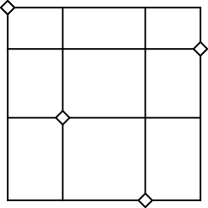
  (a)	(b)	(c)

  Figure 2: (a) A set of integer points. (b) The modified Hanan grid. (c) A cut-away view of the resulting punctured sphere.

Let $G^{*}$ be a minimum weighted cut graph of $\mathcal{M}$. We easily observe that $G^{*}$ contains only “long” edges from the modified Hanan grid and contains at least one vertex of every puncture. Thus, the edges of $G^{*}$ are in one-to-one correspondence with the edge of a rectilinear Steiner tree of $P$.

For the unweighted case, we modify the original $m\times m$ integer grid instead of the Hanan grid. To create a punctured sphere, we replace each terminal point with a small diamond as above. We then fill in each modified grid cell with a triangulation, chosen so that the shortest path between any two points on the boundary of any cell stays on the boundary of that cell; this requires a constant number of triangles per cell. The resulting manifold $\mathcal{M}^{\prime}$ has complexity $O(m^{2})$. By induction, the shortest path between any two points on the modified grid lies entirely on the grid. Thus, any minimal unweighted cut graph of $\mathcal{M}^{\prime}$ contains only edges from the modified grid. It follows that if the minimum unweighted cut graph of $\mathcal{M}^{\prime}$ has $r$ edges, the length of any rectilinear Steiner tree of $P$ is exactly $r$.  ${\square}$

We can easily generalize the previous proof to manifolds with higher genus, with or without boundary, oriented or not, by attaching small triangulated tori or cross-caps to any subset of punctures.

Theorem 3.2

Computing the length of the minimum (weighted or unweighted) cut graph of a triangulated manifold with boundary, with any fixed genus or with any fixed number of boundary components, is NP-hard.

4 Computing Minimum Cut Graphs Anyway

We now describe an algorithm to compute the minimum cut graph of a polyhedral manifold in $n^{O(g+k)}$ time. For manifolds with constant Euler characteristic, our algorithm runs in polynomial time.

Our algorithm is based on the following characterization of the minimum cut graph as the union of shortest paths. A branch point of a cut graph is any vertex with degree greater than $2$. A simple path in a cut graph from one branch point or boundary point to another, with no branch points in its interior, is called a cut path.

Lemma 4.1

Let $\mathcal{M}$ be a polyhedral $2$-manifold, possibly with boundary, and let $G^{*}$ be a minimum cut graph of $\mathcal{M}$. Any cut path in $G^{*}$ can be decomposed into two equal-length shortest paths in $\mathcal{M}_{1}$.

• Let $G$ be an arbitrary cut graph of $\mathcal{M}$, and consider a cut path between two (not necessarily distinct) branch points $a$ and $c$ of $G$. Let $b$ be the midpoint of this path, and let $\alpha$ and $\beta$ denote the subpaths from $b$ to $a$ and from $b$ to $c$, respectively. Note that $b$ may lie in the interior of an edge of $\mathcal{M}_{1}$. Finally, suppose $\alpha$ is not the shortest path from $b$ to $a$ in $\mathcal{M}_{1}$. To prove the lemma, it suffices to show that $G$ is not the shortest cut graph of $\mathcal{M}$.

Let $\alpha^{\prime}$ be the true shortest path from $b$ to $a$. Clearly, $\alpha^{\prime}$ is not contained in $G$. Walking along $\alpha^{\prime}$ from $b$ to $a$, let $s$ be the first vertex whose following edge is not in $G$, and let $t$ be the first vertex in $G$ whose preceding edge is not in $G$. (Note that $s$ and $t$ may be joined by a single edge in $\mathcal{M}\setminus G$.) Finally, let $\sigma^{\prime}\subset\alpha^{\prime}$ be the true shortest path from $s$ to $t$. Equivalently, $\sigma^{\prime}$ is the first maximal subpath of $\alpha^{\prime}$ whose interior lies in $\mathcal{M}\setminus G$. See Figure 3.

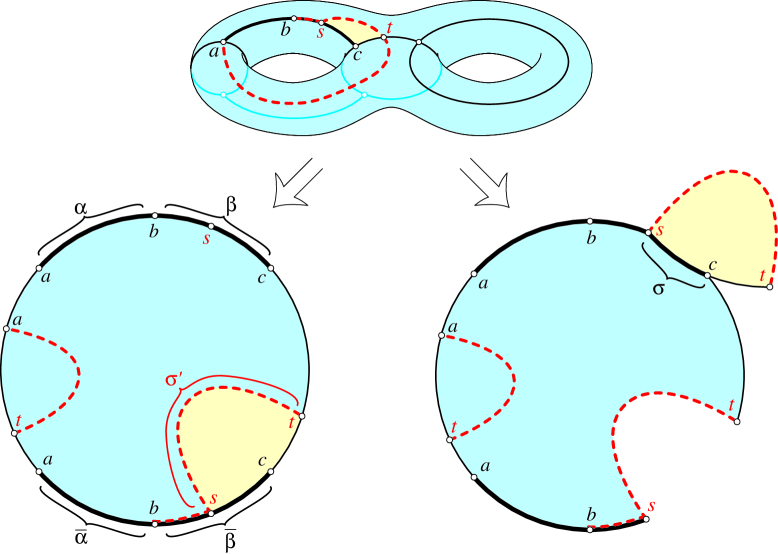
Figure 3: If the dashed path from $a$ to $b$ is shorter than $\alpha$, then the cut graph can be shortened by cutting along $\sigma^{\prime}$ and regluing along $\sigma$.

The subpath $\sigma^{\prime}$ cuts $\mathcal{M}\setminus G$ into two smaller disks. We claim that some subpath $\sigma$ of either $\alpha$ or $\beta$ appears on the boundary of both disks and is longer than $\sigma^{\prime}$. Our claim implies that cutting $\mathcal{M}\setminus G$ along $\sigma^{\prime}$ and regluing the pieces along $\sigma$ gives us a new polygonal schema with smaller perimeter, and thus a new cut graph shorter than $G$. See Figure 3 for an example.

We prove our claim by exhaustive case analysis. First consider the case where the manifold $\mathcal{M}$ is orientable. We can subdivide the entire boundary of the disk $\mathcal{M}\setminus G$ into six paths labeled consecutively $\alpha,\beta,\gamma,\bar{\beta},\bar{\alpha},\delta$. Here, $\bar{\alpha}$ and $\bar{\beta}$ are the corresponding copies of $\alpha$ and $\beta$ in the polygonal schema. Because $\mathcal{M}$ is orientable, $\alpha$ and $\bar{\alpha}$ have opposite orientations, as do $\beta$ and $\bar{\beta}$. Either or both of $\gamma$ and $\delta$ could be empty. See the lower left part of Figure 3. The subpath $\sigma^{\prime}$ can enter the interior of the disk $\mathcal{M}\setminus G$ from four of these six paths ($\alpha$, $\beta$, $\bar{\alpha}$, and $\bar{\beta}$) and leave the interior of the disk through any of the six paths.

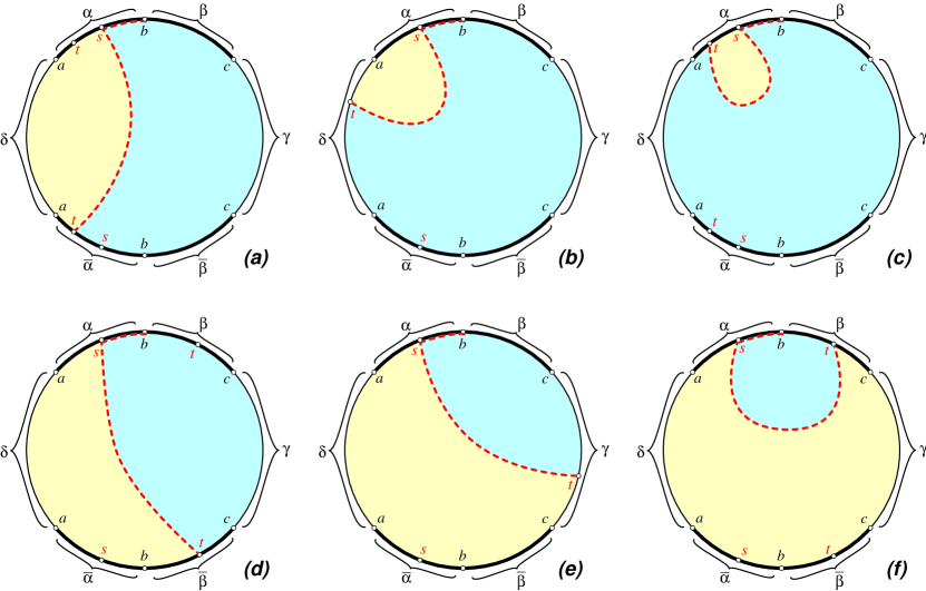
Figure 4: Six cases for the proof of Lemma 4.1 for orientable manifolds; all other cases are reflections of these. In each case, some subpath of $\alpha$ or $\beta$ appears on the boundary of both sub-disks.

Suppose $\sigma^{\prime}$ enters the interior of $\mathcal{M}\setminus G$ from $\alpha$; the other three cases are symmetric. Figure 4 shows the six essentially different ways for $\sigma^{\prime}$ to leave the interior of $\mathcal{M}\setminus G$. In each case, we easily verify that after cutting along $\sigma^{\prime}$, some subpath $\sigma$ of either $\alpha$ or $\beta$ is on the boundary of both disks. Specifically:

1. If $\sigma^{\prime}$ leaves through $\alpha$ or $\bar{\alpha}$ (see Figures 4(c) and 4(a), respectively), then $\sigma$ is the subpath of $\alpha$ from $s$ to $t$. Since both $\sigma$ and $\sigma^{\prime}$ have the same endpoints and $\sigma^{\prime}$ is a shortest path, $\sigma$ must be longer than $\sigma^{\prime}$.

2. If $\sigma^{\prime}$ leaves through $\beta$ or $\bar{\beta}$ (see Figures 4(f) and 4(d), respectively), then $\sigma$ is the subpath of $\beta$ from $b$ to $t$. Indeed, $\rho=\alpha[b,s]\cdot\sigma^{\prime}$ is the shortest path from $b$ to $t$, and as such $\mathopen{|}\sigma^{\prime}\mathclose{|}\leq\mathopen{|}\rho\mathclose{|}<\mathopen{|}\beta[b,t]\mathclose{|}=\mathopen{|}\sigma\mathclose{|}$. (Here $\cdot$ denotes path concatenation, and $\alpha[x,y]$ denotes the subpath of $\alpha$ from $x$ to $y$.)

3. If $\sigma^{\prime}$ leaves through $\gamma$ (see Figure 4(e)), then $\sigma=\beta$. Clearly, $\mathopen{|}\sigma^{\prime}\mathclose{|}<\mathopen{|}\alpha\mathclose{|}=\mathopen{|}\beta\mathclose{|}=\mathopen{|}\sigma\mathclose{|}$.

4. Finally, if $\sigma^{\prime}$ leaves through $\delta$ (see Figure 4(b)), then $\sigma$ is the subpath of $\alpha$ from $a$ to $s$. Clearly, $\mathopen{|}\sigma^{\prime}\mathclose{|}<\mathopen{|}\alpha[s,a]\mathclose{|}\leq\mathopen{|}\sigma\mathclose{|}$.

If $\mathcal{M}$ is non-orientable, the path $\alpha\beta$ could appear either with the same orientation or with opposite orientations on the boundary of the disk $\mathcal{M}\setminus G$. If the orientations are opposite, the previous case analysis applies immediately. Otherwise, the boundary can be subdivided into six paths labeled consecutively $\alpha,\beta,\gamma,\alpha,\beta,\delta$. Without loss of generality, $\sigma^{\prime}$ enters the interior of $\mathcal{M}\setminus G$ from $\alpha$ and leaves through any of these six paths. The six cases are illustrated in Figure 5. Again, we easily verify that in each case, some subpath $\sigma$ of either $\alpha$ or $\beta$ is on the boundary of both disks. We omit further details.  ${\square}$

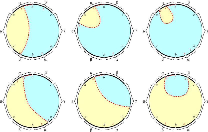
Figure 5: Six additional cases for the proof of Lemma 4.1 for non-orientable manifolds; all other cases are reflections or rotations of these. In each case, some subpath of $\alpha$ or $\beta$ appears on the boundary of both sub-disks.

For any cut graph $G$ of a manifold $\mathcal{M}$, we define the corresponding reduced cut graph $\hat{G}$ as follows. First we remove any topologically trivial cuts; that is, we repeatedly remove any edge with a vertex of degree $1$ that is not on the boundary of $\mathcal{M}$. We then augment the cut graph by adding all the boundary edges of $\mathcal{M}$. Finally, we contract each maximal path through degree-$2$ vertices into a single edge. The resulting reduced cut graph $\hat{G}$ is $2$-edge connected, and each of its vertices has degree at least $3$. Every vertex of $\hat{G}$ is either a branch point or a boundary point of $G$, and every edge of $\hat{G}$ corresponds to either a cut path or a boundary path in $G$. However, in general, not all branch points and cut paths in $G$ are represented in $\hat{G}$.

Lemma 4.2

Let $\mathcal{M}$ be a polyhedral $2$-manifold with genus $g$ and $k$ boundary components. Any reduced cut graph $\hat{G}$ of $\mathcal{M}$ is connected, has between $\max\{1,k\}$ and $4g+2k-2$ vertices, and has between $g+\max\{0,2k-1\}$ and $6g+3k-3$ edges.

• Let $G^{\prime}$ be the cut graph corresponding to $\hat{G}$, after all the trivial cuts have been removed. The boundary of the polygonal schema $\mathcal{M}\setminus G^{\prime}$ can be partitioned into cut paths and boundary paths, each corresponding to an edge in $\hat{G}$. Thus, $\hat{G}$ is connected.

  Let $v$ and $e$ denote the number of vertices and edges in $\hat{G}$, respectively. If any vertex in $\hat{G}$ has degree $d\geq 4$, we can replace it with $d-3$ trivalent vertices and $d-3$ new edges of length zero. Thus, in the worst case, every vertex in $\hat{G}$ has degree exactly $3$, which implies that $3v=2e$. Since $\hat{G}$ is embedded in $\mathcal{M}$ with a single face, Euler’s formula implies that $v-e+1=\chi=2-2g-k$ if $\mathcal{M}$ is orientable, and $v-e+1=\chi=2-g-k$ if $\mathcal{M}$ is non-orientable. It follows that $v\leq 4g+2k-2$ and $e\leq 6g+3k-3$, as claimed.

  On the other hand, $\hat{G}$ has at least one vertex on each boundary component of $\mathcal{M}$, and at least one vertex even if $\mathcal{M}$ has no boundary, so $v\geq\max\{1,k\}$. Thus, Euler’s formula implies that $2-2g-k=v-e+1\geq\max\{1,k\}-e+1$ if $\mathcal{M}$ is orientable, or equivalently, $e\geq 2g+\max\{0,2k-1\}$. Similarly, if $\mathcal{M}$ is non-orientable, Euler’s formula implies that $e\geq g+\max\{0,2k-1\}$.  ${\square}$

Our minimum cut graph algorithm exploits Lemma 4.1 by composing potential minimum cut graphs out of $O(g+k)$ shortest paths. Unfortunately, a single pair of nodes in $\mathcal{M}$ could be joined by $2^{\Omega(n)}$ shortest paths, in $2^{\Omega(g+k)}$ different isotopy classes, in the worst case. To avoid this combinatorial explosion, we can add a random infinitesimal weight $\varepsilon\cdot w(e)$ to each edge $e$. The Isolation Lemma of Mulmuley, Vazirani, and Vazirani [42] implies that if the weights $w(e)$ are chosen independently and uniformly from the integer set $\{1,2,\dots,n^{2}\}$, all shortest paths are unique with probability at least $1-1/n$; see also [9, 34].

We are now finally ready to describe our minimum cut graph algorithm.

Theorem 4.3

The minimum cut graph of a polyhedral $2$-manifold $\mathcal{M}$ with genus $g$ and $k$ boundary components can be computed in time $n^{O(g+k)}$.

• We begin by computing the shortest path between every pair of vertices in $\mathcal{M}$ in $O(n^{2}\log n)$ time by running Dijkstra’s single-source shortest path algorithm for each vertex [14, 31], breaking ties using random infinitesimal weights as described above. Once these shortest paths and midpoints have been computed, our algorithm enumerates by brute force every possible cut graph that satisfies Lemmas 4.1 and 4.2, and returns the smallest such graph.

  Each cut graph is specified by a set $V$ of up to $4g+2k-2$ vertices of $\mathcal{M}$, a set $E$ of up to $6g+3k-3$ edges of $\mathcal{M}$, a trivalent multigraph $\hat{G}$ with vertices $V$, and a assignment of edges in $E$ to edges in $\hat{G}$. Each edge $(v,w)$ of $\hat{G}$ is assigned a unique edge $e\in E$ to define the corresponding cut path in $\mathcal{M}$. This cut path is the concatenation of the shortest path from $v$ to $e$, $e$ itself, and the shortest path from $e$ to $w$. If the midpoint of this cut path is not in the interior of $e$, we declare the cut path invalid, since it violates Lemma 4.1. (Because shortest paths between vertices are unique, the midpoint of any cut path in the minimal cut graph must lie in the interior of an edge.) If all the cut paths are valid, we then check that every pair of cut paths is disjoint, except possibly at their endpoints, and that removing all the cut paths from $\mathcal{M}$ leaves a topological disk.

  Our brute-force algorithm considers $O(n^{4g+2k-2})$ different vertex sets $V$, $O(n^{6g+3k-2})$ different edge sets $E$, at most $\binom{(4g+2k-2)^{2}}{6g+3k-2}$ different graphs $\hat{G}$ for each vertex set, and at most $(6g+3k-2)!$ different assignments of edges in each graph $\hat{G}$ to edges in each edge set $E$. Thus, $n^{O(g+k)}$ potential cut graphs are considered altogether. The validity of each potential cut graph can be checked in $O(n)$ time.  ${\square}$

5 Finding Short Nontrivial Cycles

As a step towards efficiently computing approximate minimum cut graphs, we develop algorithms to compute shortest and nearly-shortest nontrivial cycles in arbitrary $2$-manifolds, possibly with boundary. Although our most efficient approximation algorithm for cut graphs requires only approximate shortest nontrivial cycles on manifolds without boundary, we believe these algorithms are of independent interest.

We distinguish between two type of nontrivial simple cycles. A simple cycle $\gamma$ in $\mathcal{M}$ is non-separating if $\mathcal{M}\setminus\gamma$ has only one connected component. A simple cycle $\gamma$ in $\mathcal{M}$ is essential if it is not contractible to a point or a single boundary cycle of $\mathcal{M}$. Every non-separating cycle is essential, but the converse is not true. Formally, non-separating cycles are homologically nontrivial, and essential cycles are homotopically nontrivial. See Figure 6.

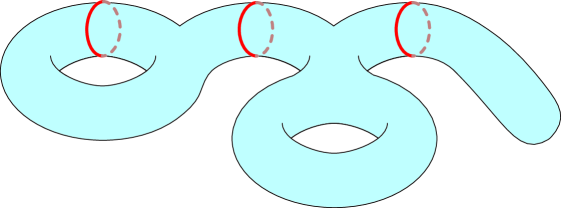
Figure 6: From left to right: non-separating, essential but separating, and trivial cycles on a $2$-manifold.

As can be seen immediately from Figure 6, it is not possible to determine whether a cycle is non-separating, essential, or trivial by examining only a local neighborhood. Dey and Schipper [13] describe an algorithm to determine whether an arbitrary circuit is contractible in $O(n)$ time; their algorithm begins by computing an arbitrary cut graph of the manifold. Fortunately, as we shall see shortly, we can simplify their algorithm considerably when the given cycle is simple.

5.1 Shortest Cycles

We begin by describing how to find the shortest nontrivial cycle through a given vertex. Our algorithm uses a combination of Dijkstra’s single-source shortest path algorithm [14] and a modification of the canonical polygonal schema algorithm of Lazarus et al. [37]. Our algorithm is similar to the approach taken by Guskov and Wood [24] to find and remove small handles from geometric models reconstructed from noisy data; see also [57].

The algorithm of Lazarus et al. builds a connected subset $S$ of a triangulated manifold without boundary, starting with a single triangle and adding new triangles on the boundary of $S$ one at a time. If a new triangle intersects the boundary of $S$ in more than one component, the algorithm checks which of the following three cases holds: (1) $\mathcal{M}\setminus S$ is connected; (2) neither component of $\mathcal{M}\setminus S$ is a disk; or (3) one component of $\mathcal{M}\setminus S$ is a disk. In the final case, the algorithm adds the disk component to $S$ and continues searching the other component of $\mathcal{M}\setminus S$. If we run this algorithm until either case (1) or case (2) holds, the total running time is $O(n)$. See Lazarus et al. [37] for further details.

First we describe a straightforward generalization of the algorithm used by Lazarus to determine the structure of $\mathcal{M}\setminus S$.

Lemma 5.1

Let $\mathcal{M}$ be a connected polyhedral $2$-manifold $\mathcal{M}$ whose genus $g$ and number of boundary components $k$ are known. Any simple cycle $\gamma$ in $\mathcal{M}_{1}$ can be classified as non-separating, essential but separating, or trivial in $O(m)$ time, where $m$ is the complexity of the smaller component of $\mathcal{M}\setminus\gamma$. In particular, if $\gamma$ is non-separating, the running time is $O(n)$.

• We perform two simultaneous depth-first searches, starting from either side of any vertex of $\gamma$. If either search meets a vertex already visited by the other, $\gamma$ is a non-separating cycle. The running time in this case is trivially $O(n)$.

  Conversely, if one search halts without meeting the other, $\gamma$ is a separating cycle. Let $C$ be the smaller component of $\mathcal{M}\setminus\gamma$. To determine whether $\gamma$ is essential, we compute the Euler characteristic and the number of boundary components of $C$, which we denote by $\chi(C)$ and $k(C)$, respectively. (This can be done on the fly during the depth-first search phase.) Let $\chi$ denote the Euler characteristic of $\mathcal{M}$. The cycle $\gamma$ is contractible if and only if one of the following conditions holds.

  • $C$ is a disk, or equivalently, $\chi(C)=1$.

  • $C$ is an annulus, or equivalently, $\chi(C)=0$ and $k(C)=2$.

  • $\mathcal{M}\setminus C$ is a disk, or equivalently, $\chi(C)=\chi-1$. The equivalence follows from the inclusion-exclusion formula $\chi(A\cup B)=\chi(A)+\chi(B)-\chi(A\cap B)$.

  • $\mathcal{M}\setminus C$ is an annulus, or equivalently, $\chi(C)=\chi(\mathcal{M})$ and $k(C)=k(M)$.

  If none of these conditions hold, then $\gamma$ is essential. The total running time if $\gamma$ is a separating cycle is $O(m)$, where $m$ is the complexity of $C$.  ${\square}$

Note that we can simplify this algorithm slightly if the manifold has no boundary, since in that case neither component of $\mathcal{M}\setminus\gamma$ is an annulus. We will use this simplification in our approximate cut graph algorithm.

Lemma 5.2

Let $u$ be a vertex of a polyhedral $2$-manifold $\mathcal{M}$, possibly with boundary. The shortest essential cycle in $\mathcal{M}_{1}$ that contains $u$ can be computed in $O(n\log n)$ time.

• We find the shortest essential cycle through $u$ by simulating a circular wave expanding from $u$. Whenever the wave touches itself, either we have the shortest essential cycle through $u$, or one component of the wave bounds a disk in $\mathcal{M}$ and we can continue expanding the other component.

  We modify the algorithm of Lazarus et al. [37] as follows. First, $S$ is no longer a set of triangles but a more general connected subset of vertices, edges, and facets of $\mathcal{M}$. Initially, $S$ contains only the source vertex $u$. Second, we use Dijkstra’s algorithm to determine the order for edges to be added. We add a facet to $S$ only when all its vertices have been added to $S$, either directly or as part of another facet. We run the algorithm from Lemma 5.1 whenever $S$ is no longer simply connected, that is, when we add a new edge $vw$ with both endpoints on the boundary of $S$. If $\mathcal{M}\setminus S$ is disconnected, we continue only if one component of $\mathcal{M}\setminus S$ is a disk or an annulus, as can be checked using Lemma 5.1. In that case, we add the disk or annulus component of $\mathcal{M}\setminus S$ to $S$, discard the vertices of that component from the Dijkstra priority queue, and continue searching in the other component. If $\mathcal{M}\setminus S$ is connected, or if neither component is a disk or an annulus, we have found the shortest essential cycle through $u$, consisting of the shortest path from $u$ to $v$, the edge $vw$, and the shortest path from $w$ to $u$.

  Dijkstra’s algorithm requires $O(n\log n)$ time. Each time we find a trivial cycle, we spend $O(m)$ time and discard a disk with complexity at least $m$. Thus, the total time spent performing cycle classification and maintaining the wavefront set $S$ is $O(n)$. Thus, the total running time of our algorithm is $O(n\log n)$.  ${\square}$

Running this algorithm once for every vertex of $\mathcal{M}$ immediately gives us the shortest essential cycle.

Corollary 5.3

Let $\mathcal{M}$ be a polyhedral 2-manifold, possibly with boundary. The shortest essential cycle in $\mathcal{M}_{1}$ can be computed in $O(n^{2}\log n)$ time.

A simple modification of our algorithm allows us to find shortest non-separating cycles in the same asymptotic time.

Lemma 5.4

Let $u$ be a vertex of a polyhedral $2$-manifold $\mathcal{M}$, possibly with boundary. The shortest non-separating cycle in $\mathcal{M}_{1}$ that contains $u$ can be computed in $O(n\log n)$ time.

• The only change from the previous algorithm is that if we discover an essential separating cycle, we continue recursively in both components of $\mathcal{M}\setminus S$. The cost of Dijkstra’s algorithm is still $O(n\log n)$, but we now must spend extra time in the cycle-classification algorithm of Lemma 5.1. As before, the total time spent finding trivial cycles is $O(n)$, since we can charge the search time to the discarded components.

  Let $T(n,g)$ denote the total time spent finding separating essential cycles. This function satisfies the recurrence

  $$T(n,g)\leq T(m,h)+T(n-m,g-h)+O(m),$$

  where $m\leq n/2$ is the complexity of the smaller component of $\mathcal{M}\setminus S$ and $h$ is its genus. The base case of the recurrence is $T(n,1)=0$, since every essential cycle on a genus-$1$ surface is non-separating.

  Similar recurrences appear in the analysis of output-sensitive planar convex hull algorithms [5, 8, 33, 56], suggesting that the solution to our recurrence is $T(n,g)=O(n\log g)$. Indeed, we can prove this by induction as follows. Suppose

  $$T(n,g)\leq T(m,h)+T(n-m,g-h)+cm$$

  for some constant $c$. We claim that $T(n,g)\leq cn\lg g$. The inductive hypothesis implies that

  $$T(n,g) \leq cm\lg h+c(n-m)\lg(g-h)+cm$$

  $$\leq\max_{1\leq h\leq g-1}\left(cm\lg h+c(n-m)\lg(g-h)\right)+cm.$$

  A simple application of derivatives implies that the right hand side of this inequality is maximized when $h=mg/n$. Thus,

  $$T(n,g) \leq cm\lg\frac{mg}{n}+c(n-m)\lg\frac{(n-m)g}{n}+cm$$

  $$=cn\lg g+cm\lg m+c(n-m)\lg(n-m)-cn\lg n+cm.$$

  Since $m\leq n/2$ and $n-m\leq n$, we can simplify this inequality to

  $$T(n,g)\leq cn\ln g+cm\lg(n/2)+c(n-m)\lg n-cn\lg n+cm=cn\lg g,$$

  completing the proof.

  Thus, the total time spent in the cycle-classification phase of our algorithm is $O(n\log g)$. Since $g\leq n$, this is dominated by the cost of maintaining the Dijkstra priority queue.  ${\square}$

Corollary 5.5

Let $\mathcal{M}$ be an polyhedral 2-manifold, possibly with boundary. The shortest non-separating cycle in $\mathcal{M}_{1}$ can be computed in $O(n^{2}\log n)$ time.

5.2 Nearly-Shortest Cycles

As we will argue in the next section, computing short nontrivial cycles is the bottleneck in our approximate cut graph algorithm. Fortunately, exact minimum cycles are not necessary for our results. We can speed up our cut graph algorithm, without significantly increasing the approximation factor, by searching for a nontrivial cycle at most twice as long as the shortest. Our approximation algorithm assumes that the manifold $\mathcal{M}$ has no boundary; fortunately, as we shall see in the next section, this is sufficient for our purposes.

Our approximation algorithm works as follows. First, we compute a set of shortest paths (in fact, a cut graph) that intersects every non-separating cycle in the manifold $\mathcal{M}$. Then we contract each shortest path $\pi$ in this set to a point and find the shortest nontrivial cycle through that point, as described by Lemmas 5.2 and 5.4.

Lemma 5.6

Let $\pi$ be a shortest path between two vertices in a polyhedral $2$-manifold $\mathcal{M}$, and let $\gamma^{*}$ be the shortest essential (resp. non-separating) cycle in $\mathcal{M}_{1}$ that intersects $\pi$. In $O(n\log n)$ time, one can compute an essential (resp. non-separating) cycle $\gamma$ in $\mathcal{M}$ such that $\mathopen{|}\gamma\mathclose{|}\leq 2\mathopen{|}\gamma^{*}\mathclose{|}$.

• Let $\mathcal{M}^{\prime}$ be the manifold obtained by contracting the shortest path $\pi$ to a single vertex $v$. Because $\pi$ has no cycles, $\mathcal{M}^{\prime}$ has the same topological type as $\mathcal{M}$. Let $\gamma^{\prime}$ be the shortest essential (resp. non-separating) cycle in $\mathcal{M}^{\prime}$ that passes through $v$. Clearly, $\mathopen{|}\gamma^{\prime}\mathclose{|}\leq\mathopen{|}\gamma^{*}\mathclose{|}$. We can compute this cycle in $O(n\log n)$ time by Lemma 5.2 (resp. Lemma 5.4).

  We construct a cycle $\gamma$ in $\mathcal{M}$ by concatenating two paths $\alpha$ and $\beta$, where $\alpha$ contains the edges of $\gamma^{\prime}$ and $\beta$ is the subpath of $\pi$ between the endpoints of $\alpha$. The sequence of edge contractions that transforms $\mathcal{M}$ to $\mathcal{M}^{\prime}$ also transforms $\gamma^{\prime}$ to $\gamma$. Hence, $\gamma^{\prime}$ is an essential cycle of $\mathcal{M}$. Because $\beta$ is a subpath of a shortest path, $\beta$ is actually the shortest path between the endpoints of $\alpha$, so $\mathopen{|}\beta\mathclose{|}\leq\mathopen{|}\alpha\mathclose{|}=\mathopen{|}\gamma^{\prime}\mathclose{|}$. It follows that $\mathopen{|}\gamma\mathclose{|}=\mathopen{|}\alpha\mathclose{|}+\mathopen{|}\beta\mathclose{|}\leq 2\mathopen{|}\gamma^{\prime}\mathclose{|}\leq 2\mathopen{|}\gamma^{*}\mathclose{|}$.  ${\square}$

This lemma suggests a natural algorithm for finding a short nontrivial cycle: Compute a set of shortest paths that intersect every non-separating cycle (and thus every essential cycle), and then run the algorithm from Lemma 5.6 for each path in this set.

Lemma 5.7

Let $\mathcal{M}$ be a polyhedral $2$-manifold without boundary. In $O(n\log n)$ time, one can compute a set $\Pi$ of $O(g)$ shortest paths on $\mathcal{M}_{1}$ such that every non-separating cycle (and thus every essential cycle) in $\mathcal{M}_{1}$ intersects at least one path in $\Pi$.

• We compute a cut graph $G$ as follows. First we compute a shortest-path tree $T$ from an arbitrary initial vertex $v$ using Dijkstra’s algorithm. We then compute an arbitrary spanning tree $T^{*}$ of the dual of $\mathcal{M}\setminus T$, that is, the graph whose vertices are facets of $\mathcal{M}$ and whose edges join pairs of facets that share a common edge not in $T$. Analysis similar to Lemma 4.2 implies that there are $O(g)$ edges that do not appear in $T$ and whose dual edges to not appear in $T^{*}$. Call this set of unclaimed edges $E$. Let $\Pi$ be the set of $O(g)$ shortest paths from $v$ to the endpoints of $E$; these paths are all in $T$. Finally, let $G=\Pi\cup E^{\prime}$.

  We easily observe that $\mathcal{M}\setminus G$ is a topological disk, so $G$ is a cut graph. It follows that every non-separating cycle in $\mathcal{M}_{1}$ intersects $G$. Since every vertex of $G$ is also a vertex of some path in $\Pi$, every non-separating cycle in $\mathcal{M}_{1}$ intersects at least one path in $\Pi$.  ${\square}$

Notice that this algorithm does not work if $\mathcal{M}$ has a boundary, since the dual graph of $\mathcal{M}\setminus T$ could be disconnected.

Corollary 5.8

Let $\mathcal{M}$ be a polyhedral $2$-manifold with genus $g$ and no boundary, and let $\gamma^{*}$ be its shortest essential (resp. non-separating) cycle. In $O(gn\log n)$ time, one can compute an essential (resp. non-separating) cycle $\gamma$ in $\mathcal{M}_{1}$ such that $\mathopen{|}\gamma\mathclose{|}\leq 2\mathopen{|}\gamma^{*}\mathclose{|}$.

• We construct a set $\Pi$ of $O(g)$ shortest paths, at least one of which is guaranteed to intersect $\gamma^{*}$, as described in the previous lemma. Then for each path $\pi\in\Pi$, we contract $\pi$ to a point and find the shortest nontrivial cycle through that point in $O(n\log n)$ time, as described by Lemma 5.6.  ${\square}$

6 Approximate Minimum Cut Graphs

We now describe a simple polynomial-time greedy algorithm to construct an approximate minimum cut graph for any polyhedral manifold $\mathcal{M}$.

To handle manifolds with boundary, it will be convenient to consider the following simplified form. Given a manifold $\mathcal{M}$ with genus $g$ and $k$ boundary components, the corresponding punctured manifold $(\overline{\mathcal{M}},P)$ consists of a manifold $\overline{\mathcal{M}}$ with the same genus as $\mathcal{M}$ but without boundary, and a set $P$ of $k$ points in $\overline{\mathcal{M}}$, called punctures. To construct $\overline{\mathcal{M}}$, we contract every boundary component of $\mathcal{M}$ to a single point, which becomes one of the punctures in $P$. If any vertex of $\mathcal{M}$ has multiple edges to the same boundary component, $\overline{\mathcal{M}}$ contains only the edge with smallest weight, breaking ties using the Isolation Lemma as above. If $\mathcal{M}$ has no boundary, then $\overline{\mathcal{M}}=\mathcal{M}$ and $P=\varnothing$.

Our goal now is to compute the minimum cut graph of $\overline{\mathcal{M}}$ that touches every puncture in $P$; henceforth, we call this simply the minimum cut graph of $(\overline{\mathcal{M}},P)$. This reduction is motivated by the following trivial observation.

Lemma 6.1

The minimum cut graph of any polyhedral $2$-manifold $\mathcal{M}$ has the same length as the minimum cut graph of $(\overline{\mathcal{M}},P)$.

Our approximation algorithm works as follows. We repeatedly cut along short nontrivial cycles until our surface becomes a collection of punctured spheres, connect the punctures on each component by cutting along a minimum spanning tree, and finally (if necessary) reglue some previously cut edges to obtain a single disk. The resulting cut graph is composed of a subset of the edges of the short nontrivial cycles and all the edges of the minimum spanning forest.

6.1 Using Short Nontrivial Cycles

The first component of our algorithm is a subroutine to compute approximately shortest nontrivial cycles, described by Corollary 5.8. As required by that algorithm, the input manifold $\overline{\mathcal{M}}$ has no boundary; the punctures are completely ignored.

The following argument relates the length of the shortest nontrivial cycles to the length of the minimum cut graph.

Lemma 6.2

Let $G$ be any cut graph of a polyhedral $2$-manifold $\overline{\mathcal{M}}$ with genus $g$ and no boundary. The shortest cycle in $G$ contains $O((\log g)/g)$ of the total length of $G$.

• First consider the reduced cut graph $\hat{G}$, constructed by repeatedly contracting any edge with a vertex of degree less than three, as in Section 4. Every vertex in $\hat{G}$ has degree at least $3$. Without loss of generality, assume that every vertex in $\hat{G}$ has degree exactly $3$, splitting each high-degree vertex into a tree of degree-$3$ vertices if necessary, as in the proof of Lemma 4.2. A straightforward counting argument implies that any trivalent graph whose girth (minimum cycle length) is $c$ must have at least $3\sqrt{2}\cdot 2^{c/2}-2$ vertices if $c$ is odd, and at least $2\cdot 2^{c/2}-2$ vertices if $c$ is even [6]. By Lemma 4.2, $\hat{G}$ has at most $4g-2$ vertices, so $\hat{G}$ must have a cycle $\hat{\gamma}$ with most $2(\lg g+1)=O(\log g)$ edges.

  Starting with $\hat{G}_{0}=\hat{G}$, we inductively define a sequence of reduced graphs $\hat{G}_{1},\hat{G}_{2},\dots$ as follows. For each $i>0$, let $\hat{\gamma}_{i}$ denote the shortest cycle in $\hat{G}_{i-1}$. We obtain $\hat{G}_{i}$ by reducing the graph $\hat{G}_{i-1}\setminus\hat{\gamma}_{i}$, or equivalently, removing the vertices of $\hat{\gamma}_{i}$ and all their edges, and then contracting $\mathopen{|}\hat{\gamma}_{i}\mathclose{|}$ nearby length-$2$ paths to single edges. Our earlier argument implies that each cycle $\hat{\gamma}_{i}$ has at most $2(\lg g+1)$ edges. Thus, for each $i$, we have $\mathopen{|}E(\hat{G}_{i})\mathclose{|}=\mathopen{|}E(\hat{G}_{i-1})\mathclose{|}-6(\lg g+1)$. Lemma 4.2 implies that the original reduced cut graph $\hat{G}$ has at least $g$ edges, so we can repeat this process at least $g/6(\lg g+1)$ times.

  Let $\gamma_{i}$ denote the cycle in the original cut graph $G$ corresponding to $\hat{G}_{i}$. By our construction, $\gamma_{i}$ and $\gamma_{j}$ are disjoint for all $i\neq j$, so we have a set of at least $g/6(\lg g+1)$ disjoint cycles in $G$. At least one of these cycles has length at most $6(\lg g+1)/g=O((\log g)/g)$ times the total length of $G$.  ${\square}$

Since every cycle in the minimum cut graph is non-separating, and therefore essential, we immediately have the following corollary.

Corollary 6.3

For any polyhedral $2$-manifold $\overline{\mathcal{M}}$ with genus $g$ and no boundary, both the length of the shortest non-separating cycle and the length of the shortest essential cycle are at most $O((\log g)/g)$ times the length of the minimum cut graph of $\overline{\mathcal{M}}$.

6.2 Puncture-Spanning Trees

The second component of our cut graph algorithm is a subroutine to compute the minimum puncture-spanning tree of a punctured manifold $(\overline{\mathcal{M}},P)$, that is, the minimum spanning tree of the punctures $P$ in the shortest-path metric of $\overline{\mathcal{M}}_{1}$.

Lemma 6.4

The minimum puncture-spanning tree of any punctured polyhedral $2$-manifold $(\overline{\mathcal{M}},P)$ can be computed in $O(n\log n)$ time.

• We simulate Kruskal’s minimum spanning tree algorithm [36, 51] by adding shortest puncture-to-puncture paths one at a time, in increasing order of length. To compute the shortest paths, we simultaneously propagate wavefronts from all $k$ punctures using Dijkstra’s algorithm. Whenever two wavefronts (i.e., two growing shortest-path trees) collide, we add a new edge to the evolving minimum spanning tree and merge those two wavefronts. To implement this algorithm efficiently, we maintain the wavefronts in a union-find data structure. The resulting running time is $O(n\log n)$.  ${\square}$

This is essentially the algorithm proposed by Takahashi and Matsuyama [50] to compute approximate Steiner trees in arbitrary graphs. The same algorithm was also recently used by Sheffer [45] and by Lévy et al. [40] to compute cut graphs, where surface features with high discrete curvature play the role of punctures.

Lemma 6.5

The length of the minimum puncture-spanning tree of any punctured polyhedral $2$-manifold $(\overline{\mathcal{M}},P)$ is at most twice the length of any cut graph of $(\overline{\mathcal{M}},P)$.

• The minimum Steiner tree of $P$ is the subgraph of $\overline{\mathcal{M}}_{1}$ of minimum total weight that includes every point in $P$. Since any cut graph of $(\overline{\mathcal{M}},P)$ must touch every puncture, no cut graph is shorter than this minimum Steiner tree. On the other hand, the minimum spanning tree of $P$ has at most twice the length of the minimum Steiner tree [35, 50].  ${\square}$

6.3 Analysis

We now have all the components of our greedy cut graph algorithm. At any stage of the algorithm, we have a punctured manifold $(\overline{\mathcal{M}},P)$. Our algorithm repeatedly cuts along a short non-separating cycle of $\overline{\mathcal{M}}$, using Corollary 5.8. This cut creates one or two new boundary circles, which we collapse to new punctures. When the manifold is reduced to a collection of punctured spheres, we cut along the minimum puncture-spanning tree of each component using the algorithm in Lemma 6.4.

Each non-separating cycle cut reduces the genus of $\mathcal{M}$ by $1$. This immediately implies that our algorithm performs exactly $g$ cycle cuts, so the overall running time is

$$g\cdot O(gn\log n)+O(n\log n)=O(g^{2}n\log n).$$

For any graph $X$, let $\mathopen{|}X\mathclose{|}$ denote its total length. Let $G^{*}$ denote the minimum cut graph of $(\overline{\mathcal{M}},P)$. Let $(\overline{\mathcal{M}}_{i},P_{i})$ denote the punctured manifold after $g-i$ cycle cuts have been performed, so $\mathcal{M}_{i}$ has genus $i$, and let $G^{*}_{i}$ denote the minimum cut graph of $\overline{\mathcal{M}}_{i}$, ignoring the punctures $P_{i}$. Since collapsing edges cannot increase the minimum cut graph length, we have $\mathopen{|}G^{*}_{i}\mathclose{|}\leq\mathopen{|}G^{*}_{g}\mathclose{|}\leq\mathopen{|}G^{*}\mathclose{|}$ for all $i$.

Let $\gamma_{i}$ denote the short non-separating cycle of $\mathcal{M}_{i}$ found by Corollary 5.8. (We easily observe that any cut graph of $\overline{\mathcal{M}}_{i}$ must intersect this cycle.) Lemma 6.2 and Corollary 5.8 imply that $\mathopen{|}\gamma_{i}\mathclose{|}\leq O((\log i)/i)\cdot\mathopen{|}G^{*}_{i}\mathclose{|}$ for all $i$ and $j$. Summing over all $g$ cuts, we conclude that the total length of all cycle cuts is at most

$$\sum_{i=1}^{g}O((\log i)/i)\cdot\mathopen{|}G_{i}^{*}\mathclose{|}=O(\log^{2}g)\cdot\mathopen{|}G^{*}\mathclose{|}.$$

Similarly, Lemma 6.5 implies that the minimum puncture-spanning forest has length at most $2\mathopen{|}G^{*}\mathclose{|}$. Finally, regluing previously cut edges to obtain a single disk only reduces the length of the final cut graph. Thus, the final cut graph computed by our algorithm has length at most $O(\log^{2}g)\cdot\mathopen{|}G^{*}\mathclose{|}$.

Theorem 6.6

Given a polyhedral $2$-manifold $\mathcal{M}$ with genus $g$ and $k$ boundary components, an $O(\log^{2}g)$-approximation of its minimum cut graph can be constructed in $O(g^{2}n\log n)$ time.

Cutting along short essential cycles instead of short non-separating cycles leads to exactly the same asymptotic running time and approximation bounds, although the algorithm and its analysis are slightly more complicated. For purposes of analysis, we can divide the algorithm into phases, where in the $i$th phase, we cut along a short essential cycle of every component of the manifold that has genus $i$. Essential cycle cuts can separate the manifold into multiple components, but since each component must have nontrivial topology, the algorithm performs at most $g-1$ separating cuts. At the end of the algorithm, if necessary, we reglue along some previously cut edges to obtain a single topological disk. We refer to the earlier version of this paper for further details [19].

7 Open Problems

We have developed new algorithms to compute exact and approximate minimal cut graphs for manifold surfaces with arbitrary genus and arbitrary boundary complexity. Our approximation algorithm is particularly simple.

Our results suggest several open problems, the most obvious of which is to improve the running times and approximation factors of our algorithms. Is the minimum cut graph problem fixed-parameter tractable [15]? That is, can we compute exact minimum cut graphs in time $f(g,k)\cdot n^{O(1)}$ for some function $f$? The similarity to the Steiner problem offers some hope here, since the minimum Steiner tree of $k$ nodes in an $n$-node graph can be computed in $O(3^{k}n+2^{k}n^{2}+n^{3})$ time [16, 27].

The approximation algorithm of Theorem 6.6 is somewhat indirect. It computes a short cut graph by repeatedly computing a ‘reasonable’ cut graph and then extracting a short nontrivial cycle that interacts with this cut graph. It is natural to conjecture that one can compute such a short cut graph directly, resulting in a faster algorithm. In particular, we conjecture that an approximately minimum cut graph can be computed in $O(gn\log n)$ time.

How well can we approximate the minimum cut graph in nearly-linear time? There are several simple heuristics to compute ’good’ cut graphs in $O(n\log n)$ time, such as the dual shortest-path algorithm used by Gu et al. [25] and by Steiner and Fischer [48], and the algorithm described in the proof of Lemma 5.7. How well do these algorithms approximate the minimum cut graph?

More generally, is there a simple, practical, $O(1)$-approximation algorithm, like the minimum spanning tree approximation of Steiner trees? In fact, it might be that our algorithm provides such an approximation, as our current analysis seems to be far from tight. Unfortunately, the general Steiner tree problem is MAXSNP-hard [4], so an efficient $(1+\varepsilon)$-approximation algorithm for arbitrary $\varepsilon>0$ seems unlikely.

Several authors have pointed out apparent tradeoffs between the quality of parameterizations and the length of the required cut graph; see, for example, Sorkine et al. [47]. How hard is it to compute the (approximately) shortest cut graph required for a parameterization whose distortion is less than some given limit? Conversely, how hard is it to (approximately) minimize the distortion of a parameterization, given an upper bound on the permitted length of the surface cuts? The complexity of these problems clearly depends the which distortion measure is used, but we expect almost any variant of this problem to be NP-hard.

Finally, can our ideas be applied to other useful families of curves on manifolds, such as homology generators (families of $2g$ cycles that intersect in $g$ pairs) and pants decompositions (maximal sets of pairwise disjoint essential cycles [52])?

Acknowledgments. We would like to thank Herbert Edelsbrunner for an enlightening initial conversation. We are also grateful to Noga Alon, Steven Gortler, John Hart, Benjamin Sudakov, Kim Whittlesey, and Zoë Wood for helpful discussions.

References

- [1] P. Alliez, M. Meyer, and M. Desbrun. Interactive geometry remeshing. To appear in Proc. SIGGRAPH ’02, 2002.
- [2] U. Axen and H. Edelsbrunner. Auditory Morse analysis of triangulated manifolds. Mathematical Visualization, 223–236, 1998. Springer-Verlag.
- [3] C. Bennis, J.-M. Vézien, G. Iglésias, and A. Gagalowicz. Piecewise surface flattening for non-distorted texture mapping. Computer Graphics (SIGGRAPH ’91 Proceedings), 237–246, 1991. vol. 25.
- [4] M. Bern and P. Plassman. The Steiner problem with edge lengths and . Inform. Proc. Lett. 32(4):171–176, 1989.
- [5] B. K. Bhattacharya and S. Sen. On a simple, practical, optimal, output-sensitive randomized planar convex hull algorithm. J. Algorithms 25:177–193, 1997.
- [6] N. Biggs. Constructions for cubic graphs with large girth. Elec. J. Combin. 5:A1, 1998.
- [7] J. Blömer. Computing sums of radicals in polynomial time. Proc. 32nd Annu. IEEE Sympos. Found. Comput. Sci., 670–677, 1991.
- [8] T. M. Chan, J. Snoeyink, and C. K. Yap. Primal dividing and dual pruning: Output-sensitive construction of -d polytopes and -d Voronoi diagrams. Discrete Comput. Geom. 18:433–454, 1997.
- [9] S. Chari, P. Rohatgi, and A. Srinivasan. Randomness-optimal unique element isolation with applications to perfect matching and related problems. SIAM J. Comput. 24(5):1036–1050, 1995.
- [10] È. Colin de Verdiére and F. Lazarus. Optimal systems of loops on an orientable surface. Proc. 43rd Annu. IEEE Sympos. Found. Comput. Sci., p. to appear, 2002.
- [11] T. Dey, H. Edelsbrunner, and S. Guha. Computational topology. Advances in Discrete and Computational Geometry, 109–143, 1999. Contemporary Mathematics 223, American Mathematical Society.
- [12] T. K. Dey and S. Guha. Transforming curves on surfaces. J. Comput. Sys. Sci. 58:297–325, 1999.
- [13] T. K. Dey and H. Schipper. A new technique to compute polygonal schema for 2-manifolds with application to null-homotopy detection. Discrete Comput. Geom. 14:93–110, 1995.
- [14] E. W. Dijkstra. A note on two problems in connexion with graphs. Numerische Mathematik 1:269–271, 1959.
- [15] R. G. Downey and M. R. Fellows. Parameterized Complexity. Monographs in Computer Science. Springer-Verlag, 1999.
- [16] S. Dreyfus and R. Wagner. The Steiner problem in graphs. Networks 1:195–207, 1971.
- [17] M. Eck, T. DeRose, T. Duchamp, H. Hoppe, M. Lounsbery, and W. Stuetzle. Multiresolution analysis of arbitrary meshes. Proc. SIGGRAPH ’95, 173–182, 1995.
- [18] D. Eppstein. Seventeen proofs of Euler’s formula: . The Geometry Junkyard, May 2001. http://www.ics.uci.edu/~eppstein/junkyard/euler/.
- [19] J. Erickson and S. Har-Peled. Optimally cutting a surface into a disk. Proc. 18th Annu. ACM Sympos. Comput. Geom., 244–253, 2002.
- [20] M. S. Floater. Parameterization and smooth approximation of surface triangulations. Comput. Aided Geom. Design 14(4):231–250, 1997.
- [21] G. K. Francis and J. R. Weeks. Conway’s ZIP proof. Amer. Math. Monthly 106:393–399, 1999. http://new.math.uiuc.edu/zipproof/.
- [22] M. R. Garey, R. L. Graham, and D. S. Johnson. The complexity of computing Steiner minimal trees. SIAM J. Appl. Math. 32:835–859, 1977.
- [23] M. R. Garey and D. S. Johnson. The rectilinear Steiner tree problem is NP-complete. SIAM J. Appl. Math. 32:826–834, 1977.
- [24] I. Guskov and Z. Wood. Topological noise removal. Proc. Graphics Interface, 19–26, 2001.
- [25] X. Gu, S. J. Gortler, and H. Hoppe. Geometry images. To appear in Proc. SIGGRAPH ’02, 2002.
- [26] S. Haker, S. Angenent, A. Tannenbaum, R. Kikinis, G. Sapiro, and M. Halle. Conformal surface parameterization for texture mapping. IEEE Trans. Visualizat. Comput. Graph. 6(2):181–187, 2000.
- [27] M. Hallett and T. Wareham. A compendium of parameterized complexity results. SIGACT News 25(3):122–123, 1994. http://web.cs.mun.ca/~harold/W_hier/compendium.html.
- [28] M. Hanan. On Steiner’s problem with rectilinear distance. SIAM J. Appl. Math. 14:255–265, 1966.
- [29] A. Hatcher. Algebraic Topology. Cambridge University Press, 2001. http://www.math.cornell.edu/~hatcher/.
- [30] M. Hilaga, Y. Shinagawa, T. Kohmura, and T. L. Kunii. Topology matching for fully automatic similarity estimation of 3d shapes. Proc. SIGGRAPH ’01, 203–212, 2001.
- [31] D. B. Johnson. Efficient algorithms for shortest paths in sparse networks. J. Assoc. Comput. Mach. 24(1):1–13, 1977.
- [32] R. Kimmel, A. Amir, and A. M. Bruckstein. Finding shortest paths on surfaces using level sets propogation. IEEE Trans. PAMI 17:635–640, 1995.
- [33] D. G. Kirkpatrick and R. Seidel. The ultimate planar convex hull algorithm? SIAM J. Comput. 15:287–299, 1986.
- [34] A. Klivans and D. A. Spielman. Randomness efficient identity testing of multivariate polynomials. Proc. 33rd Annu. ACM Sympos. Theory Comput., 216–223, 2001.
- [35] L. Kou, G. Markowsky, and L. Berman. A fast algorithm for Steiner trees. Acta Inform. 15:141–145, 1981.
- [36] J. B. Kruskal, Jr. On the shortest spanning subtree of a graph and the traveling salesman problem. Proc. Amer. Math. Soc. 7:48–50, 1956.
- [37] F. Lazarus, M. Pocchiola, G. Vegter, and A. Verroust. Computing a canonical polygonal schema of an orientable triangulated surface. Proc. 17th Annu. ACM Sympos. Comput. Geom., 80–89, 2001.
- [38] F. Lazarus and A. Verroust. Level set diagrams of polyhedral objects. Proc. 5th ACM Sympos. Solid Modeling Appl., 130–140, 1999.
- [39] A. W. F. Lee, W. Sweldens, P. Schröder, L. Cowsar, and D. Dobkin. MAPS: Multiresolution adaptive parameterization of surfaces. Proc. SIGGRAPH ’98, 95–104, 1998.
- [40] B. Lévy, S. Petitjean, N. Ray, and J. Maillot. Least squares conformal maps for automatic texture atlas generation. To appear in Proc. SIGGRAPH ’02, 2002.
- [41] J. S. B. Mitchell, D. M. Mount, and C. H. Papadimitriou. The discrete geodesic problem. SIAM J. Comput. 16:647–668, 1987.
- [42] K. Mulmuley, U. V. Vazirani, and V. V. Vazirani. Matching is as easy as matrix inversion. Combinatorica 7:105–113, 1987.
- [43] J. R. Munkres. Topology, 2nd edition. Prentice-Hall, 2000.
- [44] D. Piponi and G. Borshukov. Seamless texture mapping of subdivision surfaces by model pelting and texture blending. Proc. SIGGRAPH ’00, 471–478, 2000.
- [45] A. Sheffer. Spanning tree seams for reducing parameterization distortion of triangulated surfaces. Proc. Shape Modeling International, 2002.
- [46] A. Sheffer and E. de Sturler. Surface parameterization for meshing by triangulation flattening. Proc. 9th International Meshing Roundtable, 161–172, 2000. http://www.andrew.cmu.edu/user/sowen/abstracts/Sh742.html.
- [47] O. Sorkine, D. Cohen-Or, R. Goldenthal, and D. Lischinksi. Bounded-distortion piecewise mesh parameterization. To appear in Proc. 12th IEEE Visualization Conf., 2002.
- [48] D. Steiner and A. Fischer. Cutting 3D freeform objects with genus- into single boundary surfaces using topological graphs. To appear in Proc. 7th ACM Sympos. Solid Modeling Appl., 2002.
- [49] J. Stillwell. Classical Topology and Combinatorial Group Theory, 2nd edition. Graduate Texts in Mathematics 72. Springer-Verlag, 1993.
- [50] H. Takahashi and A. Matsuyama. An approximate solution for the network Steiner tree problem. Math. Japonica 24:573–577, 1980.
- [51] R. E. Tarjan. Data Structures and Network Algorithms. CBMS-NSF Regional Conference Series in Applied Mathematics 44. Society for Industrial and Applied Mathematics, Philadelphia, PA, 1983.
- [52] W. Thurston. Three-Dimensional Geometry and Topology, Volume 1. Princeton University Press, New Jersey, 1997.
- [53] J. N. Tsitsiklis. Efficient algorithms for globally optimal trajectories. IEEE Trans. Automatic Control 40:1528–1538, 1995.
- [54] G. Vegter. Computational topology. Handbook of Discrete and Computational Geometry, chapter 28, 517–536, 1997. CRC Press LLC.
- [55] G. Vegter and C. K. Yap. Computational complexity of combinatorial surfaces. Proc. 6th Annu. ACM Sympos. Comput. Geom., 102–111, 1990.
- [56] R. Wenger. Randomized quickhull. Algorithmica 17:322–329, 1997.
- [57] Z. Wood, H. Hoppe, M. Desbrun, and P. Schröder. Isosurface topology simplification. Tech. Rep. MSR-TR-2002-28, Microsoft Research, 2002. http://www.multires.caltech.edu/pubs/.
- [58] G. Zigelman, R. Kimmel, and N. Kiryati. Texture mapping using surface flattening via multi-dimensional scaling. IEEE Trans. Visual. Comput. Graph. 8:198–207, 2001.