Technical Report IDSIA-16-00, 3 March 2001
ftp://ftp.idsia.ch/pub/techrep/IDSIA-16-00.ps.gz
 The Fastest and Shortest Algorithm
for All Well-Defined Problems
  Marcus Hutter

IDSIA, Galleria 2, CH-6928 Manno-Lugano, Switzerland

marcus@idsia.ch   http://www.idsia.ch/${}^{{}_{{}_{\sim}}}\!$marcus

Key Words

Acceleration, Computational Complexity, Algorithmic Information Theory, Kolmogorov Complexity, Blum’s Speed-up Theorem, Levin Search.

An algorithm $M$ is described that solves any well-defined problem $p$ as quickly as the fastest algorithm computing a solution to $p$, save for a factor of 5 and low-order additive terms. $M$ optimally distributes resources between the execution of provably correct $p$-solving programs and an enumeration of all proofs, including relevant proofs of program correctness and of time bounds on program runtimes. $M$ avoids Blum’s speed-up theorem by ignoring programs without correctness proof. $M$ has broader applicability and can be faster than Levin’s universal search, the fastest method for inverting functions save for a large multiplicative constant. An extension of Kolmogorov complexity and two novel natural measures of function complexity are used to show that the most efficient program computing some function $f$ is also among the shortest programs provably computing $f$.

1 Introduction & Main Result

Searching for fast algorithms to solve certain problems is a central and difficult task in computer science. Positive results usually come from explicit constructions of efficient algorithms for specific problem classes. A wide class of problems can be phrased in the following way. Given a formal specification of a problem depending on some parameter $x\!\in\!X$, we are interested in a fast algorithm computing solution $y\!\in\!Y$. This means that we are interested in a fast algorithm computing $f\!:\!X\!\to\!Y$, where $f$ is a formal (logical, mathematical, not necessarily algorithmic), specification of the problem. Ideally, we would like to have the fastest algorithm, maybe apart from some small constant factor in computation time. Unfortunately, Blum’s Speed-up Theorem [2, 3] shows that there are problems for which an (incomputable) sequence of speed-improving algorithms (of increasing size) exists, but no fastest algorithm.

In the approach presented here, we consider only those algorithms which provably solve a given problem, and have a fast (i.e. quickly computable) time bound. Neither the programs themselves, nor the proofs need to be known in advance. Under these constraints we construct the asymptotically fastest algorithm save a factor of 5 that solves any well-defined problem $f$.

Theorem 1. Let $p^{*}$ be a given algorithm computing $p^{*}(x)$ from x, or, more generally, a specification of a function. Let $p$ be any algorithm, computing provably the same function as $p^{*}$ with computation time provably bounded by the function $t_{p}(x)$ for all $x$. $time_{t_{p}}(x)$ is the time needed to compute the time bound $t_{p}(x)$. Then the algorithm $M_{p^{*}}$ constructed in Section 4 computes $p^{*}(x)$ in time

$$time_{M_{p^{*}}}(x)\;\leq\;5\!\cdot\!t_{p}(x)+d_{p}\!\cdot\!time_{t_{p}}(x)+c_{p}$$

with constants $c_{p}$ and $d_{p}$ depending on $p$ but not on $x$. Neither $p$, $t_{p}$, nor the proofs need to be known in advance for the construction of $M_{p^{*}}(x)$.

Known time bounds for practical problems can often be computed quickly, i.e. $time_{t_{p}}(x)/time_{p}(x)$ often converges very quickly to zero. Furthermore, from a practical point of view, the provability restrictions are often rather weak. Hence, we have constructed for every problem a solution, which is asymptotically only a factor $5$ slower than the (provably) fastest algorithm! There is no large multiplicative factor and the problems are not restricted to inversion problems, as in Levin’s algorithm (see section 2). What somewhat spoils the practical applicability of $M_{p^{*}}$ is the large additive constant $c_{p}$, which will be estimated in Section 5.

An interesting and counter-intuitive consequence of Theorem 1, derived in Section 7, is that the fastest program that computes a certain function is also among the shortest programs that provably computes this function. Looking for larger programs saves at most a finite number of computation steps, but cannot improve the time order.

In section 2 we review Levin search and the universal search algorithms simple and search, described in [13]. We point out that simple has the same asymptotic time complexity as search not only w.r.t. the problem instance, but also w.r.t. to the problem class. In Section 3 we elucidate Theorem 1 and the range of applicability on an example problem unsolvable by Levin search. In Section 4 we give formal definitions of the expressions time, proof, compute, etc., which occur in Theorem 1, and define the fast algorithm $M_{p^{*}}$. In Section 5 we analyze the algorithm $M_{p^{*}}$, especially its computation time, prove Theorem 1, and give upper bounds for the constants $c_{p}$ and $d_{p}$. Subtleties regarding the underlying machine model are briefly discussed in Section 6. In Section 7 we show that the fastest program computing a certain function is also among the shortest programs provably computing this function. For this purpose, we extend the definition of the Kolmogorov complexity of a string and define two new natural measures for the complexity of functions and programs. Section 8 outlines generalizations of Theorem 1 to i/o streams and other time-measures. Conclusions are given in Section 9.

2 Levin Search

Levin search is one of the few rather general speed-up algorithms. Within a (typically large) factor, it is the fastest algorithm for inverting a function $g\!:\!Y\to\!X$, if $g$ can be evaluated quickly [11, 12]. Given $x$, an inversion algorithm $p$ tries to find a $y\!\in\!Y$, called g-witness for $x$, with $g(y)\!=\!x$. Levin search just runs and verifies the result of all algorithms $p$ in parallel with relative computation time $2^{-{l}(p)}$; i.e. a time fraction $2^{-{l}(p)}$ is devoted to execute $p$, where $l(p)$ is the length of program $p$ (coded in binary). Verification is necessary since the output of any program can be anything. This is the reason why Levin search is only effective if a fast implementation of $g$ is available. Levin search halts if the first $g$-witness has been produced and verified. The total computation time to find a solution (if one exists) is bounded by $2^{{l}(p)}\!\cdot\!time^{+}_{p}(x)$. $time^{+}_{p}(x)$ is the runtime of $p(x)$ plus the time to verify the correctness of the result ($g(p(x))\!=\!x$) by a known implementation for $g$.

Li and Vitányi [13, p503] propose a very simple variant, called simple, which runs all programs $p_{1}p_{2}p_{3}\ldots$ one step at a time according to the following scheme: $p_{1}$ is run every second step, $p_{2}$ every second step in the remaining unused steps, $p_{3}$ every second step in the remaining unused steps, and so forth, i.e. according to the sequence of indices $121312141213121512\ldots$. If $p_{k}$ inverts $g$ on $x$ in $time_{p_{k}}(x)$ steps, then simple will do the same in at most $2^{k}time^{+}_{p_{k}}(x)+2^{k-1}$ steps. In order to improve the factor $2^{k}$, they define the algorithm search, which runs all $p$ (of length less than $i$) for $2^{i}2^{-l(p)}$ steps in phase $i=1,2,3,\ldots$, until it has inverted $g$ on $x$. The computation time of search is bounded by $2^{K(k)+O(1)}time^{+}_{p_{k}}(x)$, where $K(k)\!\leq\!l(p_{k})\!\leq\!2\log k$ is the Kolmogorov complexity of $k$. They suggest that simple has worse asymptotic behaviour w.r.t. $k$ than search, but actually this is not the case.

In fact, simple and search have the same asymptotics also in $k$, because search itself is an algorithm with some index $k_{\mbox{\tiny SEARCH}}=\!O(1)$. Hence, simple executes search every $2^{k_{\mbox{\tiny SEARCH}}}$-th step, and can at most be a constant (in $k$ and $x$) factor $2^{k_{\mbox{\tiny SEARCH}}}=O(1)$ slower than search. However, in practice, search should be favored, because also constants matter, and $2^{k_{\mbox{\tiny SEARCH}}}$ is rather large.

Levin search can be modified to handle time-limited optimization problems as well [20]. Many, but not all problems, are of inversion or optimization type. The matrix multiplication example (section 3), the decision problem SAT [13, p503], and reinforcement learning [8], for instance, cannot be brought into this form. Furthermore, the large factor $2^{{l}(p)}$ somewhat limits the applicability of Levin search. See [13, pp518-519] for a historical review and further references.

Levin search in program space cannot be used directly in $M_{p^{*}}$ for computing $p^{*}$ because we have to decide somehow whether a certain program solves our problem or computes something else. For this, we have to search through the space of proofs. In order to avoid the large time-factor $2^{l(p)}$, we also have to search through the space of time-bounds. Only one (fast) program should be executed for a significant time interval. The algorithm $M_{p^{*}}$ essentially consists of 3 interwoven algorithms: sequential program execution, sequential search through proof space, and Levin search through time-bound space. A tricky scheduling prevents performance degradation from computing slow $p$’s before the $p$ has been found.

3 Applicability of the Fast Algorithm $M_{p^{*}}$

To illustrate Theorem 1, we consider the problem of multiplying two $n\times n$ matrices. If $p^{*}$ is the standard algorithm for multiplying two matrices $x\!\in\!R^{n\cdot n}\!\times\!R^{n\cdot n}$ of size ${l}(x)\!\sim\!n^{2}$, then $t_{p^{*}}(x)\!:=\!2n^{3}$ upper bounds the true computation time $time_{p^{*}}(x)\!=\!n^{2}(2n-1)$. We know there exists an algorithm $p^{\prime}$ for matrix multiplication with $time_{p^{\prime}}(x)\leq t_{p^{\prime}}(x)\!:=c\!\cdot\!n^{2.81}$ [21]. The time-bound function (cast to an integer) can, as in many cases, be computed very quickly, $time_{t_{p^{\prime}}}(x)=O(log^{2}n)$. Hence, using Theorem 1, also $M_{p^{*}}$ is fast, $time_{M_{p^{*}}}(x)\leq 5c\!\cdot\!n^{2.81}+O(log^{2}n)$. Of course, $M_{p^{*}}$ would be of no real use if $p^{\prime}$ is already the fastest program, since $p^{\prime}$ is known and could be used directly. We do not know however, whether there is an algorithm $p^{\prime\prime}$ with $time_{p^{\prime\prime}}(x)\leq d\!\cdot\!n^{2}log\,n$, for instance. But if it does exist, $time_{M_{p^{*}}}(x)\leq 5d\!\cdot\!n^{2}log\,n\!+\!O(1)$ for all $x$ is guaranteed.

The matrix multiplication example has been chosen for specific reasons. First, it is not an inversion or optimization problem suitable for Levin search. The computation time of Levin search is lower-bounded by the time to verify the solution (which is at least $c\!\cdot\!n^{2.81}$ to our knowledge) multiplied with the (large) number of necessary verifications. Second, although matrix multiplication is a very important and time-consuming issue, $p^{\prime}$ is not used in practice, since $c$ is so large that for all practically occurring $n$, the cubic algorithm is faster. The same is true for $c_{p}$ and $d_{p}$, but we must admit that although $c$ is large, the bounds we obtain for $c_{p}$ and $d_{p}$ are tremendous. On the other hand, even Levin search, which has a tremendous multiplicative factor, can be successfully applied [14, 16], when handled with care. The same should hold for Theorem 1, as will be discussed. We avoid the $O()$ notation as far as possible, as it can be severely misleading (e.g. $10^{42}=O(1)^{O(1)}=O(1)$). This work could be viewed as another $O()$ warning showing, how important factors, and even subdominant additive terms, are.

An obvious time bound for $p$ is the actual computation time itself. An obvious algorithm to compute $time_{p}(x)$ is to count the number of steps needed for computing $p(x)$. Hence, inserting $t_{p}\!=\!time_{p}$ into Theorem 1 and using $time_{time_{p}}(x)\!\leq\!time_{p}(x)$, we see that the computation time of $M_{p^{*}}$ is optimal within a multiplicative constant $(d_{p}+5)$ and an additive constant $c_{p}$. The result is weaker than the one in Theorem 1, but no assumption concerning the computability of time bounds has to be made.

When do we trust that a fast algorithm solves a given problem? At least for well specified problems, like satisfiability, solving a combinatoric puzzle, computing the digits of $\pi$, …, we usually invent algorithms, prove that they solve the problem and in many cases also can prove good and fast time bounds. In these cases, the provability assumptions in Theorem 1 are no real restriction. The same holds for approximate algorithms which guarantee a precision $\varepsilon$ within a known time bound (many numerical algorithms are of this kind). For exact/approximate programs provably computing/converging to the right answer (e.g. traveling salesman problem, and also many numerical programs), but for which no good, and easy to compute time bound exists, $M_{p*}$ is only optimal apart from a huge constant factor $5+d_{p}$ in time, as discussed above. A precursor of algorithm $M_{p^{*}}$ for this case, in a special setting, can be found in [8]. For poorly specified problems, Theorem 1 does not help at all.

4 The Fast Algorithm $M_{p^{*}}$

One ingredient of algorithm $M_{p^{*}}$ is an enumeration of proofs of increasing length in some formal axiomatic system. If a proof actually proves that $p$ and $p^{*}$ are functionally equivalent and $p$ has time bound $t_{p}$, add $(p,t_{p})$ to a list $L$. The program $p$ in $L$ with the currently smallest time bound $t_{p}(x)$ is executed. By construction, the result $p(x)$ is identical to $p^{*}(x)$. The trick to achieve the time bound stated in Theorem 1 is to schedule everything in a proper way, in order not to lose too much performance by computing slow $p$’s and $t_{p}$’s before the $p$ has been found.

To avoid confusion, we formally define $p$ and $t_{p}$ to be binary strings. That is, $p$ is neither a program nor a function, but can be informally interpreted as such. A formal definition of the interpretations of $p$ is given below. We say “p computes function f”, when a universal reference Turing machine $U$ on input $(p,x)$ computes $f(x)$ for all $x$. This is denoted by $U(p,x)\!=\!f(x)$. To be able to talk about proofs, we need a formal logic system $(\forall,\lambda,y_{i},c_{i},f_{i},R_{i},\rightarrow,\wedge,=,...)$, and axioms, and inference rules. A proof is a sequence of formulas, where each formula is either an axiom or inferred from previous formulas in the sequence by applying the inference rules. See [5] or any other textbook on logic or proof theory. We only need to know that provability, Turing Machines, and computation time can be formalized:

1. The set of (correct) proofs is enumerable.

2. A term $u$ can be defined such that the formula $[\forall y\!:\!u(p,y)\!=\!u(p^{*},y)]$ is true if, and only if $U(p,x)\!=\!U(p^{*},x)$ for all $x$, i.e. if $p$ and $p^{*}$ describe the same function.

3. A term $tm$ can be defined such that the formula $[tm(p,x)\!=\!n]$ is true if, and only if the computation time of $U$ on $(p,x)$ is $n$, i.e. if $n\!=\!time_{p}(x)$.

We say that $p$ is provably equivalent to $p^{*}$ if the formula $[\forall y\!:\!u(p,y)\!=\!u(p^{*},y)]$ can be proved. $M_{p^{*}}$ runs three algorithms $A$, $B$, and $C$ in parallel:

1. Algorithm $M_{p^{*}}(x)$

2. Initialize the shared variables $L:=\{\},\quad$ $t_{fast}:=\infty,\quad$ $p_{fast}:=p^{*}$.

3. Start algorithms $A$, $B$, and $C$ in parallel with 10%, 10% and 80%
   computational resources, respectively.
   That is, $C$ performs 8 steps when $A$ and $B$ perform 1 step each.

1. Algorithm $A$

2. for $i$:=1,2,3,… do

3. pick the $i^{th}$ proof in the list of all proofs and
   isolate the last formula in the proof.

4. if this formula is equal to $[\forall y\!:\!u(p,y)\!=u(p^{*},y)\wedge u(t,y)\geq tm(p,y)]$
   for some strings $p$ and $t$,
   then add $(p,t)$ to $L$.

5. next $i$

1. Algorithm $B$

2. for all $(p,t)\!\in\!L$

3. run $U$ on all $(t,x)$ in parallel for all $t$ with relative computational resources $2^{-{l}(p)-{l}(t)}$.

4. if $U$ halts for some $t$ and $U(t,x)\!<\!t_{fast}$,
   then $t_{fast}:=U(t,x)$ and $p_{fast}:=p$.

5. continue $(p,t)$

1. Algorithm $C$

2. for k:=1,2,4,8,16,32,… do

3. pick the currently fastest program $p:=p_{fast}$ with time bound $t_{fast}$.

4. run $U$ on $(p,x)$ for $k$ steps.

5. if $U$ halts in less than $k$ steps,

6. then print result $U(p,x)$ and abort computation of $A$, $B$ and $C$.

7. continue $k$.

Note that $A$ and $B$ only terminate when aborted by $C$. Figure 1 illustrates the time-scheduling on a fictitious example. The discussion of the algorithm(s) in the following sections clarifies details and proves Theorem 1.

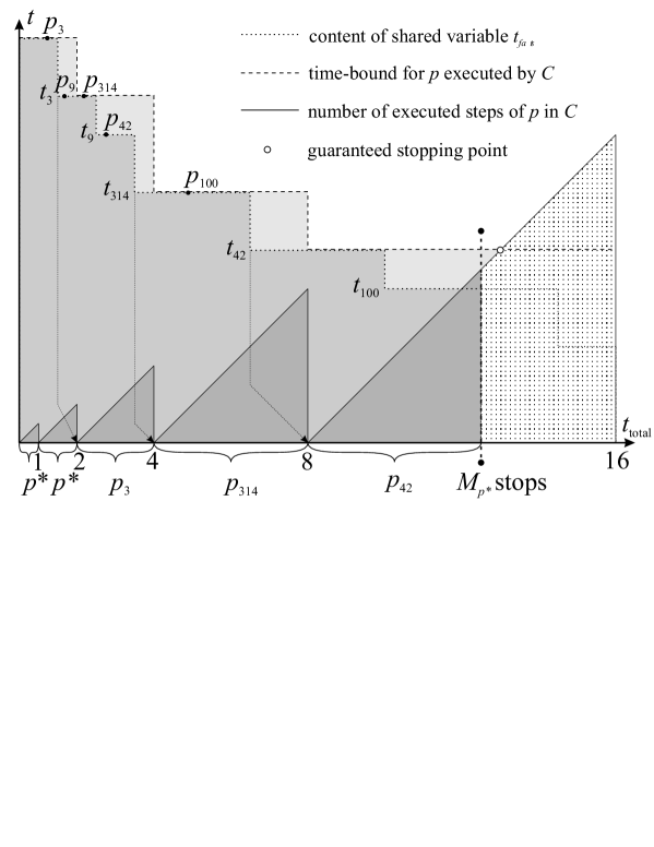
Figure 1: Sample execution of $M_{p^{*}}$. The horizontal axis marks the progress of $M_{p^{*}}$. The vertical axis marks general time-like quantities. The lower solid stepped curve is the content of variable $t_{fast}$ at time $t$. Black dots on this curve (denoted by $p$) mark events where algorithm $A$ creates and adds another valid program $p$ together with its time-bound $t$ to list $L$. The (later occurring) step in the curve marks the time when algorithm $B$ has computed $t(x)$ and updates $t_{fast}$. Algorithm $C$ starts $p$ at the next instruction step $k$ which is a power of 2 and executes $p$ for $k$ steps. This is illustrated by the exponentially increasing sawtooth curve. The time bound of $p$ during execution is indicated by the upper dashed stepped curve. Algorithm $M_{p^{*}}$ terminates when the stepped curve crosses the sawtooth curve (white circle), or earlier if the time-bound is not sharp.

5 Time Analysis

Henceforth we return to the convenient abbreviations $p(x)\!:=\!U(p,x)$ and $t_{p}(x)\!:=\!U(t_{p},x)$. Let $p^{\prime}$ be some fixed algorithm that is provably equivalent to $p^{*}$, with computation time $time_{p^{\prime}}$ provably bounded by $t_{p^{\prime}}$. Let ${l}(proof(p^{\prime}))$ be the length of the binary coding of the, for instance, shortest proof. Computation time always refers to true overall computation time, whereas computation steps refer to instruction steps. $steps=\alpha\!\cdot\!time$, if a percentage $\alpha$ of computation time is assigned to an algorithm.

A) To write down (not to invent!) a proof requires $O({l}(proof))$ steps. A time $O(N_{axiom}\!\cdot\!l(F_{i}))$ is needed to check whether a formula $F_{i}$ in the proof $F_{1}F_{2}...F_{n}$ is an axiom, where $N_{axiom}$ is the number of axioms or axiom-schemes, which is finite. Variable substitution (binding) can be performed in linear time. For a suitable set of axioms, the only necessary inference rule is modus ponens. If $F_{i}$ is not an axiom, one searches for a formula $F_{j}$, $j\!<\!i$ of the form $F_{k}\!\rightarrow\!F_{i}$ and then for the formula $F_{k}$, $k\!<\!i$. This takes time $O(l(proof))$. There are $n\leq O(l(proof))$ formulas $F_{i}$ to check in this way. Whether the sequence of formulas constitutes a valid proof can, hence, be checked in $O({l}(proof)^{2})$ steps. There are less than $2^{l+1}$ proofs of (binary) length $\leq\!l$. Algorithm $A$ receives $\alpha\!=\!10\%$ of relative computation time. Hence, for a proof of $(p^{\prime},t_{p^{\prime}})$ to occur, and for $(p^{\prime},t_{p^{\prime}})$ to be added to $L$, at most time $T_{A}\leq{1\over 10\%}\!\cdot\!2^{{l}(proof(p^{\prime}))+1}\!\cdot\!O({l}(proof(p^{\prime}))^{2})$ is needed. Note that the same program $p$ can and will be accompanied by different time bounds $t_{p}$; for instance $(p,time_{p})$ will occur.

B) The time assignment of algorithm $B$ to the $t_{p}$’s only works if the Kraft inequality $\sum_{(p,t_{p})\in L}2^{-{l}(p)-{l}(t_{p})}\leq 1$ is satisfied [10]. This can be ensured by using prefix free (e.g. Shannon-Fano) codes [17, 13]. The number of steps to calculate $t_{p^{\prime}}(x)$ is, by definition, $time_{t_{p^{\prime}}}(x)$. The relative computation time $\alpha$ available for computing $t_{p^{\prime}}(x)$ is $10\%\!\cdot\!2^{-{l}(p^{\prime})-{l}(t_{p^{\prime}})}$. Hence, $t_{p^{\prime}}(x)$ is computed and $t_{fast}\!\leq\!t_{p^{\prime}}(x)$ is checked after time $T_{B}\leq T_{A}+{1\over 10\%}\!\cdot\!2^{{l}(p^{\prime})+{l}(t_{p^{\prime}})}\!\cdot\!time_{t_{p^{\prime}}}(x)$. We have to add $T_{A}$, since $B$ has to wait, in the worst case, time $T_{A}$ before it can start executing $t_{p^{\prime}}(x)$.

C) If algorithm $C$ halts, its construction guarantees that the output is correct. In the following, we show that $C$ always halts, and give a bound for the computation time.

1. Assume that algorithm $C$ stops before $B$ performed the check $t_{p^{\prime}}(x)<t_{fast}$, because a different $p$ already computed $p(x)$. In this case $T_{C}\leq T_{B}$.

2. Assume that $k=k_{0}$ in $C$ when $B$ performs the check $t_{p^{\prime}}(x)<t_{fast}$. Running-time $T_{B}$ has passed until this point, hence $k_{0}\leq 80\%\!\cdot\!T_{B}$ . Furthermore, assume that $C$ halts in period $k_{0}$ because the program (different from $p^{\prime}$) executed in this period computes the result. In this case, $T_{C}\leq{1\over 80\%}2k_{0}\leq 2T_{B}$.

3. If $C$ does not halt in period $k_{0}$ but $2k_{0}\!\geq t_{fast}$, then $p^{\prime}(x)$ has enough time to compute the solution in the next period $k=2k_{0}$, since $time_{p^{\prime}}(x)\leq t_{fast}\leq 4k_{0}-2k_{0}$. Hence $T_{C}\leq{1\over 80\%}4k_{0}\leq 4T_{B}$.

4. Finally, if $2k_{0}\!<t_{fast}$ we “wait” for the period $k\!>\!k_{0}$ with ${\textstyle{1\over 2}}k\!\leq\!t_{fast}\!<\!k$. In this period $k$, either $p^{\prime}(x)$, or an even faster algorithm, which has in the meantime been constructed by A and B, will be computed. In any case, the $2k-k>t_{fast}$ steps are sufficient to compute the answer. We have ${80\%}\!\cdot\!T_{C}\leq 2k\leq 4t_{fast}\leq 4t_{p^{\prime}}(x)$.

The maximum of the cases (i) to (iv) bounds the computation time of $C$ and, hence, of $M_{p^{*}}$ by

$$time_{M_{p^{*}}}(x)=T_{C}\;\leq\;\max\{4T_{B},5t_{p}(x)\}\;\leq\;4T_{B}+5t_{p}(x)\;\leq\;$$

$$\;\leq\;5\!\cdot\!t_{p}(x)+d_{p}\!\cdot\!time_{t_{p}}(x)+c_{p}$$

$$d_{p}=40\!\cdot\!2^{{l}(p)+{l}(t_{p})},\quad c_{p}=40\!\cdot\!2^{{l}(proof(p))+1}\!\cdot\!O({l}(proof(p)^{2})$$

where we have dropped the prime from $p$. We have also suppressed the dependency of $c_{p}$ and $d_{p}$ on $p^{*}$ ($proof(p)$ depends on $p^{*}$ too), since we considered $p^{*}$ to be a fixed given algorithm. The factor of 5 may be reduced to $4+\varepsilon$ by assigning a larger fraction of time to algorithm $C$. The constants $c_{p}$ and $d_{p}$ will then be proportional to $1\over\varepsilon$. We were not able to further reduce this factor.

6 Assumptions on the Machine Model

In the time analysis above we have assumed that program simulation with abort possibility and scheduling parallel algorithms can be performed in real-time, i.e. without loss of performance. Parallel computation can be avoided by sequentially performing all operations for a limited time and then restarting all computations in a next cycle with double the time and so on. This will increase the computation time of $A$ and $B$ (but not of $C$!) by, at most, a factor of $4$. Note that we use the same universal Turing machine $U$ with the same underlying Turing machine model (number of heads, symbols, …) for measuring computation time of all programs (strings) $p$, including $M_{p^{*}}$. This prevents us from applying the linear speedup theorem (which is cheating somewhat anyway), but allows the possibility of designing a $U$ which allows real-time simulation with abort possibility. Small additive “patching” constants can be absorbed in the $O()$ notation of $c_{p}$. Theorem 1 should also hold for Kolmogorov-Uspenskii and Pointer machines.

7 Algorithmic Complexity and the Shortest Algorithm

Data compression is a very important issue in computer science. Saving space or channel capacity are obvious applications. A less obvious (but not far fetched) application is that of inductive inference in various forms (hypothesis testing, forecasting, classification, …). A free interpretation of Occam’s razor is that the shortest theory consistent with past data is the most likely to be correct. This has been put into a rigorous scheme by [18] and proved to be optimal in [19, 7]. Kolmogorov Complexity is a universal notion of the information content of a string [9, 4, 23]. It is defined as the length of the shortest program computing string $x$.

$$K_{U}(x)\;:=\;\min_{p}\{{l}(p):U(p)=x\}\;=\;K(x)+O(1)$$

where $U$ is some universal Turing Machine. It can be shown that $K_{U}(x)$ varies, at most, by an additive constant independent of $x$ by varying the machine $U$. Hence, the Kolmogorov Complexity $K(x)$ is universal in the sense that it is uniquely defined up to an additive constant. $K(x)$ can be approximated from above (is co-enumerable), but not finitely computable. See [13] for an excellent introduction to Kolmogorov Complexity and [22] for a review of Kolmogorov inspired prediction schemes.

Recently, Schmidhuber [15] has generalized Kolmogorov complexity in various ways to the limits of computability and beyond. In the following, we also need a generalization, but of a different kind. We need a short description of a function, rather than a string. The following definition of the complexity of a function $f$

$$K^{\prime}(f):=\min_{p}\{{l}(p):U(p,x)=f(x)\,\forall x\}$$

seems natural, but suffers from not even being approximable. There exists no algorithm converging to $K^{\prime}(f)$, because it is undecidable whether a program $p$ is the shortest program equivalent to a function $f$. Even if we have a program $p^{*}$ computing $f$, $K^{\prime}(p^{*})$ is not approximable. Using $K(p^{*})$ is not a suitable alternative, since $K(p^{*})$ might be considerably longer than $K^{\prime}(p^{*})$, as in the former case all information contained in $p^{*}$ will be kept – even that which is functionally irrelevant (e.g. dead code). An alternative is to restrict ourselves to provably equivalent programs. The length of the shortest one is

$$K^{\prime\prime}(p^{*})\;:=\;\min_{p}\{{l}(p):\mbox{a proof of }[\forall y\!:\!u(p,y)=u(p^{*},y)]\mbox{ exists}\}$$

It can be approximated from above, since the set of all programs provably equivalent to $p^{*}$ is enumerable.

Having obtained, after some time, a very short description $p^{\prime}$ of $p^{*}$ for some purpose (e.g. for defining a prior probability for some inductive inference scheme), it is usually also necessary to obtain values for some arguments. We are now concerned with the computation time of $p^{\prime}$. Could we get slower and slower algorithms by compressing $p^{*}$ more and more? Interestingly this is not the case. Inventing complex (long) programs is not necessary to construct asymptotically fast algorithms, under the stated provability assumptions, in contrast to Blum’s Theorem [2, 3]. The following theorem roughly says that there is a single program, which is the fastest and the shortest program.

Theorem 2. Let $p^{*}$ be a given algorithm or formal specification of a function. There exists a program $\tilde{p}$, equivalent to $p^{*}$, for which the following holds

$$\begin{array}[]{rl@{\;\leq\;}l}i)&{l}(\tilde{p})&K^{\prime\prime}(p^{*})+O(1)\\[4.30554pt] ii)&time_{\tilde{p}}(x)&5\!\cdot\!t_{p}(x)+d_{p}\!\cdot\!time_{t_{p}}(x)+c_{p}\end{array}$$

where $p$ is any program provably equivalent to $p^{*}$ with computation time provably less than $t_{p}(x)$. The constants $c_{p}$ and $d_{p}$ depend on $p$ but not on $x$.

To prove the theorem, we just insert the shortest algorithm $p^{\prime}$ provably equivalent to $p^{*}$ into $M$, that is $\tilde{p}:=M_{p^{\prime}}$. As only $O(1)$ instructions are needed to build $M_{p^{\prime}}$ from $p^{\prime}$, $M_{p^{\prime}}$ has size ${l}(p^{\prime})\!+\!O(1)=K^{\prime\prime}(p^{*})\!+\!O(1)$. The computation time of $M_{p^{\prime}}$ is the same as of $M_{p^{*}}$ apart from “slightly” different constants.

The following subtlety has been pointed out by Peter van Emde Boas. Neither $M_{p^{*}}$, nor $\tilde{p}$ is provably equivalent to $p^{*}$. The construction of $M_{p^{*}}$ in section 4 shows equivalence of $M_{p^{*}}$ (and of $\tilde{p}$) to $p^{*}$, but it is a meta-proof which cannot be formalized within the considered proof system. A formal proof of the correctness of $M_{p^{*}}$ would prove the consistency of the proof system, which is impossible by Gödels second incompleteness theorem. See [6] for details in a related context.

8 Generalizations

If $p^{*}$ has to be evaluated repeatedly, algorithm $A$ can be modified to remember its current state and continue operation for the next input ($A$ is independent of $x$!). The large offset time $c_{p}$ is only needed on the first invocation.

$M_{p^{*}}$ can be modified to handle i/o streams, definable by a Turing machine with monotone input and output tapes (and bidirectional working tapes) receiving an input stream and producing an output stream. The currently read prefix of the input stream is $x$. $time_{p}(x)$ is the time used for reading $x$. $M_{p^{*}}$ caches the input and output streams, so that algorithm $C$ can repeatedly read/write the streams for each new $p$. The true input/output tapes are used for requesting/producing a new symbol . Algorithm $B$ is reset after $1,2,4,8,...$ steps (not after reading the next symbol of $x$!) to appropriately take into account increased prefixes $x$. Algorithm $A$ just continues. The bound of Theorem 1 holds for this case too, with slightly increased $d_{p}$.

The construction above also works if time is measured in terms of the current output rather than the current input $x$. This measure is, for example, used for the time-complexity of calculating the $n^{th}$ digit of a computable real (e.g. $\pi$), where there is no input, but only an output stream.

9 Summary & Outlook

We presented an algorithm $M_{p^{*}}$ which accelerates the computation of a program $p^{*}$. $M_{p^{*}}$ combines ($A$) sequential search through proof space, ($B$) Levin search through time-bound space, ($C$) and sequential program execution, using a somewhat tricky scheduling. Under certain provability constraints, $M_{p^{*}}$ is the asymptotically fastest algorithm for computing $p^{*}$ apart from a factor 5 in computation time. Blum’s Theorem shows that the provability constraints are essential. We have shown that the conditions on Theorem 1 are often, but not always, satisfied for practical problems. For complex approximation problems, for instance, where no good and fast time bound exists, $M_{p^{*}}$ is still optimal, but in this case, only apart from a large multiplicative factor. We briefly outlined how $M_{p^{*}}$ can be modified to handle i/o streams and other time-measures. An interesting and counter-intuitive consequence of Theorem 1 was that the fastest program computing a certain function is also among the shortest programs provably computing this function. Looking for larger programs saves at most a finite number of computation steps, but cannot improve the time order. To quantify this statement, we extended the definition of Kolmogorov complexity and defined two novel natural measures for the complexity of a function. The large constants $c_{p}$ and $d_{p}$ seem to spoil a direct implementation of $M_{p^{*}}$. On the other hand, Levin search has been successfully applied to solve rather difficult machine learning problems [14, 16], even though it suffers from a large multiplicative factor of similar origin. The use of more elaborate theorem-provers, rather than brute force enumeration of all proofs, could lead to smaller constants and bring $M_{p}^{*}$ closer to practical applications, possibly restricted to subclasses of problems. A more fascinating (and more speculative) way may be the utilization of so called transparent or holographic proofs [1]. Under certain circumstances they allow an exponential speed up for checking proofs. This would reduce the constants $c_{p}$ and $d_{p}$ to their logarithm, which is a small value. I would like to conclude with a general question. Will the ultimate search for asymptotically fastest programs typically lead to fast or slow programs for arguments of practical size? Levin search, matrix multiplication and the algorithm $M_{p^{*}}$ seem to support the latter, but this might be due to our inability to do better.

Acknowledgements

Thanks to Monaldo Mastrolilli, Jürgen Schmidhuber, and Peter van Emde Boas for enlightening discussions and for useful comments. This work was supported by SNF grant 2000-61847.00.

References

- [1] L. Babai, L. Fortnow, L. A. Levin, and M. Szegedy. Checking computations in polylogarithmic time. STOC: 23rd ACM Symp. on Theory of Computation, 23:21–31, 1991.
- [2] M. Blum. A machine-independent theory of the complexity of recursive functions. Journal of the ACM, 14(2):322–336, 1967.
- [3] M. Blum. On effective procedures for speeding up algorithms. Journal of the ACM, 18(2):290–305, 1971.
- [4] G. J. Chaitin. On the length of programs for computing finite binary sequences. Journal of the ACM, 13(4):547–569, 1966.
- [5] Melvin C. Fitting. First-Order Logic and Automated Theorem Proving. Graduate Texts in Computer Science. Springer-Verlag, Berlin, 2nd edition, 1996.
- [6] J. Hartmanis. Relations between diagonalization, proof systems, and complexity gaps. Theoretical Computer Science, 8(2):239–253, April 1979.
- [7] M. Hutter. New error bounds for Solomonoff prediction. Journal of Computer and System Science, in press, 1999. ftp://ftp.idsia.ch/pub/techrep/IDSIA-11-00.ps.gz.
- [8] M. Hutter. A theory of universal artificial intelligence based on algorithmic complexity. Technical report, 62 pages, 2000. http://arxiv.org/abs/cs.AI/0004001.
- [9] A. N. Kolmogorov. Three approaches to the quantitative definition of information. Problems of Information and Transmission, 1(1):1–7, 1965.
- [10] L. G. Kraft. A device for quantizing, grouping and coding amplitude modified pulses. Master’s thesis, Cambridge, MA, 1949.
- [11] L. A. Levin. Universal sequential search problems. Problems of Information Transmission, 9:265–266, 1973.
- [12] L. A. Levin. Randomness conservation inequalities: Information and independence in mathematical theories. Information and Control, 61:15–37, 1984.
- [13] M. Li and P. M. B. Vitányi. An introduction to Kolmogorov complexity and its applications. Springer, 2nd edition, 1997.
- [14] J. Schmidhuber. Discovering neural nets with low Kolmogorov complexity and high generalization capability. Neural Networks, 10(5):857–873, 1997.
- [15] J. Schmidhuber. Algorithmic theories of everything. Report IDSIA-20-00, quant-ph/0011122, IDSIA, Manno (Lugano), Switzerland, 2000.
- [16] J. Schmidhuber, J. Zhao, and M. Wiering. Shifting inductive bias with success-story algorithm, adaptive Levin search, and incremental self-improvement. Machine Learning, 28:105–130, 1997.
- [17] C. E. Shannon. A mathematical theory of communication. Bell System Technical Journal, 27:379–423, 623–656, 1948. Shannon-Fano codes.
- [18] R. J. Solomonoff. A formal theory of inductive inference: Part 1 and 2. Inform. Control, 7:1–22, 224–254, 1964.
- [19] R. J. Solomonoff. Complexity-based induction systems: comparisons and convergence theorems. IEEE Trans. Inform. Theory, IT-24:422–432, 1978.
- [20] R. J. Solomonoff. Applications of algorithmic probability to artificial intelligence. In Uncertainty in Artificial Intelligence, pages 473–491. Elsevier Science Publishers, 1986.
- [21] V. Strassen. Gaussian elimination is not optimal. Numerische Mathematik, 13:354–356, 1969.
- [22] P. M. B. Vitányi and M. Li. Minimum description length induction, Bayesianism, and Kolmogorov complexity. IEEE Transactions on Information Theory, 46(2):446–464, 2000.
- [23] A. K. Zvonkin and L. A. Levin. The complexity of finite objects and the development of the concepts of information and randomness by means of the theory of algorithms. RMS: Russian Mathematical Surveys, 25(6):83–124, 1970.