A Statistical Physics Perspective on Web Growth

Abstract

Approaches from statistical physics are applied to investigate the structure of network models whose growth rules mimic aspects of the evolution of the world-wide web. We first determine the degree distribution of a growing network in which nodes are introduced one at a time and attach to an earlier node of degree $k$ with rate $A_{k}\sim k^{\gamma}$. Very different behaviors arise for $\gamma<1$, $\gamma=1$, and $\gamma>1$. We also analyze the degree distribution of a heterogeneous network, the joint age-degree distribution, the correlation between degrees of neighboring nodes, as well as global network properties. An extension to directed networks is then presented. By tuning model parameters to reasonable values, we obtain distinct power-law forms for the in-degree and out-degree distributions with exponents that are in good agreement with current data for the web. Finally, a general growth process with independent introduction of nodes and links is investigated. This leads to independently growing sub-networks that may coalesce with other sub-networks. General results for both the size distribution of sub-networks and the degree distribution are obtained.

1 Introduction

With the recent appearance of the Internet and the world-wide web, understanding the properties of growing networks with popularity-based construction rules has become an active and fruitful research area [1]. In such models, newly-introduced nodes preferentially attach to pre-existing nodes of the network that are already “popular”. This leads to graphs whose structure is quite different from the well-known random graph [2, 3] in which links are created at random between nodes without regard to their popularity. This discovery of a new class of graph theory problems has fueled much effort to characterize their properties.

One basic measure of the structure of such networks is the node degree $N_{k}$ defined as the number of nodes in the network that are linked to $k$ other nodes. In the case of the random graph, the node degree is simply a Poisson distribution. In contrast, many popularity-driven growing networks have much broader degree distributions with a stretched exponential or a power-law tail. The latter form means that there is no characteristic scale for the node degree, a feature that typifies many networked systems [1].

Power laws, or more generally, distributions with highly skewed tails, characterize the degree distributions of many man-made and naturally occurring networks [1]. For example, the degree distributions at the level of autonomous systems and at the router level exhibit highly skewed tails [4, 5, 6]. Other important Internet-based graphs, such as the hyperlink graph of the world-wide web also appear to have a degree distribution with a power-law tail [7, 8, 9, 10, 11]. These observations have spurred a flurry of recent work to understand the underlying mechanisms for these phenomena.

A related example with interest to anyone who publishes, is the distribution of scientific citations [12, 13, 14]. Here one treats publications as nodes and citations as links in a citation graph. Currently-available data suggests that the citation distribution has a power-law tail with an associated exponent close to $-3$ [14]. As we shall see, this exponent emerges naturally in the Growing Network (GN) model where the relative probability of linking from a new node to a previous node (equivalent to citing an earlier paper) is strictly proportional to the popularity of the target node.

In this paper, we apply tools from statistical physics, especially the rate equation approach, to quantify the structure of growing networks and to elucidate the types of geometrical features that arise in networks with physically-motivated growth rules. The utility of the rate equations has been demonstrated in a diverse range of phenomena in non-equilibrium statistical physics, such as aggregation [15], coarsening [16], and epitaxial surface growth [17]. We will attempt to convince the reader that the rate equations are also a simple yet powerful analysis tool to analyze growing network systems. In addition to providing comprehensive information about the node degree distribution, the rate equations can be easily adapted to analyze both heterogeneous and directed networks, the age distribution of nodes, correlations between node degrees, various global network properties, as well as the cluster size distribution in models that give rise to independently evolving sub-networks. Thus the rate equation method appears to be better suited for probing the structure of growing networks compared to the classical approaches for analyzing random graphs, such as probabilistic [2] or generating function [3] techniques.

In the next section, we introduce three basic models that will be the focus of this review. In the following three sections, we then present rate equation analyses to determine basic geometrical properties of these networks. We close with a brief summary.

2 Models

The models we study appear to embody many of the basic growth processes in web graphs and related systems. These include:

• The Growing Network (GN) [8, 18]. Nodes are added one at a time and a single link is established between the new node and a pre-existing node according to an attachment probability $A_{k}$ that depends only on the degree of the “target” node (Fig. 1).

  

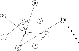
  Figure 1: Growing network. Nodes are added sequentially and a single link joins a new node to an earlier node. Node 1 has (total) degree 5, node 2 has degree 3, nodes 4 and 6 have degree 2, and the remaining nodes have degree 1.

• The Web Graph (WG). This represents an extension of the GN to incorporate link directionality [19] and leads to independent, dynamically generated in-degree and out-degree distributions. The network growth occurs by two distinct processes [20] that are meant to mimic how hyperlinks are created in the web (Fig. 2):

  • With probability $p$, a new node is introduced and it immediately attaches to an earlier target node. The attachment probability depends only on the in-degree of the target.

  • With probability $q=1-p$, a new link is created between already existing nodes. The choices of the originating and target nodes depend on the out-degree of the former and the in-degree of the latter.

  

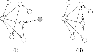
  Figure 2: Growth processes in the web graph model: (i) node creation and immediate attachment, and (ii) link creation. In (i) the new node is shaded, while in both (i) and (ii) the new link is dashed.

• The Multicomponent Graph (MG). Nodes and links are introduced independently [21]. (i) With probability $p$, a new unlinked node is introduced, while (ii) with probability $q=1-p$, a new link is created between existing nodes. As in the WG, the choices of the originating and target nodes depend on the out-degree of the former and the in-degree of the latter. Step (i) allows for the formation of many clusters.

3 Structure of the Growing Network

Because of its simplicity, we first study the structure of the GN [8, 18]. The basic approaches developed in this section will then be extended to the WG and MG models.

3.1 Degree Distribution of a Homogeneous Network

We first focus on the node degree distribution $N_{k}$. To determine its evolution, we shall write the rate equations that account for the change in the degree distribution after each node addition event. These equations contain complete information about the node degree, from which any measure of node degree (such as moments) can be easily extracted. For the GN growth process in which nodes are introduced one at a time, the rate equations for the degree distribution $N_{k}(t)$ are [22]

$${dN_{k}\over dt}={A_{k-1}N_{k-1}-A_{k}N_{k}\over A}+\delta_{k1}.$$ (3.1)

The first term on the right, $A_{k-1}N_{k-1}/A$, accounts for processes in which a node with $k-1$ links is connected to the new node, thus increasing $N_{k}$ by one. Since there are $N_{k-1}$ nodes of degree $k-1$, the rate at which such processes occur is proportional to $A_{k-1}N_{k-1}$, and the factor $A(t)=\sum_{j\geq 1}A_{j}N_{j}(t)$ converts this rate into a normalized probability. A corresponding role is played by the second (loss) term on the right-hand side; $A_{k}N_{k}/A$ is the probability that a node with $k$ links is connected to the new node, thus leading to a loss in $N_{k}$. The last term accounts for the introduction of new nodes with no incoming links.

We start by solving for the time dependence of the moments of the degree distribution defined via $M_{n}(t)=\sum_{j\geq 1}j^{n}N_{j}(t)$. This is a standard method of analysis of rate equations by which one can gain partial, but valuable, information about the time dependence of the system with minimal effort. By explicitly summing Eqs. (3.1) over all $k$, we easily obtain $\dot{M}_{0}(t)=1$, whose solution is $M_{0}(t)=M_{0}(0)+t$. Notice that by definition $M_{0}(t)=\sum_{k}N_{k}$ is just the total number of nodes in the network. It is clear by the nature of the growth process that this quantity simply grows as $t$. In a similar fashion, the first moment of the degree distribution obeys $\dot{M}_{1}(t)=2$ with solution $M_{1}(t)=M_{1}(0)+2t$. This time evolution for $M_{1}$ can be understood either by explicitly summing the rate equations, or by observing that this first moment simply equals the total number of link endpoints. Clearly, this quantity must grow as $2t$ since the introduction of a single node introduces two link endpoints. Thus we find the simple result that the first two moments are independent of the attachment kernel $A_{k}$ and grow linearly with time. On the other hand, higher moments and the degree distribution itself do depend in an essential way on the kernel $A_{k}$.

As a preview to the general behavior for the degree distribution, consider the strictly linear kernel [8, 22, 23], for which $A(t)$ coincides with $M_{1}(t)$. In this case, we can solve Eqs. (3.1) for an arbitrary initial condition. However, since the long-time behavior is most interesting, we limit ourselves to the asymptotic regime ($t\to\infty$) where the initial condition is irrelevant. Using therefore $M_{1}=2t$, we solve the first few of Eqs. (3.1) directly and obtain $N_{1}=2t/3$, $N_{2}=t/6$, etc. Thus each of the $N_{k}$ grow linearly with time. Accordingly, we substitute $N_{k}(t)=t\,n_{k}$ in Eqs. (3.1) to yield the simple recursion relation $n_{k}=n_{k-1}(k-1)/(k+2)$. Solving for $n_{k}$ gives

$$n_{k}={4\over k(k+1)(k+2)}.$$ (3.2)

Returning to the case of general attachment kernels, let us assume that the degree distribution and $A(t)$ both grow linearly with time. This hypothesis can be easily verified numerically for attachment kernels that do not grow faster than linearly with $k$. Then substituting $N_{k}(t)=t\,n_{k}$ and $A(t)=\mu t$ into Eqs. (3.1) we obtain the recursion relation $n_{k}=n_{k-1}A_{k-1}/(\mu+A_{k})$ and $n_{1}=\mu/(\mu+A_{1})$. Finally, solving for $n_{k}$, we obtain the formal expression

$$n_{k}={\mu\over A_{k}}\prod_{j=1}^{k}\left(1+{\mu\over A_{j}}\right)^{-1}.$$ (3.3)

To complete the solution, we need the amplitude $\mu$. Using the definition $\mu=\sum_{j\geq 1}A_{j}n_{j}$ in Eq. (3.3), we obtain the implicit relation

$$\sum_{k=1}^{\infty}\prod_{j=1}^{k}\left(1+{\mu\over A_{j}}\right)^{-1}=1$$ (3.4)

which shows that the amplitude $\mu$ depends on the entire attachment kernel.

For the generic case $A_{k}\sim k^{\gamma}$, we substitute this form into Eq. (3.3) and then rewrite the product as the exponential of a sum of a logarithm. In the continuum limit, we convert this sum to an integral, expand the logarithm to lowest order, and then evaluate the integral to yield the following basic results:

$$n_{k}\sim\cases{k^{-\gamma}\exp\left[-\mu\left({{k^{1-\gamma}-2^{1-\gamma}}\over 1-\gamma}\right)\right],&$0\leq\gamma<1$;\cr k^{-\nu},\quad\nu>2,&$\gamma=1$;\cr{\rm best\ seller}&$1<\gamma<2$;\cr{\rm bible}&$2<\gamma$.}$$ (3.5)

Thus the degree distribution decays exponentially for $\gamma=0$, as in the case of the random graph, while for all $0<\gamma<1$, the distribution exhibits robust stretched exponential behavior. The linear kernel is the case that has garnered much of the current research interest. As shown above, $n_{k}={4/[k(k+1)(k+2)]}$ for the strictly linear kernel $A_{k}=k$. One might anticipate that $n_{k}\propto k^{-3}$ holds for all asymptotically linear kernels, $A_{k}\sim k$. However, the situation is more delicate and the degree distribution exponent depends on microscopic details of $A_{k}$. From Eq. (3.3), we obtain $n_{k}\sim k^{-\nu}$, where the exponent $\nu=1+\mu$ can be tuned to any value larger than 2 [22, 24]. This non-universal behavior shows that one must be cautious in drawing general conclusions from the GN with a linear attachment kernel.

Figure 3: A node with in-degree $i=4$, out-degree $j=5$, and total degree 9.

As an illustrative example of the vagaries of asymptotically linear kernels, consider the shifted linear kernel $A_{k}=k+w$. One way to motivate this kernel is to explicitly keep track of link directionality. In particular, the node degree for an undirected graph naturally generalizes to the in-degree and out-degree for a directed graph, the number of incoming and outgoing links at a node, respectively. Thus the total degree $k$ in a directed graph is the sum of the in-degree $i$ and out-degree $j$ (Fig. 3). (More details on this model are given in the next section.)  The most general linear attachment kernel for a directed graph has the form $A_{ij}=ai+bj$. The GN corresponds to the case where the out-degree of any node equals one; thus $j=1$ and $k=i+1$. For this example the general linear attachment kernel reduces to $A_{k}=a(k-1)+b$. Since the overall scale is irrelevant, we can re-write $A_{k}$ as the shifted linear kernel $A_{k}=k+w$, with $w=-1+b/a$ that can vary over the range $-1<w<\infty$.

To determine the degree distribution for the shifted linear kernel, note that $A(t)=\sum_{j}A_{j}N_{j}(t)$ simply equals $A(t)=M_{1}(t)+wM_{0}(t)$. Using $A=\mu t$, $M_{0}=t$ and $M_{1}=2t$, we get $\mu=2+w$ and hence the relation $\nu=1+\mu$ from the previous paragraph becomes $\nu=3+w$. Thus a simple additive shift in the attachment kernel profoundly affects the asymptotic degree distribution. Furthermore, from Eq. (3.3) we determine the entire degree distribution to be

$$n_{k}=(2+w)\,{\Gamma(3+2w)\over\Gamma(1+w)}\,{\Gamma(k+w)\over\Gamma(k+3+2w)}.$$ (3.6)

Finally, we outline the intriguing behavior for super-linear kernels. In this case, there is a “runaway” or gelation-like phenomenon in which one node links to almost every other node. For $\gamma>2$, all but a finite number of nodes are linked to a single node that has the rest of the links. We term such an overwhelmingly popular node as a “bible”. For $1<\gamma\leq 2$, the number of nodes with a just a few links is no longer finite, but grows slower than linearly in time, and the remainder of the nodes are linked to an extremely popular node that we now term “best seller”. Full details about this runaway behavior are given in [22].

As a final parenthetical note, when the attachment kernel has the form $A_{k}\propto k^{\gamma}$, with $\gamma<0$, there is preferential attachment to poorly-connected sites. Here, the degree distribution exhibits faster than exponential decay, $n_{k}\propto k^{-\gamma(k-1)}$. When $\gamma<-2$, the propensity for avoiding popularity is so strong that there is a finite probability of forming a “worm” graph in which each node attaches only to its immediate predecessor.

3.2 Degree Distribution of a Heterogeneous Network

A practically-relevant generalization of the GN is to endow each node with an intrinsic and permanently defined “attractiveness” [25]. This accounts for the obvious fact that not all nodes are equivalent, but that some are clearly more attractive than others at their inception. Thus the subsequent attachment rate to a node should be a function of both its degree and its intrinsic attractiveness. For this generalization, the rate equation approach yields complete results with minimal additional effort beyond that needed to solve the homogeneous network.

Let us assign each node an attractiveness parameter $\eta>0$, with arbitrary distribution, at its inception. This attractiveness modifies the node attachment rate as follows: for a node with degree $k$ and attractiveness $\eta$, the attachment rate is simply $A_{k}(\eta)$. Now we need to characterize nodes both by their degree and their attractiveness – thus $N_{k}(\eta)$ is the number of nodes with degree $k$ and attractiveness $\eta$. This joint degree-attractiveness distribution obeys the rate equation,

$${dN_{k}(\eta)\over dt}={A_{k-1}(\eta)N_{k-1}(\eta)-A_{k}(\eta)N_{k}(\eta)\over A}+p_{0}(\eta)\delta_{k1}.$$ (3.7)

Here $p_{0}(\eta)$ is the probability that a newly-introduced node has attractiveness $\eta$, and the normalization factor $A=\int d\eta\sum_{k}A_{k}(\eta)N_{k}(\eta)$.

Following the same approach as that used to analyze Eq. (3.1), we substitute $A=\mu t$ and $n_{k}(\eta)=tN_{k}(\eta)$ into Eq. (3.7) to obtain the recursion relation

$$n_{k}(\eta)=p_{0}(\eta){\mu\over A_{k}(\eta)}\prod_{j=1}^{k}\left(1+{\mu\over A_{j}(\eta)}\right)^{-1}.$$ (3.8)

For concreteness, consider the linear attachment kernel $A_{k}(\eta)=\eta k$. Then applying the same analysis as in the homogeneous network, we find

$$n_{k}(\eta)={\mu\,p_{0}(\eta)\over\eta}\,{\Gamma(k)\,\Gamma\left(1+{\mu\over\eta}\right)\over\Gamma\left(k+1+{\mu\over\eta}\right)}.$$ (3.9)

To determine the amplitude $\mu$ we substitute (3.9) into the definition $\mu=\int d\eta\,\sum_{k\geq 1}A_{k}(\eta)\,n_{k}(\eta)$ and use the identity [26]

$$\sum_{k=1}^{\infty}{\Gamma(k+u)\over\Gamma(k+v)}={\Gamma(u+1)\over(v-u-1)\,\Gamma(v)}$$

to simplify the sum. This yields the implicit relation

$$1=\int d\eta\,p_{0}(\eta)\,\left({\mu\over\eta}-1\right)^{-1}.$$ (3.10)

This condition on $\mu$ leads to two alternatives: If the support of $\eta$ is unbounded, then the integral diverges and there is no solution for $\mu$. In this limit, the most attractive node is connected to a finite fraction of all links. Conversely, if the support of $\eta$ is bounded, the resulting degree distribution is similar to that of the homogeneous network. For fixed $\eta$, $n_{k}(\eta)\sim k^{-\nu(\eta)}$ with an attractiveness-dependent decay exponent $\nu(\eta)=1+\mu/\eta$. Amusingly, the total degree distribution $n_{k}=\int d\eta\,n_{k}(\eta)$ is no longer a strict power law [25]. Rather, the asymptotic behavior is governed by properties of the initial attractiveness distribution near the upper cutoff. In particular, if $p_{0}(\eta)\sim(\eta_{\rm max}-\eta)^{\omega-1}$ (with $\omega>0$ to ensure normalization), the total degree distribution exhibits a logarithmic correction

$$n_{k}\sim k^{-(1+\mu/\eta_{\rm max})}\,(\ln k)^{-\omega}.$$ (3.11)

3.3 Age Distribution

In addition to the degree distribution, we determine when connections occur. Naively, we expect that older nodes will be better connected. We study this feature by resolving each node both by its degree and its age to provide a more complete understanding of the network evolution. Thus define $c_{k}(t,a)$ to be the average number of nodes of age $a$ that have $k-1$ incoming links at time $t$. Here age $a$ means that the node was introduced at time $t-a$. The original degree distribution may be recovered from the joint age-degree distribution through $N_{k}(t)=\int_{0}^{t}da\,c_{k}(t,a)$.

For simplicity, we consider only the case of the strictly linear kernel; more general kernels were considered in Ref. [24]. The joint age-degree distribution evolves according to the rate equation

$$\left({\partial\over\partial t}+{\partial\over\partial a}\right)c_{k}={A_{k-1}c_{k-1}-A_{k}c_{k}\over 2t}+\delta_{k1}\delta(a).$$ (3.12)

The second term on the left accounts for the aging of nodes. We assume here that the probability of linking to a given node again depends only on its degree and not on its age. Finally, we again have used $A(t)\equiv M_{1}(t)\simeq 2t$ for the linear attachment kernel in the long-time limit.

The homogeneous form of this equation implies that solution should be self-similar. Thus we seek a solution as a function of the single variable $a/t$ rather than two separate variables. Writing $c_{k}(t,a)=f_{k}(x)$ with $x=1-{a\over t}$, we convert Eq. (3.12) into the ordinary differential equation

$$-2x\,{df_{k}\over dx}=(k-1)f_{k-1}-kf_{k}.$$ (3.13)

We omit the delta function term, since it merely provides the boundary condition $c_{k}(t,a=0)=\delta_{k1}$, or $f_{k}(1)=\delta_{k1}$.

The solution to this boundary-value problem may be simplified by assuming the exponential solution $f_{k}=\Phi\varphi^{k-1}$; this is consistent with the boundary condition, provided that $\Phi(1)=1$ and $\varphi(1)=0$. This ansatz reduces the infinite set of rate equations (3.13) into two elementary differential equations for $\varphi(x)$ and $\Phi(x)$ whose solutions are $\varphi(x)=1-\sqrt{x}$ and $\Phi(x)=\sqrt{x}$. In terms of the original variables of $a$ and $t$, the joint age-degree distribution is then

$$c_{k}(t,a)=\sqrt{1-{a\over t}}\left\{1-\sqrt{1-{a\over t}}\right\}^{k-1}.$$ (3.14)

Thus the degree distribution for fixed-age nodes decays exponentially, with a characteristic degree that diverges as $\langle k\rangle\sim(1-a/t)^{-1/2}$ for $a\to t$. As expected, young nodes (those with $a/t\to 0$) typically have a small degree while old nodes have large degree (Fig. 4). It is the large characteristic degree of old nodes that ultimately leads to a power-law total degree distribution when the joint age-degree distribution is integrated over all ages.

Figure 4: Age-dependent degree distribution for the GN for the linear attachment kernel. Low-degree nodes tend to be relatively young while high-degree nodes are old. The inset shows detail for $a/t\geq 0.98$.

3.4 Node Degree Correlations

The rate equation approach is sufficiently versatile that we can also obtain much deeper geometrical properties of growing networks. One such property is the correlation between degrees of connected nodes [24]. These develop naturally because a node with large degree is likely to be old. Thus its ancestor is also old and hence also has a large degree. In the context of the web, this correlation merely expresses that obvious fact that it is more likely that popular web sites have hyperlinks among each other rather than to marginal sites.

To quantify the node degree correlation, we define $C_{kl}(t)$ as the number of nodes of degree $k$ that attach to an ancestor node of degree $l$ (Fig. 5). For example, in the network of Fig. 1, there are $N_{1}=6$ nodes of degree 1, with $C_{12}=C_{13}=C_{15}=2$. There are also $N_{2}=2$ nodes of degree 2, with $C_{25}=2$, and $N_{3}=1$ nodes of degree 3, with $C_{35}=1$.

Figure 5: Definition of the node degree correlation $C_{kl}$ for the case $k=3$ and $l=4$.

For simplicity, we again specialize to the case of the strictly linear attachment kernel. More general kernels can also be treated within our general framework [24]. For the linear attachment kernel, the degree correlation $C_{kl}(t)$ evolves according to the rate equation

$$M_{1}\,{dC_{kl}\over dt}=(k-1)C_{k-1,l}-kC_{kl}+(l-1)C_{k,l-1}-lC_{kl}+(l-1)C_{l-1}\,\delta_{k1}.$$ (3.15)

The processes that gives rise to each term in this equation are illustrated in Fig. 6. The first two terms on the right account for the change in $C_{kl}$ due to the addition of a link onto a node of degree $k-1$ (gain) or $k$ (loss) respectively, while the second set of terms gives the change in $C_{kl}$ due to the addition of a link onto the ancestor node. Finally, the last term accounts for the gain in $C_{1l}$ due to the addition of a new node.

Figure 6: The processes that contribute ((i)–(v) in order) to the various terms in the rate equation (3.15). The newly-added node and link are shown dashed.

As in the case of the node degree, the time dependence can be separated as $C_{kl}=tc_{kl}$. This reduces Eqs. (3.15) to the time-independent recursion relation,

$$(k+l+2)c_{kl}=(k-1)c_{k-1,l}+(l-1)c_{k,l-1}+(l-1)c_{l-1}\,\delta_{k1}.$$ (3.16)

This can be further reduced to a constant-coefficient inhomogeneous recursion relation by the substitution

$$c_{kl}={\Gamma(k)\,\Gamma(l)\over\Gamma(k+l+3)}\,\,d_{kl}$$

to yield

$$d_{kl}=d_{k-1,l}+d_{k,l-1}+4(l+2)\delta_{k1}.$$ (3.17)

Solving Eqs. (3.17) for the first few $k$ yields the pattern of dependence on $k$ and $l$ from which one can then infer the solution

$$d_{kl}=4\,{\Gamma(k+l)\over\Gamma(k+2)\,\Gamma(l-1)}+12\,{\Gamma(k+l-1)\over\Gamma(k+1)\,\Gamma(l-1)},$$ (3.18)

from which we ultimately obtain

$$c_{kl}={4(l-1)\over k(k+l)(k+l+1)(k+l+2)}\left[{1\over k+1}+{3\over k+l-1}\right].$$ (3.19)

The important feature of this result is that the joint distribution does not factorize, that is, $c_{kl}\neq n_{k}n_{l}$. This correlation between the degrees of connected nodes is an important distinction between the GN and classical random graphs.

While the solution of Eq. (3.19) is unwieldy, it greatly simplifies in the scaling regime, $k\to\infty$ and $l\to\infty$ with $y=l/k$ finite. The scaled form of the solution is

$$c_{kl}=k^{-4}\,{4y(y+4)\over(1+y)^{4}}.$$ (3.20)

For fixed large $k$, the distribution $c_{kl}$ has a single maximum at $y^{*}=(\sqrt{33}-5)/2\cong 0.372$. Thus a node whose degree $k$ is large is typically linked to another node whose degree is also large; the typical degree of the ancestor is 37% that of the daughter node. In general, when $k$ and $l$ are both large and their ratio is different from one, the limiting behaviors of $c_{kl}$ are

$$c_{kl}\to\cases{16\,(l/k^{5})&$l\ll k$,\cr 4/(k^{2}\,l^{2})&$l\gg k$.\cr}$$ (3.21)

Here we explicitly see the absence of factorization in the degree correlation: $c_{kl}\neq n_{k}n_{l}\propto(k\,l)^{-3}$.

3.5 Global Properties

In addition to elucidating the degree distribution and degree correlations, the rate equations can be applied to determine global properties. One useful example is the out-component with respect to a given node x – this is the set of nodes that can be reached by following directed links that emanate from x (Fig. 7). In the context of the web, this is the set of nodes that are reached by following hyperlinks that emanate from a fixed node to target nodes, and then iteratively following target nodes ad infinitum. In a similar vein, one may enumerate all nodes that refer to a fixed node, plus all nodes that refer these daughter nodes, etc. This progeny comprises the in-component to node x – the set from which x can be reached by following a path of directed links.

Figure 7: In-component and out-components of node x.

3.5.1 The In-Component

For simplicity, we study the in-component size distribution for the GN with a constant attachment kernel, $A_{k}=1$. We consider this kernel because many results about network components are independent of the form of the kernel and thus it suffices to consider the simplest situation; the extension to more general attachment kernels is discussed in [24].

For the constant attachment kernel, the number $I_{s}(t)$ of in-components with $s$ nodes satisfies the rate equation

$${dI_{s}\over dt}={(s-1)I_{s-1}-sI_{s}\over A}+\delta_{s1}.$$ (3.22)

The loss term accounts for processes in which the attachment of a new node to an in-component of size $s$ increases its size by one. This gives a loss rate that is proportional to $s$. If there is more than one in-component of size $s$ they must be disjoint, so that the total loss rate for $I_{s}(t)$ is simply $sI_{s}(t)$. A similar argument applies for the gain term. Finally, dividing by $A(t)=\sum_{j}A_{j}N_{j}(t)$ converts these rates to normalized probabilities. For the constant attachment kernel, $A(t)=M_{0}(t)$, so asymptotically $A=t$. Interestingly, Eq. (3.22) is almost identical to the rate equations for the degree distribution for the GN with linear attachment kernel, except that the prefactor equals $t^{-1}$ rather than $(2t)^{-1}$. This change in the normalization factor is responsible for shifting the exponent of the resulting distribution from $-3$ to $-2$.

To determine $I_{s}(t)$, we again note, by explicitly solving the first few of the rate equations, that each $I_{s}$ grows linearly in time. Thus we substitute $I_{s}(t)=ti_{s}$ into Eqs. (3.22) to obtain $i_{1}=1/2$ and $i_{s}=i_{s-1}(s-1)/(s+1)$. This immediately gives

$$i_{s}={1\over s(s+1)}.$$ (3.23)

This $s^{-2}$ tail for the in-component distribution is a robust feature, independent of the form of the attachment kernel [24]. This $s^{-2}$ tail also agrees with recent measurements of the web [10].

3.5.2 The Out-Component

The complementary out-component from each node can be determined by constructing a mapping between the out-component and an underlying network “genealogy”. We build a genealogical tree for the GN by taking generation $g=0$ to be the initial node. Nodes that attach to those in generation $g$ form generation $g+1$; the node index does not matter in this characterization. For example, in the network of Fig. 1, node 1 is the “ancestor” of 6, while 10 is the “descendant” of 6 and there are 5 nodes in generation $g=1$ and 4 in $g=2$. This leads to the genealogical tree of Fig. 8.

Figure 8: Genealogy of the network in Fig. 1. The nodes indices indicate when each is introduced. The nodes are also arranged according to generation number.

The genealogical tree provides a convenient way to characterize the out-component distribution. As one can directly verify from Fig. 8, the number $O_{s}$ of out-components with $s$ nodes equals $L_{s-1}$, the number of nodes in generation $s-1$ in the genealogical tree. We therefore compute $L_{g}(t)$, the size of generation $g$ at time $t$. For this discussion, we again treat only the constant attachment kernel and refer the reader to Ref. [24] for more general attachment kernels. We determine $L_{g}(t)$ by noting that $L_{g}(t)$ increases when a new node attaches to a node in generation $g-1$. This occurs with rate $L_{g-1}/M_{0}$, where $M_{0}(t)=1+t$ is the number of nodes. This gives the differential equation for $\dot{L}_{g}(t)=L_{g-1}/(1+t)$ with solution $L_{g}(\tau)={\tau^{g}/g!}$, where $\tau=\ln(1+t)$. Thus the number $O_{s}$ of out-components with $s$ nodes equals

$$O_{s}(\tau)={\tau^{s-1}/(s-1)!}.$$ (3.24)

Note that the generation size $L_{g}(t)$ grows with $g$, when $g<\tau$, and then decreases and becomes of order 1 when $g=e\tau$. The genealogical tree therefore contains approximately $e\tau$ generations at time $t$. This result allows us to determine the diameter of the network, since the maximum distance between any pair of nodes is twice the distance from the root to the last generation. Therefore the diameter of the network scales as $2e\tau\approx 2e\ln N$; this is the same dependence on $N$ as in the random graph [2, 3]. More importantly, this result shows that the diameter of the GN is always small – ranging from the order of $\ln N$ for a constant attachment kernel, to the order of one for super-linear attachment kernels.

4 The Web Graph

In the world-wide web, link directionality is clearly relevant, as hyperlinks go from an issuing website to a target website but not vice versa. Thus to characterize the local graph structure more fully, the node degree should be resolved into the in-degree – the number of incoming links to a node, and the complementary out-degree (Fig. 3). Measurements on the web indicate that these distributions are power laws with different exponents [11]. These properties can be accounted for by the web graph (WG) model (Fig. 2) and the rate equations provide an extremely convenient analysis tool.

4.1 Average Degrees

Let us first determine the average node degrees (in-degree, out-degree, and total degree) of the WG. Let $N(t)$ be the total number of nodes, and $I(t)$ and $J(t)$ the in-degree and out-degree of the entire network, respectively. According to the elemental growth steps of the model, these degrees evolve by one of the following two possibilities:

$$(N,I,J)\to\cases{(N+1,I+1,J+1)&with probability $p$,\cr(N,I+1,J+1)&with probability $q$.}$$

That is, with probability $p$ a new node and new directed link are created (Fig. 2) so that the number of nodes and both the total in- and out-degrees increase by one. Conversely, with probability $q$ a new directed link is created and the in- and out-degrees each increase by one, while the total number of nodes is unchanged. As a result, $N(t)=pt$, and $I(t)=J(t)=t$. Thus the average in- and out-degrees, ${\cal D}_{\rm in}\equiv I(t)/N(t)$ and ${\cal D}_{\rm out}\equiv J(t)/N(t)$, are both equal to $1/p$.

4.2 Degree Distributions

To determine the degree distributions, we need to specify: (i) the attachment rate $A(i,j)$, defined as the probability that a newly-introduced node links to an existing node with $i$ incoming and $j$ outgoing links, and (ii) the creation rate $C(i_{1},j_{1}|i_{2},j_{2})$, defined as the probability of adding a new link from a $(i_{1},j_{1})$ node to a $(i_{2},j_{2})$ node. We will use rates that are expected to occur in the web. Clearly, the attachment and creation rates should be non-decreasing in $i$ and $j$. Moreover, it seems intuitively plausible that the attachment rate depends only on the in-degree of the target node, $A(i,j)=A_{i}$; i.e., a website designer decides to create link to a target based only on the popularity of the latter. In the same spirit, we take the link creation rate to depend only on the out-degree of the issuing node and the in-degree of the target node, $C(i_{1},j_{1}|i_{2},j_{2})=C(j_{1},i_{2})$. The former property reflects the fact that the development rate of a site depends only on the number of outgoing links.

The interesting situation of power-law degree distributions arises for asymptotically linear rates, and we therefore consider

$$A_{i}=i+\lambda_{\rm in}\qquad{\rm and}\qquad C(j,i)=(i+\lambda_{\rm in})(j+\lambda_{\rm out})$$ (4.1)

The parameters $\lambda_{\rm in}$ and $\lambda_{\rm out}$ must satisfy the constraint $\lambda_{\rm in}>0$ and $\lambda_{\rm out}>-1$ to ensure that the rates are positive for all attainable in- and out-degree values, $i\geq 0$ and $j\geq 1$.

With these rates, the joint degree distribution, $N_{ij}(t)$, defined as the average number of nodes with $i$ incoming and $j$ outgoing links, evolves according to

$${dN_{ij}\over dt} = (p+q)\left[{(i-1+\lambda_{\rm in})N_{i-1,j}-(i+\lambda_{\rm in})N_{ij}\over I+\lambda_{\rm in}N}\right]$$

$$\hskip 20.59721pt+q\left[{(j-1+\lambda_{\rm out})N_{i,j-1}-(j+\lambda_{\rm out})N_{ij}\over J+\lambda_{\rm out}N}\right]+p\,\delta_{i0}\delta_{j1}.$$

The first group of terms on the right accounts for the changes in the in-degree of target nodes by simultaneous creation of a new node and link (probability $p$) or by creation of a new link only (probability $q$). For example, the creation of a link to a node with in-degree $i$ leads to a loss in the number of such nodes. This occurs with rate $(p+q)(i+\lambda_{\rm in})N_{ij}$, divided by the appropriate normalization factor $\sum_{i,j}(i+\lambda_{\rm in})N_{ij}=I+\lambda_{\rm in}N$. The factor $p+q=1$ in Eq. (4.2) is explicitly written to make clear these two types of processes. Similarly, the second group of terms account for out-degree changes. These occur due to the creation of new links between already existing nodes – hence the prefactor $q$. The last term accounts for the introduction of new nodes with no incoming links and one outgoing link. As a useful consistency check, one may verify that the total number of nodes, $N=\sum_{i,j}N_{ij}$, grows according to $\dot{N}=p$, while the total in- and out-degrees, $I=\sum_{i,j}iN_{ij}$ and $J=\sum_{i,j}jN_{ij}$, obey $\dot{I}=\dot{J}=1$.

By solving the first few of Eqs. (4.2), it is again clear that the $N_{ij}$ grow linearly with time. Accordingly, we substitute $N_{ij}(t)=t\,n_{ij}$, as well as $N=pt$ and $I=J=t$, into Eqs. (4.2) to yield a recursion relation for $n_{ij}$. Using the shorthand notations,

$$a=q\,{1+p\lambda_{\rm in}\over 1+p\lambda_{\rm out}}\quad{\rm and}\quad b=1+(1+p)\lambda_{\rm in},$$

the recursion relation for $n_{ij}$ is

$$[i+a(j+\lambda_{\rm out})+b]n_{ij}=(i-1+\lambda_{\rm in})n_{i-1,j}+a(j-1+\lambda_{\rm out})n_{i,j-1}+p(1+p\lambda_{\rm in})\delta_{i0}\delta_{j1}.$$ (4.3)

The in-degree and out-degree distributions are straightforwardly expressed through the joint distribution: ${\cal I}_{i}(t)=\sum_{j}N_{ij}(t)$ and ${\cal O}_{j}(t)=\sum_{i}N_{ij}(t)$. Because of the linear time dependence of the node degrees, we write ${\cal I}_{i}(t)=t\,I_{i}$ and ${\cal O}_{j}(t)=t\,O_{j}$. The densities $I_{i}$ and $O_{j}$ satisfy

$$\halign to=0.0pt{\hskip\@centering$\displaystyle{#}$\@eqnsel&\global\@eqcnt\@ne\hfil${\;#\;}$\hfil&\global\@eqcnt\tw@$\displaystyle{#}$\hfil&\hb@xt@\z@\bgroup\hss#\egroup\cr 0.0pt plus 1000.0pt$\displaystyle{ (i+b)I_{i} &=&(i-1+\lambda_{\rm in})I_{i-1} +p(1+p\lambda_{\rm in})\delta_{i0},{}&\hbox to0.0pt{\hss{(4.4{a})}}\cr\penalty 100\vskip 3.0pt\vskip 0.0pt\cr 0.0pt plus 1000.0pt$\displaystyle{\left(j+{1\over q}+{\lambda_{\rm out}\over q}\right)O_{j} &=&(j-1+\lambda_{\rm out})O_{j-1}+p{1+p\lambda_{\rm out}\over q}\delta_{j1}, &\hbox to0.0pt{\hss{(4.4{b})}}\cr}}}$$

respectively. The solution to these recursion formulae may be expressed in terms of the following ratios of gamma functions

$$\halign to=0.0pt{\hskip\@centering$\displaystyle{#}$\@eqnsel&\global\@eqcnt\@ne\hfil${\;#\;}$\hfil&\global\@eqcnt\tw@$\displaystyle{#}$\hfil&\hb@xt@\z@\bgroup\hss#\egroup\cr 0.0pt plus 1000.0pt$\displaystyle{ I_{i}&=&I_{0}\,{\Gamma(i+\lambda_{\rm in})\,\Gamma(b+1)\over\Gamma(i+b+1)\,\Gamma(\lambda_{\rm in})},{}&\hbox to0.0pt{\hss{(4.5{a})}}\cr\penalty 100\vskip 3.0pt\vskip 0.0pt\cr 0.0pt plus 1000.0pt$\displaystyle{ O_{j}&=&O_{1}\,{\Gamma(j+\lambda_{\rm out})\,\, \Gamma(2+q^{-1}+\lambda_{\rm out} q^{-1})\over\Gamma(j+1+q^{-1}+\lambda_{\rm out} q^{-1})\,\Gamma(1+\lambda_{\rm out})}, &\hbox to0.0pt{\hss{(4.5{b})}}\cr}}}$$

with $I_{0}=p(1+p\lambda_{\rm in})/b$ and $O_{1}=p(1+p\lambda_{\rm out})/(1+q+\lambda_{\rm out})$.

From the asymptotics of the gamma function, the asymptotic behavior of the in- and out-degree distributions have the distinct power law forms [19],

$$\halign to=0.0pt{\hskip\@centering$\displaystyle{#}$\@eqnsel&\global\@eqcnt\@ne\hfil${\;#\;}$\hfil&\global\@eqcnt\tw@$\displaystyle{#}$\hfil&\hb@xt@\z@\bgroup\hss#\egroup\cr 0.0pt plus 1000.0pt$\displaystyle{ I_{i}\sim i^{-\nu_{\rm in}},~{}~{}~{}\qquad\nu_{\rm in}&=&2+p\lambda_{\rm in},{}&\hbox to0.0pt{\hss{(4.6{a})}}\cr\penalty 100\vskip 3.0pt\vskip 0.0pt\cr 0.0pt plus 1000.0pt$\displaystyle{\hskip 50.58878ptO_{j}\sim j^{-\nu_{\rm out}}, \qquad\nu_{\rm out}&=&1+q^{-1}+\lambda_{\rm out}\, pq^{-1}, &\hbox to0.0pt{\hss{(4.6{b})}}\cr}}}$$

with $\nu_{\rm in}$ and $\nu_{\rm out}$ both necessarily greater than 2. Let us now compare these predictions with current data for the web [11]. First, the value of $p$ is fixed by noting that $p^{-1}$ equals the average degree of the entire network. Current data for the web gives ${\cal D}_{\rm in}\equiv{\cal D}_{\rm out}\approx 7.5$, and thus we set $p^{-1}=0.75$. Now Eqs. (4.2) contain two free parameters and by choosing them to be $\lambda_{\rm in}=0.75$ and $\lambda_{\rm out}=3.55$ we reproduced the observed exponents for the degree distributions of the web, $\nu_{\rm in}\approx 2.1$ and $\nu_{\rm out}\approx 2.7$, respectively. The fact that the parameters $\lambda_{\rm in}$ and $\lambda_{\rm out}$ are of the order of one indicates that the model with linear rates of node attachment and bilinear rates of link creation is a viable description of the web.

5 Multicomponent Graph

In addition to the degree distributions, current measurements indicate that the web consists of a “giant” component that contains approximately 91% of all nodes, and a large number of finite components [11]. The models discussed thus far are unsuited to describe the number and size distribution of these components, since the growth rules necessarily produce only a single connected component. In this section, we outline a simple modification of the WG, the multicomponent graph (MG), that naturally produces many components. In this example, the rate equations now provide a comprehensive characterization for the size distribution of the components.

In the MG model, we simply separate node and link creation steps. Namely, when a node is introduced it does not immediately attach to an earlier node, but rather, a new node begins its existence as isolated and joins the network only when a link creation event reaches the new node. For the average network degrees, this small modification already has a significant effect. The number of nodes and the total in- and out-degrees of the network, $N,I,J$ now increase with time as $N=pt$ and $I=J=qt$. Thus the in- and out-degrees of each node are time independent and equal to $qp^{-1}$, while the total degree is ${\cal D}=2q/p$.

As in the case of the WG model, we study the case of a bilinear link creation rate given in Eq. (4.1), with now $\lambda_{\rm in},\lambda_{\rm out}>0$ to ensure that $C(j,i)>0$ for all permissible in- and out-degrees, $i\geq 0$ and $j\geq 0$.

5.1 Local Properties

We study local characteristics by employing the same approach as in the WG model. We find that results differ only in minute details, e.g., the in- and out-degree densities $I_{i}$ and $O_{j}$ are again the ratios of gamma functions, and the respective exponents are

$$\nu_{\rm in}=2\left(1+{\lambda_{\rm in}\over{\cal D}}\right),\qquad\nu_{\rm out}=2\left(1+{\lambda_{\rm out}\over{\cal D}}\right).$$ (5.1)

Notice the decoupling – the in-degree exponent is independent of $\lambda_{\rm out}$, while $\nu_{\rm out}$ is independent of $\lambda_{\rm in}$. The expressions (5.1) are neater than their WG counterparts, reflecting the fact that the governing rules of the MG model are more symmetric.

To complement our discussion, we now outline the asymptotic behavior of the joint in- and out-degree distribution. Although this distribution defies general analysis, we can obtain partial and useful information by fixing one index and letting the other index vary. An elementary but cumbersome analysis yields following limiting behaviors

$$n_{ij}\sim\cases{i^{-\xi_{\rm in}},&$1\ll i$;\cr j^{-\xi_{\rm out}},&$1\ll j$;}$$ (5.2)

with

$$\xi_{\rm in} = \nu_{\rm in}+{{\cal D}\over 2}\,{(\nu_{\rm in}-1)(\nu_{\rm out}-2)\over\nu_{\rm out}-1}$$

$$\xi_{\rm out} = \nu_{\rm out}+{{\cal D}\over 2}\,{(\nu_{\rm out}-1)(\nu_{\rm in}-2)\over\nu_{\rm in}-1}.$$

We also can determine the joint degree distribution analytically in the subset of the parameter space where $\nu_{\rm in}=\nu_{\rm out}$, i.e., $\lambda_{\rm in}=\lambda_{\rm out}$. In what follows, we therefore denote $\lambda_{\rm in}=\lambda_{\rm out}\equiv\lambda$. The resulting recursion equation for the joint degree distribution is

$$(i+j+1+\lambda+\lambda q^{-1})n_{ij}=(i-1+\lambda)n_{i-1,j}+(j-1+\lambda)n_{i,j-1}+c\,\delta_{i,0}\,\delta_{j,0},$$ (5.3)

with $c=p(1+2\lambda/{\cal D})$. Because the degrees $i$ and $j$ appear in Eq. (5.3) with equal prefactors, the substitution

$$n_{ij}={\Gamma(i+\lambda)\,\Gamma(j+\lambda)\over\Gamma(i+j+2+\lambda+\lambda q^{-1})}\,\,m_{ij}$$

reduces Eqs. (5.3) into the constant-coefficient recursion relation

$$m_{ij}=m_{i-1,j}+m_{i,j-1}+\mu\,\delta_{i,0}\,\delta_{j,1},\qquad{\rm with}\quad\mu=c\,{\Gamma(1+\lambda+\lambda q^{-1})\over\Gamma^{2}(\lambda)}.$$ (5.4)

We solve Eq. (5.4) by employing the generating function technique. Multiplying Eq. (5.4) by $x^{i}y^{j}$ and summing over all $i,j\geq 0$, we find that the generating function ${\mathcal{M}}(x,y)=\sum_{i,j\geq 0}m_{ij}x^{i}y^{j}$ equals $\mu/(1-x-y)$. Expanding ${\mathcal{M}}(x,y)$ in $x$ yields $\mu\sum x^{i}/(1-y)^{i+1}$ which we then expand in $y$ by employing the identity $(1-y)^{-i-1}=\sum_{j\geq 0}{i+j\choose i}y^{j}$. Finally, we arrive at

$$m_{ij}=\mu\,\,{\Gamma(i+j+1)\over\Gamma(i+1)\,\Gamma(j+1)},$$ (5.5)

from which the joint degree distribution is

$$n_{ij}={\mu\,\Gamma(i+\lambda)\,\Gamma(j+\lambda)\,\Gamma(i+j+1)\over\Gamma(i+1)\,\Gamma(j+1)\,\Gamma(i+j+2+\lambda+\lambda q^{-1})}\longrightarrow\mu\,{(ij)^{\lambda-1}\over(i+j)^{1+\lambda+\lambda/q}},\quad{\rm as}\quad i,j\to\infty.$$ (5.6)

Thus again, the in- and out-degrees of a node are correlated: $n_{ij}\neq I_{i}O_{j}\sim i^{-\nu}j^{-\nu}$.

5.2 Global Properties

Let us now turn now to the distribution of connected components (clusters, for brevity). For simplicity, we consider models with undirected links. Let us first estimate the total number of clusters ${\cal N}$. At each time step, ${\cal N}\to{\cal N}+1$ with probability $p$, or ${\cal N}\to{\cal N}-1$ with probability $q$. This implies

$${\cal N}=(p-q)t.$$ (5.7)

The gain rate of ${\cal N}$ is exactly equal to $p$, while in the loss term we ignore self-connections and tacitly assume that links are always created between different clusters. In the long-time limit, self-connections should be asymptotically negligible when the total number of clusters grows with time and no macroscopic clusters (i.e., components that contain a finite fraction of all nodes) arise.

This assumption of no self-connections greatly simplifies the description of the cluster merging process. Consider two clusters (labeled by $\alpha=1,2$) with total in-degrees $i_{\alpha}$, out-degrees $j_{\alpha}$, and number of nodes $k_{\alpha}$. When these clusters merge, the combined cluster is characterized by

$$i=i_{1}+i_{2}+1,\qquad j=j_{1}+j_{2}+1,\qquad k=k_{1}+k_{2}.$$

Thus starting with single-node clusters with $(i,j,k)=(0,0,1)$, the above merging rule leads to clusters that always satisfy the constraint $i=j=k-1$. Thus the size $k$ characterizes both the in-degree and out-degree of clusters.

To simplify formulae without sacrificing generality, we consider the link creation rate of Eq. (4.1), with $\lambda_{\rm in}=\lambda_{\rm out}=1$. Then the merging rate $W(k_{1},k_{2})$ of the two clusters is proportional to $(i_{1}+k_{1})(j_{2}+k_{2})+(i_{2}+k_{2})(j_{1}+k_{1})$, or

$$W(k_{1},k_{2})=(2k_{1}-1)(2k_{2}-1).$$

Let $C(k,t)$ denotes the number of clusters of mass $k$. This distribution evolves according to

$${dC(k,t)\over dt}={q\over t^{2}}\sum_{k_{1}+k_{2}=k}(2k_{1}-1)(2k_{2}-1)\,C(k_{1},t)C(k_{2},t)-{2q\over t}\,(2k-1)C(k,t)+p\,\delta_{k,1},$$ (5.8)

The first set of terms account for the gain in $C(k,t)$ due to the coalescence of clusters of size $k_{1}$ and $k_{2}$, with $k_{1}+k_{2}=k$. Similarly, the second set of terms accounts for the loss in $C(k,t)$ due to the coalescence of a cluster of size $k$ with any other cluster. The last term accounts for the input of unit-size clusters. These rate equations are similar to those of irreversible aggregation with product kernel [15]. The primary difference is that we explicitly treat the number of clusters as finite.

One can verify that the total number of nodes $N(t)=\sum k\,C(k,t)$ grows with rate $p$ and that the total number of clusters ${\cal N}(t)=\sum C(k,t)$ grows with rate $p-q$, in agreement with Eq. (5.7). Solving the first few Eqs. (5.8) shows again that $C(k,t)$ grow linearly with time. Accordingly, we substitute $C(k,t)=t\,c_{k}$ into Eqs. (5.8) to yield the time-independent recursion relation

$$c_{k}=q\sum_{k_{1}+k_{2}=k}(2k_{1}-1)(2k_{2}-1)\,c_{k_{1}}c_{k_{2}}-2q(2k-1)c_{k}+p\,\delta_{k,1}.$$ (5.9)

A giant component, i.e., a cluster that contains a finite fraction of all the nodes, emerges when the link creation rate exceeds a threshold value. To determine this threshold, we study the moments of the cluster size distribution ${\cal M}_{n}=\sum_{k\geq 1}k^{n}\,c_{k}$. We already know that the first two moments are ${\cal M}_{0}=p-q$ and ${\cal M}_{1}=p$. We can obtain an equation for the second moment by multiplying Eq. (5.9) by $k^{2}$ and summing over $k\geq 1$ to give ${\cal M}_{2}=2q(2{\cal M}_{2}-{\cal M}_{1})^{2}+p$. When this equation has a real solution, ${\cal M}_{2}$ is finite. The solution is

$${\cal M}_{2}={1+8pq-\sqrt{1-16pq}\over 16q}$$ (5.10)

and gives, when $1-16pq=0$, to a threshold value $p_{c}=(2+\sqrt{3})/4$. For $1-16pq\geq 0$ ($p>p_{c}$) all clusters have finite size and the second moment is finite.

In this steady-state regime, we can obtain the cluster size distribution by introducing the generating function ${\cal C}(z)=\sum_{k=1}^{\infty}c_{k}z^{k}$ to convert Eq. (5.9) into the differential equation

$$2z{\cal C}^{\prime}(z)-{\cal C}(z)=1-\sqrt{1-[pz-{\cal C}(z)]/q}.$$ (5.11)

The asymptotic behavior of the cluster size distribution can now be read off from the behavior of the generating function in the $z\to 1$ limit. In particular, the power-law behavior

$$c_{k}\sim{B\over k^{\tau}}\quad{\rm as}\quad k\to\infty$$ (5.12)

implies that the corresponding generating function has the form

$${\cal C}(z)={\cal M}_{0}+{\cal M}_{1}(z-1)+{{\cal M}_{2}-{\cal M}_{1}\over 2}\,(z-1)^{2}+B\Gamma(1-\tau)(1-z)^{\tau-1}+\ldots.$$ (5.13)

Here the asymptotic behavior is controlled by the dominant singular term $(1-z)^{\tau-1}$. However, there are also subdominant singular terms and regular terms in the generating function. In Eq. (5.13) we explicitly included the three regular terms which ensure that the first three moments of the cluster-size distribution are correctly reproduced, namely, ${\cal C}(1)={\cal M}_{0}$, ${\cal C}^{\prime}(1)={\cal M}_{1}$, and ${\cal C}^{\prime\prime}(1)={\cal M}_{2}-{\cal M}_{1}$.

Finally, substituting Eq. (5.13) into Eq. (5.11) we find that the dominant singular terms are of the order of $(1-z)^{\tau-2}$. Balancing all contributions of this order in the equation determines the exponent of the cluster size distribution to be

$$\tau=1+{2\over 1-\sqrt{1-16pq}}.$$ (5.14)

This exponent satisfies the bound $\tau>3$ and thus justifies using the behavior of the second moment of the size distribution as the criterion to find the threshold value $p_{c}$.

For $p\geq p_{c}$ there is no giant cluster and the cluster size distribution has a power-law tail with $\tau$ given by Eq. (5.14). Intriguingly, the power-law form holds for any value $p>p_{c}$. This is in stark contrast to all other percolation-type phenomena, where away from the threshold, there is an exponential tail in cluster size distributions [27]. Thus in contrast to ordinary critical phenomena, the entire range $p>p_{c}$ is critical.

As a corollary to the power-law tail of the cluster size distribution for $p>p_{c}$, we can estimate the size of the largest cluster $k_{\rm max}$ to see how “finite” it really is. Using the extreme statistics criterion $\sum_{k\geq k_{\rm max}}N\,c_{k}=1$ we obtain $k_{\rm max}\sim N^{1/(\tau-1)}$, or

$$k_{\rm max}\sim N^{(1-\sqrt{1-16pq})/2}.$$ (5.15)

This is very different from the corresponding behavior on the random graph, where below the percolation threshold the largest component scales logarithmically with the number of nodes. Thus for the random graph, the dependence of $k_{\rm max}(N)$ changes from $\ln N$ just below, to $N$, just above the percolation threshold; for the MG, the change is much more gentle: from $N^{1/2}$ to $N$.

These considerations suggest that the phase transition in the MG is dramatically different from the percolation transition. Very recently, simplified versions of the MG were studied [21, 28, 29, 30, 31]. Numerical [21] and analytical [29, 30, 31] evidence suggest that the size of the giant component $G(p)$ near the threshold scales as

$$G(p)\propto\exp\left(-\,{{\rm const.}\over\sqrt{p_{c}-p}}\right).$$ (5.16)

Therefore, the phase transition of this dynamically grown network is of infinite order since all derivatives of $G(p)$ vanish as $p\to p_{c}$. In contrast, static random graphs with any desired degree distribution [32] exhibit a standard percolation transition [21, 32, 33, 34].

6 Summary

In this paper, we have presented a statistical physics viewpoint on growing network problems. This perspective is strongly influenced by the phenomenon of aggregation kinetics, where the rate equation approach has proved extremely useful. From the wide range of results that we were able to obtain for evolving networks, we hope that the reader appreciates both the simplicity and the power of the rate equation method for characterizing evolving networks. We quantified the degree distribution of the growing network model and found a diverse range of phenomenology that depends on the form of the attachment kernel. At the qualitative level, a stretched exponential form for the degree distribution should be regarded as “generic”, since it occurs for an attachment kernel that is sub-linear in node degree (e.g., $A_{k}\sim k^{\gamma}$ with $\gamma<1$). On the other hand, a power-law degree distribution arises only for linear attachment kernels, $A_{k}\sim k$. However, this result is “non-generic” as the degree distribution exponent now depends on the detailed form of the attachment kernel.

We investigated extensions of the basic growing network to incorporate processes that naturally occur in the development in the web. In particular, by allowing for link directionality, the full degree distribution naturally resolves into independent in-degree and out-degree distributions. When the rates at which links are created are linear functions of the in- and out-degrees of the terminal nodes of the link, the in- and out-degree distributions are power laws with different exponents, $\nu_{\rm in}$ and $\nu_{\rm out}$, that match with current measurements on the web with reasonable values for the model parameters. We also considered a model with independent node and link creation rates. This leads to a network with many independent components and now the size distribution of these components is an important characteristic. We have characterized basic aspects of this process by the rate equation approach and showed that the network is in a critical state even away from the percolation threshold. The rate equation approach also provides evidence of an unusual, infinite-order percolation transition.

While statistical physics tools have fueled much progress in elucidating the structure of growing networks, there are still many open questions. One set is associated with understanding dynamical processes in such networks. For example, what is the nature of information transmission? What governs the formation of traffic jams on the web? Another set is concerned with growth mechanisms. While we can make much progress in characterizing networks with idealized growth rules, it is important to understand the actual rules that govern the growth of the Internet. These issues appear to be fruitful challenges for future research.

7 Acknowledgements

It is a pleasure to thank Francois Leyvraz and Geoff Rodgers for collaborations that led to some of the work reported here. We also thank John Byers and Mark Crovella for numerous informative discussions. Finally, we are grateful to NSF grants INT9600232 and DMR9978902 for financial support.

References

- [1] Recent reviews from the physicist’s perspective include: S. H. Strogatz, Nature 410, 268 (2001); R. Albert and A.-L. Barabási, Rev. Mod. Phys. 74, 47 (2002); S. N. Dorogovtsev and J. F. F. Mendes, Adv. Phys. xx, xxx (2002).
- [2] B. Bollobás, Random Graphs (Academic Press, London, 1985).
- [3] S. Janson, T. Luczak, and A. Rucinski, Random Graphs (Wiley, New York, 2000).
- [4] M. Faloutsos, P. Faloutsos, and C. Faloutsos, Comp. Commun. Rev. 29(4), 251 (1999).
- [5] A. Medina, I. Matta, and J. Byers, Comp. Commun. Rev. 30(2), 18 (2000).
- [6] H. Tangmunarunkit, J. Doyle, R. Govindan, S. Jamin, S. Shenker, and W. Willinger, Comp. Commun. Rev. 31, 7 (2001).
- [7] S. R. Kumar, P. Raphavan, S. Rajagopalan, and A. Tomkins, in: Proc. 8th WWW Conf. (1999); S. R. Kumar, P. Raphavan, S. Rajagopalan, and A. Tomkins, in: Proc. 25th VLDB Conf. (1999); J. Kleinberg, R. Kumar, P. Raghavan, S. Rajagopalan, and A. Tomkins, in: Proceedings of the International Conference on Combinatorics and Computing, Lecture Notes in Computer Science, Vol. 1627 (Springer-Verlag, Berlin, 1999).
- [8] A.-L. Barabási and R. Albert, Science 286, 509 (1999); R. Albert, H. Jeong, and A.-L. Barabási, Nature 401, 130 (1999).
- [9] B. A. Huberman, P. L. T. Pirolli, J. E. Pitkow, and R. Lukose, Science 280, 95 (1998); B. A. Huberman and L. A. Adamic, Nature 401, 131 (1999).
- [10] G. Caldarelli, R. Marchetti, and L. Pietronero, Europhys. Lett. 52, 386 (2000)
- [11] A. Broder, R. Kumar, F. Maghoul, P. Raghavan, S. Rajagopalan, R. Stata, A. Tomkins, and J. Wiener, Computer Networks 33, 309 (2000).
- [12] A. J. Lotka, J. Washington Acad. Sci. 16, 317 (1926); W. Shockley, Proc. IRE 45, 279 (1957); E. Garfield, Science 178, 471 (1972).
- [13] J. Laherrère and D. Sornette, Eur. Phys. J. B 2, 525 (1998).
- [14] S. Redner, Eur. Phys. J. B 4, 131 (1998).
- [15] M. H. Ernst, in: Fractals in Physics, edited by L. Pietronero and E. Tosatti (Elsevier, Amsterdam, 1986), p. 289.
- [16] A. J. Bray, Adv. Phys. 43, 357 (1994).
- [17] A. Pimpinelli and J. Villain, Physics of Crystal Growth (Cambridge University Press, Cambridge, 1998).
- [18] The earliest growing network model was proposed to describe word frequency: H. A. Simon, Biometrica 42, 425 (1955); H. A. Simon, Models of Man (Wiley, New York, 1957).
- [19] P. L. Krapivsky, G. J. Rodgers, and S. Redner, Phys. Rev. Lett. 86, 5401 (2001).
- [20] R. Albert and A.-L. Barabási, Phys. Rev. Lett. 85, 5234 (2000); S. N. Dorogovtsev and J. F. F. Mendes, Europhys. Lett. 52, 33 (2000).
- [21] D. S. Callaway, J. E. Hopcroft, J. M. Kleinberg, M. E. J. Newman, and S. H. Strogatz, Phys. Rev. E 64, 041902 (2001).
- [22] P. L. Krapivsky, S. Redner, and F. Leyvraz, Phys. Rev. Lett. 85, 4629 (2000).
- [23] S. N. Dorogovtsev, J. F. F. Mendes, and A. N. Samukhin, Phys. Rev. Lett. 85, 4633 (2000).
- [24] P. L. Krapivsky and S. Redner, Phys. Rev. E 63, 066123 (2001).
- [25] G. Bianconi and A.-L. Barabási, Europhys. Lett. 54, 436 (2000).
- [26] R. L. Graham, D. E. Knuth, and O. Patashnik, Concrete Mathematics: A Foundation for Computer Science, (Reading, Mass.: Addison-Wesley, 1989).
- [27] See e.g., D. Stauffer and A. Aharony, Introduction to Percolation Theory (Taylor & Francis, London, 1992).
- [28] L. Kullmann and J. Kertész, Phys. Rev. E 63, 051112 (2001); D. Lancaster, cond-mat/0110111.
- [29] S. N. Dorogovtsev, J. F. F. Mendes, and A. N. Samukhin, Phys. Rev. E 64, 066110 (2001).
- [30] J. Kim, P. L. Krapivsky, B. Kahng, and S. Redner, cond-mat/0203167.
- [31] M. Bauer and D. Bernard, cond-mat/0203232.
- [32] M. Molloy and B. Reed, Random Struct. Alg. 6, 161 (1995); Combin. Probab. Comput. 7, 295 (1998).
- [33] W. Aiello, F. Chung, and L. Lu, in: Proc. 32nd ACM Symposium on Theory of Computing (2000).
- [34] R. Cohen, K. Erez, D. ben-Avraham, and S. Havlin, Phys. Rev. Lett. 85, 4626 (2000); M. E. J. Newman, S. H. Strogatz, and D. J. Watts, Phys. Rev. E 64, 026118 (2001).