Building Space-Time Meshes
over Arbitrary Spatial Domains

Abstract

We present an algorithm to construct meshes suitable for space-time discontinuous Galerkin finite-element methods. Our method generalizes and improves the ‘Tent Pitcher’ algorithm of Üngör and Sheffer. Given an arbitrary simplicially meshed domain $X$ of any dimension and a time interval $[0,T]$, our algorithm builds a simplicial mesh of the space-time domain $X\times[0,T]$, in constant time per element. Our algorithm avoids the limitations of previous methods by carefully adapting the durations of space-time elements to the local quality and feature size of the underlying space mesh.

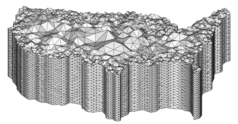
Figure 1: A space-time discontinuous Galerkin finite element mesh.

1 Introduction

Many simulation problems consider the behavior of an object or region of space over time. The most common finite element methods for this class of problem use a meshing procedure to discretize space, yielding a system of ordinary differential equations in time. A time-marching or time-integration scheme is then used to advance the solution over a series of fixed time steps. In general, a distinct spatial mesh may be required at each time step, due to the requirements of an adaptive analysis scheme or to track a moving boundary or interface within the domain.

A relatively new approach to such simulations suggests directly meshing in space-time [9, 16, 22]. For example, a four-dimensional space-time mesh would be required to simulate an evolving three-dimensional domain. Usually, the time dimension is not treated in the same way as the spatial dimensions, in part because it can be scaled independently. Moreover, the numerical methods that motivate our research impose additional geometric constraints on the meshes to support a linear-time solution strategy. Thus, traditional meshing techniques do not apply.

In this paper, we develop the first algorithm to build graded space-time meshes over arbitrary simplicially meshed domains in arbitrary dimensions. Our algorithm does not impose a fixed global time step on the mesh; rather, the duration of each space-time element depends on the local feature size and quality of the underlying space mesh. Our approach is a generalization of the ‘Tent Pitcher’ algorithm of Üngör and Sheffer [19], but avoids the restrictions of that method by imposing some additional constraints. Our algorithm builds space-time meshes in constant time per element.

The paper is organized as follows. In Section 2, we formalize the space-time meshing problem and describe several previous results. Section 3 explains the high-level advancing front strategy of our meshing algorithm. In Sections 4 and 5, we develop our algorithm for building three-dimensional space-time meshes over triangulated planar domains. We generalize our algorithm to higher dimensions in Section 6. In Section 7, we describe our implementation and present some experimental results. Finally, we conclude in Section 8 by suggesting several directions for further research.

2 Space-Time Discontinuous Galerkin Meshing

The formulation of our space-time meshing problem relies on the notions of domain of influence and domain of dependence. Imagine dropping a pebble into a pond; over time, circular waves expand outward from the point of impact. These waves sweep out a cone in space-time, called the domain of influence of the event.

More generally, we say that a point $\hat{p}$ in space-time depends on another point $\hat{q}$ if the salient physical parameters at $\hat{p}$ (temperature, pressure, stress, momentum, etc.) can depend on the corresponding parameters at $\hat{q}$, that is, if changing the conditions at $\hat{q}$ could change the conditions at $\hat{p}$. The domain of influence of $\hat{p}$ is the set of points that depend on $\hat{p}$; symmetrically, the domain of dependence is the set of points that $\hat{p}$ depends on. At least infinitesimally, these domains can be approximated by a pair of circular cones with common apex $\hat{p}$. For isotropic problems without material flow, this double cone can described by a scalar wave speed $c(\hat{p})\in\mathrm{I\!R}$, which specifies how quickly the radius of the cones grows as a function of time. If the characteristic equations of the analysis problem are linear and the material properties are homogeneous, the wave speed is constant throughout the entire space-time domain; in this case, we can choose an appropriate time scale so that ${c(\hat{p})=1}$ everywhere. For more general problems, the wave speed varies across space-time as a function of other physical parameters, and may even be part of the numerical solution.

These notions extend to finite element meshes in space-time. We say that an element $\triangle$ in space-time depends on another element $\triangle^{\prime}$ if any point $\hat{p}\in\triangle$ depends on any point $\hat{q}\in\triangle^{\prime}$. This relation naturally defines a directed dependency graph whose vertices are the elements of the mesh. Two elements in the mesh are coupled if they lie on a common directed cycle in (the transitive closure of) the dependency graph.

Space-time discontinuous Galerkin (DG) methods have been proposed by Richter [12], Lowrie et al. [9], and Yin et al. [22] for solving systems of nonlinear hyperbolic partial differential equations. These methods provide a linear-time element-by-element solution, avoiding the need to solve a large system of equations, provided no two elements in the underlying space-time mesh are coupled. In particular, every pair of adjacent elements must satisfy the so-called cone constraint: Any boundary facet between two neighboring elements separates the cone of influence from the cone of dependence of any point on the facet. See Figure 2. Intuitively, if a boundary facet satisfies the cone constraint, information can only flow in one direction across that facet. In a totally decoupled mesh, the dependency graph describes a partial order on the elements, and the solution can be computed by considering the elements one at a time according to any linear extension of this partial order. Alternatively, the solutions within any set of incomparable elements can be computed in parallel.

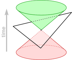
Figure 2: The cone constraint: Any boundary facet separates the domain of influence (above) from the domain of dependence (below).

Discontinuous Galerkin methods impose no a priori restrictions on the shape of the individual elements; mixed meshes with tetrahedral, hexahedral, pyramidal, and other element shapes are acceptable. However, it is usually more convenient to work with very simple convex elements such as simplices. Experience indicates that ill-conditioning is likely if the elements are non-convex, and subdividing non-convex regions into simple convex elements is useful for efficient integration. (For further background on DG methods, we refer the reader to the recent book edited by Cockburn, Karniadakis, and Shu [6], which contains both a general survey [5] and several papers describing space-time DG methods and their applications.)

To construct an efficient mesh with convex elements, we have found it preferable to relax the cone constraint in the following way. We construct a mesh of simplicial elements, but not all facets meet the cone constraint. Instead, elements are grouped into patches (of bounded size). The boundary facets between patches by definition satisfy the cone constraint, so patches are partially ordered by dependence, and can be solved independently.

However, the internal facets between simplicial elements within a patch may violate the cone constraint. Thus, DG methods require the elements within the patch to be solved simultaneously. Since each patch contains a constant number of elements, the system of equations within it has constant size, which implies that we can still solve the underlying numerical problem in linear time by considering the patches one at a time.

Richter [12] observed that the dissipation of DG methods increases as the slope of boundary facets decreases below the local wave speed. Thus, our goal is to construct an efficient simplicial mesh, grouped into patches each containing few simplices, such that the boundary facets of each patch are as close as possible to the cone constraint without violating it.

Previous Results

Most previous space-time meshing algorithms construct a single mesh layer between two space-parallel planes and repeat this layer (or its reflection) at regular intervals to fill the simulation domain. The exact construction method depends on the type of underlying space mesh. For example, given a structured quad space mesh, the space-time meshing algorithm of Lowrie et al. [9] constructs a layer of pyramids and tetrahedra. Similarly, Üngör et al. [18, 21] build a single layer of tetrahedra and pyramids over an acute triangular mesh, and Sheffer et al. [14, 21] describe an algorithm to build a single layer of hexahedra over any (unstructured) quad mesh. All such layer-based approaches suffer from a global time step imposed by the smallest element in the underlying space mesh. This requirement increases the number of elements in the mesh, making the DG method less efficient; it also increases the numerical error of the solution, since many internal facets must lie significantly below the constraint cone.

A few recent algorithms do not impose a global time step, but instead allows the durations of space-time elements to depend on the size of the underlying elements of the ground mesh. The first such algorithm, due to Üngör et al. [20], builds a triangular mesh for a $(1+1)$-dimensional space-time domain by intersecting the constraint cones at neighboring nodes. This method does not easily generalize to higher dimensions. The most general space-time meshing algorithm to date is the ‘Tent Pitcher’ algorithm of Üngör and Sheffer [19]. Given a simplicial space mesh in any fixed dimension, where every dihedral angle is strictly less than $90^{\circ}$, Tent Pitcher constructs a space-time mesh of arbitrary duration. Moreover, if every dihedral angle in the space mesh is larger than some positive constant, each patch in the space-time mesh consists of a constant number of simplices.

Unfortunately, the acute simplicial meshes that Tent Pitcher requires are difficult to construct, if not impossible, except in a few special cases. Bern et al. [2] describe two methods for building an acute triangular mesh for an arbitrary planar point set, and methods are known for special planar domains such as triangles [11], squares [3, 7], and some classes of polygons [8, 10]. However, no method is known for general planar domains or even for point sets in higher dimensions. It is an open problem whether the cube has an acute triangulation; see [17] for recent related results.

New Results

In this paper, we present a generalization of the Tent Pitcher algorithm that extends any simplicial space mesh in $\mathrm{I\!R}^{d}$, for any $d\geq 1$, into a space-time mesh of arbitrary duration. Like the Tent Pitcher algorithm, our algorithm does not rely on a single global time step. Our algorithm avoids the requirement of an acute ground mesh by carefully adapting the duration of space-time elements to the quality of the underlying simplices in the space mesh.

3 The Advancing Front

Our algorithm is designed as an advancing front procedure, which alternately constructs a patch of the mesh and invokes a space-time discontinuous Galerkin method to compute the required solution within that patch. To simplify the algorithm description, we assume that the wave speed is constant throughout space-time; specifically, by choosing an appropriate time scale, we will assume that $c(\hat{p})=1$ everywhere. Our algorithm can be easily adapted to handle changing wave speeds, provided the wave speed at any point is a non-increasing function of time. We discuss the necessary changes for non-constant wave speeds at the end of Section 5.

The input to our algorithm is a simplicial ground mesh $M$ of some spatial domain $X\subset\mathrm{I\!R}^{d}$, with the appropriate initial conditions stored at every element. The advancing front $\hat{M}$ is the graph of a continuous time function $t:X\to\mathrm{I\!R}$ whose restriction to any element of the ground mesh is linear. Any any stage of our algorithm, each element of the front satisfies the cone constraint $\mathopen{\|}\nabla t\mathclose{\|}\leq 1$. We will assume the initial time function is constant, but more general initial conditions are also permitted.

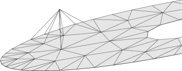
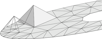
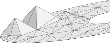
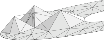
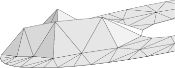
Figure 3: Pitching a series of tents over a planar triangulation.

To advance the front, our algorithm chooses a vertex that is a local minimum with respect to time, that is, a vertex $\hat{p}=(p,t(p))$ such that $t(p)\leq t(q)$ for every neighboring vertex $\hat{q}$. (Initially, every vertex on the front is a local minimum.) To obtain the new front, this vertex is moved forward in time to a new point $\hat{p}^{\prime}=(p,t^{\prime}(p))$ with $t^{\prime}(p)>t(p)$. We call the volume between the the old and new fronts a tent. The elements adjacent to $\hat{p}$ on the old front make up the inflow boundary of the tent; the corresponding elements on the new front comprise the patch’s outflow boundary. We decompose the tent into a patch of simplicial elements, all containing the common edge $\hat{p}\hat{p}^{\prime}$, and pass this patch, along with the physical parameters at its inflow boundary, to a DG solver. The solver returns the physical parameters for the outflow boundary, which we store for use as future inflow data. The solution parameters in the interior and inflow boundary of the tent can than be written to a file (for later analysis or visualization) and discarded. This advancing step is repeated until every node on the front passes some target time value.

If the front has several local minima, we could apply any number of heuristics for choosing one; Üngör and Sheffer outline several possibilities [19]. The correctness of our algorithm does not depend on which local minimum is chosen. In particular, if any vertex has the same time value as one of its neighbors, we can break the tie arbitrarily. Our implementation computes the mesh in phases. In each phase, we select a maximal independent set $S$ of local minima and then lift each minimum in $S$, in some arbitrary order. This approach seems particularly amenable to parallelization, since the minima in $S$ can be treated simultaneously by separate processors.

4 Pitching Just One Triangle

To complete the description of our algorithm, it remains only to describe how to compute the new time value for each vertex to be advanced, or less formally, how high to pitch each tent. We first consider the special case where the ground mesh consists of a single triangle. As we will show in the next section, this special case embodies all the difficulties of space-time meshing over general planar domains.

Let $p,q,r$ be three points in the plane. At any stage of our algorithm, the advancing front consists of a single triangle $\triangle\hat{p}\hat{q}\hat{r}$ whose vertices have time coordinates $t(p),t(q),t(r)$. Suppose without loss of generality that $t(p)<t(q)<t(r)$ and we want to advance $\hat{p}$ forward in time. We must choose the new time value $t^{\prime}(p)$ so that the resulting triangle $\triangle\hat{p}^{\prime}\hat{q}\hat{r}$ satisfies the cone constraint $\mathopen{\|}\nabla t\mathclose{\|}\leq 1$.

To simplify the derivation, suppose $q=(0,0)$ and $t(q)=0$. The time values $t^{\prime}(p)$ and $t(r)$ can then be written as $t^{\prime}(p)=p\cdot\nabla t$ and $t(r)=r\cdot\nabla t$, where $\nabla t$ is the gradient of the new time function. We can write this gradient vector as

$$\nabla t=\mu\bar{v}+\nu\bar{n},$$

where $\bar{v}$ is the unit vector parallel to the vector $r$, and $\bar{n}$ is the unit vector orthogonal to $\bar{v}$ with sign chosen so that $\bar{n}\cdot p>0$. The vector $\mu\bar{v}$ is just the gradient of the time function restricted to segment $qr$, so $\mu=t(r)/\mathopen{\|}r\mathclose{\|}$. The cone constraint implies that $\mathopen{\|}\nabla t\mathclose{\|}=\sqrt{\mu^{2}+\nu^{2}}\leq 1$ and therefore $\nu\leq\sqrt{1-\mu^{2}}$. Thus, the cone constraint is equivalent to the following inequality:

$$t^{\prime}(p) =p\cdot\nabla t$$

$$=\mu p\cdot\bar{v}+\nu p\cdot\bar{n}$$

$$\leq\mu p\cdot\bar{v}+\sqrt{1+\mu^{2}}\,p\cdot\bar{n}$$

$$=\frac{t(r)}{\mathopen{\|}r\mathclose{\|}}\,p\cdot\bar{v}+\frac{\sqrt{\mathopen{\|}r\mathclose{\|}^{2}-t(r)^{2}}}{\mathopen{\|}r\mathclose{\|}}\,p\cdot\bar{n}$$

$$=\frac{t(r)}{\mathopen{\|}r\mathclose{\|}^{2}}\,p\cdot r+\frac{\sqrt{\mathopen{\|}r\mathclose{\|}^{2}-t(r)^{2}}}{\mathopen{\|}r\mathclose{\|}^{2}}\,\mathopen{|}p\times r\mathclose{|}$$

Here, $p\times r$ denotes the two-dimensional cross product $p_{1}r_{2}-p_{2}r_{1}$, which is just twice the signed area of $\triangle{pqr}$. To simplify the notation slightly, let $w_{p}$ denote the distance from $p$ to $\mathord{\leftarrow}\mkern-6.0mu\cleaders\hbox{$\mkern-2.0mu\mathord{-}\mkern-2.0mu$}\hfill\mkern-6.0mu\mathord{\rightarrow}$ $\hfil\displaystyle{\,\vphantom{x}qr\,}\hfil$ , and define $w_{q}$ and $w_{r}$ analogously:

$$w_{p}=\frac{2\mathopen{|}\triangle pqr\mathclose{|}}{\mathopen{\|}r-q\mathclose{\|}},\quad w_{q}=\frac{2\mathopen{|}\triangle pqr\mathclose{|}}{\mathopen{\|}p-r\mathclose{\|}},\quad w_{r}=\frac{2\mathopen{|}\triangle pqr\mathclose{|}}{\mathopen{\|}q-p\mathclose{\|}}.$$

Then the previous inequality can be rewritten as

$$t^{\prime}(p)\leq\frac{t(r)}{\mathopen{\|}r\mathclose{\|}^{2}}\,p\cdot r+\frac{\sqrt{\mathopen{\|}r\mathclose{\|}^{2}-t(r)^{2}}}{\mathopen{\|}r\mathclose{\|}}\,w_{p}.$$ (1)

More generally, if $q\neq(0,0)$ and $t(q)\neq 0$, the cone constraint is equivalent to the following inequality.

$$\framebox{$\begin{array}[]{@{}r@{}l@{}}t^{\prime}(p)\leq{}t(q)&{}+{\displaystyle\frac{t(r)-t(q)}{\mathopen{\|}r-q\mathclose{\|}^{2}}}\,(p-q)\cdot(r-q)\\[12.91663pt] &{}+{\displaystyle\frac{\sqrt{\mathopen{\|}r-q\mathclose{\|}^{2}-(t(r)-t(q))^{2}}}{\mathopen{\|}r-q\mathclose{\|}}}\,w_{p}\end{array}$}$$ (2)

We have similar inequalities for every other ordered pair of vertices, limiting how far forward in time the lowest vertex can be moved past the middle vertex. We will collectively refer to these six inequalities as the cone constraint.

To ensure that our algorithm can create a mesh up to any desired time value, we must also maintain the following progress invariant:

The lowest vertex of $\triangle\hat{p}\hat{q}\hat{r}$ can always be lifted above the middle vertex without violating the cone constraint.

This invariant holds trivially at the beginning of the algorithm, when $t(p)=t(q)=t(r)=0$. Let us assume inductively that it holds at the moment we want to lift $\hat{p}$. Üngör and Sheffer [19] proved that if $\triangle pqr$ is acute, then satisfying the cone constraint automatically maintains this invariant, but for obtuse triangles, this is not enough.

To maintain our progress invariant, it suffices to ensure that in the next step of the algorithm, the new lowest vertex $\hat{q}$ can be lifted above $\hat{r}$ without violating the cone constraint. In other words, if we replace $t(q)$ with $t(r)$, the new triangle’s slope must be strictly less than $1$. By substituting $t(r)$ for $t(q)$ in the cone constraint (2) and making the inequality strict, we obtain the following:

$$\framebox{$t^{\prime}(p)<t(r)+w_{p}$}$$ (3)

We have similar inequalities for every other ordered pair of vertices, limiting how far forward in time the lowest vertex can be moved past the highest vertex. We will collectively refer to these six inequalities as the weak progress constraint.

The weak progress constraint has a simple geometric interpretation, which we can see by looking at the lifted triangle in space-time; see Figure 4. Let $\Gamma$ be the cone of dependence of the lifted point $\hat{p}^{\prime}$; this cone intersects the plane $t=t(r)$ in a circle $\gamma$ of radius ${t^{\prime}(p)-t(r)}$. Any plane $\pi$ through $\hat{p}^{\prime}$ that satisfies the cone constraint is disjoint from $\Gamma$; in particular, the intersection line of $\pi$ with the plane $t=t(r)$ does not cross $\gamma$. Now let $\hat{q}^{\prime}=(q,t(r))$. If the plane $\hat{p}^{\prime}\hat{q}^{\prime}\hat{r}$ satisfies the cone constraint, then the line through $\hat{q}^{\prime}$ and $\hat{r}$ does not cross $\gamma$. Thus, the progress invariant holds after we lift $\hat{p}$ only if $t^{\prime}(p)-t(r)<w_{p}$.

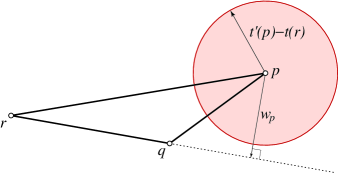
Figure 4: If the circle around $p$ does not touch the line through $q$ and $r$, then $\hat{q}$ can be lifted above $\hat{r}$ in the next step.

Our algorithm lifts $\hat{p}$ to some point $\hat{p}^{\prime}$ that satisfies both the cone constraint and the weak progress constraint, where $t^{\prime}(p)>t(q)$. By the progress invariant, this does not violate the cone constraint. If $t^{\prime}(p)\geq t(r)$, then the weak progress constraint implies that the progress invariant still holds. If $t^{\prime}(p)<t(r)$, then the progress invariant also still holds, because $t(r)-t^{\prime}(p)<t(r)-t(q)$. Thus, by induction, the progress invariant is maintained at every step of our algorithm.

Unfortunately, the weak progress constraint does not guarantee that we can reach any desired time value; in principle, the advancing front could converge to some finite limit. To guarantee significant progress at every step of the algorithm, we need a slightly stronger constraint. Our implementation uses the inequality

$$\framebox{$t^{\prime}(p)\leq t(r)+(1-\varepsilon)w_{p}$}$$ (4)

where $\varepsilon$ is a fixed constant in the range ${0<\varepsilon\leq 1/2}$. We have a similar inequality for every other ordered pair of vertices, and we collectively refer to these six inequalities as the progress constraint.

With this stronger constraint in place, we have the following result.

Lemma 1

If the cone constraint and progress constraint hold beforehand, we can lift $\hat{p}$ at least $\varepsilon w_{p}$ above $\hat{q}$ without violating either constraint.

• Without loss of generality, assume that $q=(0,0)$ and $t(q)=0$. We want to prove that setting $t^{\prime}(p)=\varepsilon w_{p}$ does not violate the cone constraint (in its simpler form (1)) or the progress constraint (4). Recall our assumption that $t(r)\geq t(q)=0$. Because $\varepsilon\leq 1/2$, we have

  $$t^{\prime}(p)=\varepsilon w_{p}\leq(1-\varepsilon)w_{p}\leq t(r)+(1-\varepsilon)w_{p},$$

  so the progress constraint is satisfied. The previous progress constraint implies that $t(r)\leq{(1-\varepsilon)w_{r}}$. Because $\varepsilon>0$ and $w_{r}\leq\mathopen{\|}r\mathclose{\|}=\mathopen{\|}r-q\mathclose{\|}$, we have

  $$t(r)^{2}\leq(1-\varepsilon)^{2}w_{r}^{2}\leq(1-\varepsilon^{2})\mathopen{\|}r\mathclose{\|}^{2},$$

  which implies that

  $$\varepsilon\leq\frac{\sqrt{\mathopen{\|}r\mathclose{\|}^{2}-t(r)^{2}}}{\mathopen{\|}r\mathclose{\|}}.$$

  Finally, because $t(r)\geq 0$, we have

  $$t^{\prime}(p)=\varepsilon w_{p} \leq\frac{\sqrt{\mathopen{\|}r\mathclose{\|}^{2}-t(r)^{2}}}{\mathopen{\|}r\mathclose{\|}}w_{p}$$

  $$\leq\frac{t(r)}{\mathopen{\|}r\mathclose{\|}^{2}}\,p\cdot r+\frac{\sqrt{\mathopen{\|}r\mathclose{\|}^{2}-t(r)^{2}}}{\mathopen{\|}r\mathclose{\|}}w_{p}.$$

  Thus, the cone constraint is also satisfied.  ${\square}$

Theorem 2

Given any three points $p,q,r\in\mathrm{I\!R}^{2}$, any real value $T>0$, and any constant $0<\varepsilon\leq 1/2$, our algorithm generates a tetrahedral mesh of the prism $\triangle pqr\times[0,T]$, where every internal facet satisfies the cone constraint. The number of tetrahedra is at most $TP/2A\varepsilon$, where $P$ is the perimeter and $A$ is the area of $\triangle pqr$.

• Our algorithm repeatedly lifts the lowest vertex of $\triangle\hat{p}\hat{q}\hat{r}$ to the largest time value satisfying the cone constraint (2), the progress constraint (4), and a termination constraint $t\leq T$. Each time we lift a point, our algorithm creates a new tetrahedron. By Lemma 1, a new point becomes the lowest vertex, so the algorithm halts only when all three vertices reach the target plane $t=T$. Moreover, whenever $t(p)\leq t(q)\leq t(r)$, the algorithm chooses a new time value $t^{\prime}(p)\geq t(q)+\varepsilon w_{p}\geq t(p)+\varepsilon w_{p}$, except possibly when $t^{\prime}(p)=T$. Thus, $\hat{p}$ is lifted at most $T/\varepsilon w_{p}=T\mathopen{\|}q-r\mathclose{\|}/2A\varepsilon$ times before the algorithm terminates.  ${\square}$

5 Arbitrary Planar Domains

We now extend our meshing algorithm to more complex planar domains. The input is a triangular ground mesh $M$ of some planar domain $X$. As we described in Section 3, our algorithm maintains a polyhedral front $\hat{M}$ with a lifted vertex $\hat{p}=(p,t(p))$ for every vertex ${p\in M}$. To advance the front, our algorithm chooses a local minimum vertex $\hat{p}$ and lifts it to a new point $\hat{p}^{\prime}=(p,t^{\prime}(p))$.

The new time value $t^{\prime}(p)$ is simply the largest value that satisfies the cone constraints and progress constraints for every triangle in the ground mesh that contains $p$. The chosen time value $t^{\prime}(p)$ is the value that would be chosen by at least one of these triangles in isolation. It follows that $\hat{p}^{\prime}$ is not a local minimum in the modified front. Moreover, by our earlier arguments, the progress invariant is maintained in every triangle adjacent to $p$. It follows immediately that our algorithm can generate meshes to any desired time value.

Specifically, let $\omega_{p}$ denote the minimum distance from $p$ to $\mathord{\leftarrow}\mkern-6.0mu\cleaders\hbox{$\mkern-2.0mu\mathord{-}\mkern-2.0mu$}\hfill\mkern-6.0mu\mathord{\rightarrow}$ $\hfil\displaystyle{\,\vphantom{x}qr\,}\hfil$ , over all triangles $\triangle pqr$ in the ground mesh. Lemma 1 implies the following result.

Theorem 3

Given any triangular mesh $M$ over any domain $X\subset\mathrm{I\!R}^{2}$, any real value $T>0$, and any constant $0<\varepsilon\leq 1/2$, our algorithm generates a space-time mesh for the domain $X\times[0,T]$. The number of patches is at most $(T/\varepsilon)\sum_{p\in M}1/\omega_{p}$, and number of tetrahedra is at most $(6T/\varepsilon)\sum_{p\in M}1/\omega_{p}$.

Our analysis of the number of patches and elements is conservative, since it assumes that each step of the algorithm advances a vertex by the minimum amount guaranteed by Lemma 1. We expect most advances to be larger in practice, especially in areas of the ground mesh without large angles. Our experiments were consistent with this intuition; see Section 7.

Most of the parameters of the cone constraint, and all of the parameters of the progress constraint, can be computed in advance from the ground mesh alone. Thus, the time to compute each new time value $t^{\prime}(p)$ is a small constant times the degree of $p$ in the ground mesh, and the overall time required to build the mesh is a small constant times the number of mesh elements.

Non-constant Wave Speeds

Although we have described our algorithm under the assumption that the wave function $c(\hat{p})$ is constant, this assumption is not necessary. If elements of the ground mesh have different (but still constant) wave speeds, our algorithm requires only trivial modifications. The situation fits well with discontinuous Galerkin methods, which compute solutions with discontinuities at element boundaries. If the wave speed varies within a single element, even discontinuously, the only necessary modification is to compute and use the maximum wave speed over each entire element. Similar modifications suffice if the wave speed at any point in space can decrease over time.

If the mesh has only acute angles, the progress constraint is redundant and arguments of Üngör and Sheffer [19] imply that our algorithm works even if the wave speed can increase over time, as long as the wave speed is Lipschitz continuous. Unfortunately, their analysis breaks down for obtuse meshes because of the progress constraint, and indeed our algorithm can get stuck. We expect that a refinement of our progress constraint would allow for increasing wave speeds, but further study is required.

6 Higher Dimensions

Our meshing algorithm extends in an inductive manner to simplicial meshes in higher dimensions. As in the two-dimensional case, it suffices to consider the case where the ground mesh consists of a single simplex $\triangle$ in $\mathrm{I\!R}^{d}$. At each step of our algorithm, we increase the time value of the lowest of the simplex’s $d+1$ vertices as much as possible so that the cone constraint $\mathopen{\|}\nabla t\mathclose{\|}\leq 1$ is satisfied and we can continue inductively as far into the future as we like.

Let $p,q,r_{1},r_{2},\dots,r_{d-1}$ denote the vertices of $\triangle$ in increasing time order, breaking ties arbitrarily. Our goal is to lift $\hat{p}$ above $\hat{q}$ without violating the cone constraint. Let $F$ be the facet of $\triangle$ that excludes $p$, and let $H$ be the hyperplane spanning $F$. Let $p_{\!{}_{H}}\!$ be the projection of $p$ onto $H$, and let $p_{\!{}_{F}}\!$ be the closest point in $F$ to $p$. Observe that $\angle pp_{\!{}_{H}}\!p_{\!{}_{F}}\!$ is a right angle. See Figure 5. Let $\nabla_{\!\!{}_{H}}t$ denote the gradient vector of the time function restricted to $H$. Finally, define

$$\sigma_{\!{}_{F}}\!=\frac{\mathopen{\|}p-p_{\!{}_{H}}\!\mathclose{\|}}{\mathopen{\|}p-p_{\!{}_{F}}\!\mathclose{\|}}.$$

If $p_{\!{}_{H}}\!$ lies inside $F$, then $p_{\!{}_{H}}\!=p_{\!{}_{F}}\!$ and $\sigma_{\!{}_{F}}\!=1$; otherwise, $p_{\!{}_{H}}\!\neq p_{\!{}_{F}}\!$ and $\sigma_{\!{}_{F}}\!=\sin\angle p_{\!{}_{H}}\!p_{\!{}_{F}}\!p$.

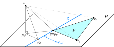
Figure 5: Defining the points $p_{\!{}_{H}}\!$, $p_{\!{}_{F}}\!$, and $p_{\!{}_{Z}}\!$

The higher-dimensional analogue of the weak progress constraint is described by the following lemma.

Lemma 4

If $\mathopen{\|}\nabla_{\!\!{}_{H}}t\mathclose{\|}<\sigma_{\!{}_{F}}\!$, then we can lift $\hat{p}$ above $\hat{q}$ without violating the cone constraint $\mathopen{\|}\nabla t\mathclose{\|}\leq 1$.

• Suppose $\mathopen{\|}\nabla_{\!\!{}_{H}}t\mathclose{\|}<\sigma_{\!{}_{F}}\!$. Without loss of generality, assume that $q=(0,0,\dots,0)$ and $t(q)=0$. Let $\bar{n}$ be the unit normal vector of $H$ with $p\cdot\bar{n}>0$,

  $$\bar{n}=\frac{p-p_{\!{}_{H}}\!}{\mathopen{\|}p-p_{\!{}_{H}}\!\mathclose{\|}}.$$

  Since the time function $t$ is linear, changing only $t(p)$ is equivalent to leaving $t$ fixed on the hyperplane $H$ and changing the directional derivative $\partial t/\partial\bar{n}$. To prove the lemma, we show that setting

  $$\frac{\partial t}{\partial\bar{n}}=\cos\angle p_{\!{}_{H}}\!p_{\!{}_{F}}\!p=\frac{\mathopen{\|}p_{\!{}_{H}}\!-p_{\!{}_{F}}\!\mathclose{\|}}{\mathopen{\|}p-p_{\!{}_{F}}\!\mathclose{\|}}$$ (5)

  gives us a new time function that satisfies the cone constraint with $t(p)>0$.

  Let $Z$ be the set of points in $H$ where $t=0$. Since $t(q)=0$, $Z$ is the $(d-2)$-flat orthogonal to $\nabla_{\!\!{}_{H}}t$ that passes through $q$. Moreover, because $t\geq 0$ everywhere in $F$, $Z$ is a supporting $(d-2)$-flat of $F$. Let $p_{\!{}_{Z}}\!$ be the closest point in $Z$ to $p$ (or to $p_{\!{}_{H}}\!$); this might be the same point as $p_{\!{}_{F}}\!$, $p_{\!{}_{H}}\!$, or $q$. Observe that $\angle pp_{\!{}_{H}}\!p_{\!{}_{Z}}\!$ is a right angle. See Figure 5.

  We can express the time gradient $\nabla t$ as follows:

  $$\nabla t=\nabla_{\!\!{}_{H}}t+\frac{\partial t}{\partial\bar{n}}\bar{n}.$$

  Equation (5) implies that

  $$\nabla t=\nabla_{\!\!{}_{H}}t+\frac{\mathopen{\|}p_{\!{}_{H}}\!-p_{\!{}_{F}}\!\mathclose{\|}}{\mathopen{\|}p-p_{\!{}_{F}}\!\mathclose{\|}}\bar{n}.$$

  Since these two components of $\nabla t$ are orthogonal, we can express its length as follows.

  $$\mathopen{\|}\nabla t\mathclose{\|}^{2} =\mathopen{\|}\nabla_{\!\!{}_{H}}t\mathclose{\|}^{2}+\frac{\mathopen{\|}p_{\!{}_{H}}\!-p_{\!{}_{F}}\!\mathclose{\|}^{2}}{\mathopen{\|}p-p_{\!{}_{F}}\!\mathclose{\|}^{2}}$$

  $$<\frac{\mathopen{\|}p-p_{\!{}_{H}}\!\mathclose{\|}^{2}}{\mathopen{\|}p-p_{\!{}_{F}}\!\mathclose{\|}^{2}}+\frac{\mathopen{\|}p_{\!{}_{H}}\!-p_{\!{}_{F}}\!\mathclose{\|}^{2}}{\mathopen{\|}p-p_{\!{}_{F}}\!\mathclose{\|}^{2}}=1$$

  So the new time function satisfies the cone constraint.

  We can express the time value $t(p)$ as follows:

  $$t(p) =t(p_{\!{}_{H}}\!)+\mathopen{\|}p-p_{\!{}_{H}}\!\mathclose{\|}\frac{\partial t}{\partial\bar{n}}$$

  $$=t(p_{\!{}_{H}}\!)+\frac{\mathopen{\|}p-p_{\!{}_{H}}\!\mathclose{\|}\,\mathopen{\|}p_{\!{}_{H}}\!-p_{\!{}_{F}}\!\mathclose{\|}}{\mathopen{\|}p-p_{\!{}_{F}}\!\mathclose{\|}}$$

  If $t(p_{\!{}_{H}}\!)\geq 0$, then clearly $t(p)>0$. Suppose ${t(p_{\!{}_{H}}\!)<0}$. The vector $p_{\!{}_{H}}\!-p_{\!{}_{Z}}\!$ is orthogonal to $Z$ and therefore anti-parallel to $\nabla_{\!\!{}_{H}}t$. Thus,

  $$t(p_{\!{}_{H}}\!) =\nabla_{\!\!{}_{H}}t\cdot(p_{\!{}_{H}}\!-p_{\!{}_{Z}}\!)$$

  $$=-\mathopen{\|}\nabla_{\!\!{}_{H}}t\mathclose{\|}\,\mathopen{\|}p_{\!{}_{H}}\!-p_{\!{}_{Z}}\!\mathclose{\|}$$

  $$\geq-\frac{\mathopen{\|}p-p_{\!{}_{H}}\!\mathclose{\|}\,\mathopen{\|}p_{\!{}_{H}}\!-p_{\!{}_{Z}}\!\mathclose{\|}}{\mathopen{\|}p-p_{\!{}_{F}}\!\mathclose{\|}}$$

  $$\geq-\frac{\mathopen{\|}p-p_{\!{}_{H}}\!\mathclose{\|}\,\mathopen{\|}p_{\!{}_{H}}\!-p_{\!{}_{F}}\!\mathclose{\|}}{\mathopen{\|}p-p_{\!{}_{F}}\!\mathclose{\|}}.$$

  The last inequality follows from the fact that $p_{\!{}_{H}}\!$ and $F$ lie on opposite sides of $Z$, because $t(p_{\!{}_{H}}\!)<0$. It now immediately follows that $t(p)>0$.  ${\square}$

As in the two-dimensional case, in order to guarantee that the algorithm does not converge prematurely, we must strengthen this constraint. There are many effective ways to do this; the following lemma describes one such method.

Lemma 5

For any $0<\varepsilon\leq 1$, if $\mathopen{\|}\nabla_{\!\!{}_{H}}t\mathclose{\|}\leq(1-\varepsilon)\sigma_{\!{}_{F}}\!$, then we can lift $\hat{p}$ at least $\varepsilon\mathopen{\|}p-p_{\!{}_{H}}\!\mathclose{\|}$ above $\hat{q}$ without violating the cone constraint $\mathopen{\|}\nabla t\mathclose{\|}\leq 1$.

• We modify the previous proof as follows. We show that setting

  $$\frac{\partial t}{\partial\bar{n}}=\varepsilon+(1-\varepsilon)\frac{\mathopen{\|}p_{\!{}_{H}}\!-p_{\!{}_{F}}\!\mathclose{\|}}{\mathopen{\|}p-p_{\!{}_{F}}\!\mathclose{\|}}$$

  gives us a new time function satisfying the conditions of the lemma. First we verify that the cone constraint is satisfied.

  $$\mathopen{\|}\nabla t\mathclose{\|}^{2} \leq\left((1-\varepsilon)\frac{\mathopen{\|}p-p_{\!{}_{H}}\!\mathclose{\|}}{\mathopen{\|}p-p_{\!{}_{F}}\!\mathclose{\|}}\right)^{2}+\left(\varepsilon+(1-\varepsilon)\frac{\mathopen{\|}p_{\!{}_{H}}\!-p_{\!{}_{F}}\!\mathclose{\|}}{\mathopen{\|}p-p_{\!{}_{F}}\!\mathclose{\|}}\right)^{2}$$

  $$=1+2\varepsilon(1-\varepsilon)\left(\frac{\mathopen{\|}p_{\!{}_{H}}\!-p_{\!{}_{F}}\!\mathclose{\|}}{\mathopen{\|}p-p_{\!{}_{F}}\!\mathclose{\|}}-1\right)$$

  $$\leq 1$$

  (In fact, if $p_{\!{}_{H}}\!\neq p_{\!{}_{F}}\!$, then $\mathopen{\|}\nabla t\mathclose{\|}<1$, which means we could lift $\hat{p}$ even more.)

  Next we verify that $t(p)\geq\varepsilon\mathopen{\|}p-p_{\!{}_{H}}\!\mathclose{\|}$.

  $$t(p) =t(p_{\!{}_{H}}\!)+\mathopen{\|}p-p_{\!{}_{H}}\!\mathclose{\|}\frac{\partial t}{\partial\bar{n}}$$

  $$=t(p_{\!{}_{H}}\!)+\varepsilon\mathopen{\|}p-p_{\!{}_{H}}\!\mathclose{\|}+(1-\varepsilon)\frac{\mathopen{\|}p-p_{\!{}_{H}}\!\mathclose{\|}\,\mathopen{\|}p_{\!{}_{H}}\!-p_{\!{}_{F}}\!\mathclose{\|}}{\mathopen{\|}p-p_{\!{}_{F}}\!\mathclose{\|}}$$

  $$\geq t(p_{\!{}_{H}}\!)+\varepsilon\mathopen{\|}p-p_{\!{}_{H}}\!\mathclose{\|}.$$

  If $t(p_{\!{}_{H}}\!)\geq 0$, we are done. Otherwise, as in the previous lemma, we have

  $$t(p_{\!{}_{H}}\!) \geq-\mathopen{\|}\nabla_{\!\!{}_{H}}t\mathclose{\|}\,\mathopen{\|}p_{\!{}_{H}}\!-p_{\!{}_{F}}\!\mathclose{\|}$$

  $$\geq-(1-\varepsilon)\frac{\mathopen{\|}p-p_{\!{}_{H}}\!\mathclose{\|}\,\mathopen{\|}p_{\!{}_{H}}\!-p_{\!{}_{F}}\!\mathclose{\|}}{\mathopen{\|}p-p_{\!{}_{F}}\!\mathclose{\|}},$$

  which immediately implies that $t(p)\geq\varepsilon\mathopen{\|}p-p_{\!{}_{H}}\!\mathclose{\|}$, as claimed.  ${\square}$

An important insight is that we can view the simplex $\triangle$ simultaneously as a single $d$-dimensional simplex and as $(d-1)$-dimensional boundary mesh. Lemma 5 prescribes a tighter cone constraint for every element in this boundary mesh.

Our algorithm proceeds as follows. At each step, we lift the lowest vertex of $\triangle$ by recursively applying the $(d-1)$-dimensional algorithm; then, if necessary, we lower the newly-lifted vertex to satisfy the global cone constraint $\mathopen{\|}\nabla t\mathclose{\|}\leq 1$. The base case of the dimensional recursion is the two-dimensional algorithm in the previous section.

This recursion imposes an upper bound on the length of the time gradient within every face of $\triangle$ of dimension at least $1$. In fact, a naïve recursive implementation would calculate $(d-k)!$ different constraints for each $k$-dimensional face. A more careful implementation would determine the strictest constraint for each face in an initialization phase, so that each step of the algorithm only needs to consider each face incident to the lifted vertex once.

For a $d$-dimensional ground mesh with more than one simplex, we apply precisely the same strategy as in the two-dimensional case. At each step of the algorithm, we choose an arbitrary local minimum vertex $\hat{p}$, and lift it to the highest time point $\hat{p}^{\prime}$ allowed by all the simplices (of all dimensions) containing $\hat{p}$. By our earlier arguments, $\hat{p}^{\prime}$ is not a local minimum of the modified front, which implies that our algorithm terminates only when all the vertices reach the target time value.

7 Output Examples

We have implemented our planar space-time meshing algorithm and tested it on several different ground meshes. Our implementation consists of approximately 5000 lines of C++ code, about 800 of which represent the actual space-time meshing algorithm; the remaining code is a pre-existing library for manipulating and visualizing triangular and tetrahedral meshes.

Figures 1 and 6–8 show space-time meshes computed by our implementation. In each case, we stopped advancing each vertex of the front after it passed a target time value. In every example, the input triangle mesh contains at least one (sometimes extremely) obtuse triangle, which caused Üngör and Sheffer’s original Tent Pitcher algorithm to fail [19].

Our program produces several thousand elements per second, running on a 1.7 GHz Pentium IV with 1 gigabyte of memory. For example, the mesh in Figure 1, which contains 114,515 tetrahedral elements, was built from a ground mesh of 2,356 triangles in about 14 seconds. Figure 6 shows an input mesh with 1,044 triangles and the resulting 55,020-element space-time mesh, which was computed in about 4 seconds. (These running times include reading and parsing the input mesh file and writing the output mesh to disk.)

(a)

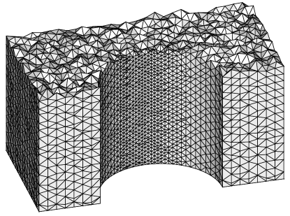
(b)

Figure 6: (a) A typical planar mesh of 1044 triangles. (b) The resulting space-time mesh of 55,020 tetrahedra, computed by our implementation in about 4 seconds.

Figure 7 illustrates effect of grading in the input mesh on the size on space-time elements. The largest and smallest elements in the ground mesh differ in size by a factor of 128; the resulting space-time elements differ in duration by a factor of 450. (The difference between these two factors might be explained by the obtuse triangles near the smallest element of the ground mesh.) Less severe grading due to varying ground element size can also be seen in Figure 6.

(a)

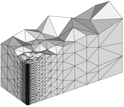
(b)

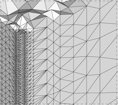
(c)

Figure 7: (a) A severely graded planar mesh. (b) The resulting space-time mesh. (c) A close-up of the resulting grading.

Figure 8 shows the output of our algorithm when the input mesh is pathological. The input meshes are the Delaunay triangulation and a greedy sweep-line triangulation of the same point set. As expected, variations in quality in the ground mesh also leads to temporal grading in our output meshes. For example, the bottom right vertex of the space mesh in Figure 8(b) advances much more quickly than the top right vertex, because it is significantly further from the lines through any of its neighboring edges.

We tried several different values of the parameter $\varepsilon$ in the progress constraint (4). All of the example output meshes were computed using the value $\varepsilon\approx 0.1$. Somewhat to our surprise, the number of elements in the output mesh varied by only a few percent as we varied $\varepsilon$ from $1/100$ to $1/3$, and smaller values of $\varepsilon$ usually resulted in meshes with slightly fewer elements, since the modified progress constraint is less severe. Also, for high-quality ground meshes, where most of the triangles are acute, the progress constraint affected only a few isolated portions of the space-time mesh. On the other hand, smaller values of $\varepsilon$ generally led to wider variability in the duration of neighboring tetrahedra. As $\varepsilon$ increases, the progress guaranteed by Lemma 1 more closely matches the maximum progress allowed by the progress constraint; this tends to distribute the progress of each triangle more evenly among its vertices.

8 Further Research

We have presented the first algorithm to generate graded space-time meshes for arbitrary spatial domains, suitable for efficient use by space-time discontinuous Galerkin methods. This is only the first step toward building a general space-time DG meshing library.

As we mentioned in Section 5, our algorithm currently requires the wave speed at any point in space to remain constant or monotonically decrease over time. In the short term, we plan to adapt our algorithm to handle wave speeds that increase over time. It should be noted that for many problems, the wave speed is not known in advance but must be computed on the fly as part of the numerical solution.

DG methods do not require conforming meshes, where any pair of adjacent elements meet in a common face. As a result, fixed time-step methods allow the space mesh to be refined or coarsened in response to error estimates, simply by remeshing at any time slice. Can our advancing front method be modified to allow for refinement, coarsening, or other local remeshing operations (like Delaunay flips)? These operations might be useful not only to avoid numerical error, but also to make the meshing process itself more efficient.

For many problems, even the boundary of the domain changes over time according to the underlying system of PDEs. Can our method be adapted to handle moving boundaries? Intuitively, we would like a mesh that conforms to the boundary as it moves. This would require us to move the nodes of the ground mesh continuously over time; remeshing operations would be required to guarantee that the meshing algorithm does not get stuck. Similar issues arise in tracking shocks, which are surfaces in space-time where the solution changes discontinuously.

Our method currently assumes that all the characteristic cone have vertical (or at least parallel) axes. For problems involving fluid flow, the direction of the cone axis (i.e., the velocity of the material) varies over space-time as part of the solution. We could adapt our method to this setting by overestimating the true tilted influence cones by larger parallel cones, but intuitively it seems more efficient to move nodes on the front. As in the case of moving boundaries, this would require remeshing the front. In fact, the front would no longer necessarily be a monotone polyhedral surface; extra work may be required to ensure that the resulting mesh is acyclic.

(a)	(b)
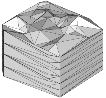
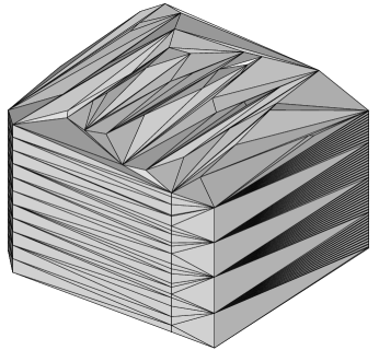
(c)	(d)

Figure 8: (a) A Delaunay triangulation with a few bad triangles. (b) A sweep-line triangulation (of the same point set) with many horrible triangles. (c,d) The resulting space-time meshes, showing the resulting temporal grading.

Finally, to minimize numerical error it is important to generate space-time meshes of high quality. Although there are several possible measures for the quality of a space-time element, further mathematical analysis of space-time DG methods is required to determine the most useful quality measures. This is in stark contrast to the traditional setting, where appropriate measures of quality and algorithms to compute high-quality meshes are well known [1, 2, 4, 13, 15].

Acknowledgments

The authors thank David Bunde, Michael Garland, Shripad Thite, and especially Bob Haber for several helpful comments and discussions.

This work was partially supported by NSF ITR grant DMR-0121695. Jeff Erickson was also partially supported by a Sloan Fellowship and NSF CAREER award CCR-0093348. Damrong Guoy was also partially supported by DOE grant LLNL B341494. John Sullivan was also partially supported by NSF grant DMS-00-71520. Alper Üngör was also partially supported by a UIUC Computational Science and Engineering Fellowship.

References

- [1] M. Bern, L. P. Chew, D. Eppstein, and J. Ruppert. Dihedral bounds for mesh generation in high dimensions. Proc. 6th Annu. ACM-SIAM Sympos. Discrete Algorithms, 89–196, 1995.
- [2] M. Bern, D. Eppstein, and J. Gilbert. Provably good mesh generation. J. Comput. System Sci. 48:384–409, 1994.
- [3] C. Cassidy and G. Lord. A square acutely triangulated. J. Rec. Math. 13(4):263–268, 1980.
- [4] S.-W. Cheng, T. K. Dey, H. Edelsbrunner, M. A. Facello, and S.-H. Teng. Sliver exudation. Proc. 15th Annu. ACM Sympos. Comput. Geom., 1–13. 1999.
- [5] B. Cockburn, G. Karniadakis, and C. Shu. The development of discontinuous Galerkin methods. Discontinuous Galerkin Methods: Theory, Computation and Applications, pp. 1–14. Lecture Notes Comput. Sci. Engin. 11, Springer, 2000.
- [6] B. Cockburn, G. Karniadakis, and C. Shu. Discontinuous Galerkin Methods: Theory, Computation and Applications. Lecture Notes Comput. Sci. Engin. 11, Springer, 2000.
- [7] D. Eppstein. Acute square triangulation. The Geometry Junkyard, July 1997. http://www.ics.uci.edu/~eppstein/junkyard/acute-square/.
- [8] T. Hangan, J. Itoh, and T. Zamfirescu. Acute triangulations. Bulletin Math. de la Soc. des Sci. Math. de Roumanie 43:279–286, 2000.
- [9] R. B. Lowrie, P. L. Roe, and B. van Leer. Space-time methods for hyperbolic conservation laws. Barriers and Challenges in Computational Fluid Dynamics, pp. 79–98. ICASE/LaRC Interdisciplinary Series in Science and Engineering 6, Kluwer, 1998.
- [10] H. Maehara. On acute triangulations of quadrilaterals. Proc. Japan Conf. Discrete Comput. Geom., pp. 237–243. Lecture Notes Comput. Sci. 2098, Springer-Verlag, 2000. http://link.springer.de/link/service/series/0558/bibs/2098/20980237.htm.
- [11] W. Manheimer. Solution to problem E1406: Dissecting an obtuse triangle into acute triangles. Amer. Math. Monthly 67, 1960.
- [12] G. R. Richter. An explicit finite element method for the wave equation. Applied Numer. Math. 16:65–80, 1994.
- [13] J. Ruppert. A Delaunay refinement algorithm for quality 2-dimensional mesh generation. J. Algorithms 18(3); 548–585, 1995.
- [14] A. Sheffer, A. Üngör, S.-H. Teng, and R. B. Haber. Generation of 2D space-time meshes obeying the cone constraint. Advances in Computational Engineering & Sciences, pp. 1360–1365. Tech Science Press, 2000.
- [15] J. R. Shewchuk. Tetrahedral mesh generation by Delaunay refinement. Proc. 14th Annu. ACM Sympos. Comput. Geom., 86–95, 1998.
- [16] L. L. Thompson. Design and Analysis of Space-Time and Galerkin Least-Squares Finite Element Methods for Fluid-Structure Interaction in Exterior Domains. Ph.D. thesis, Stanford University, 1994.
- [17] A. Üngör. Tiling 3D Euclidean space with acute tetrahedra. Proc. 13th Canadian Conf. Comput. Geom., 169–172, 2001. http://compgeo.math.uwaterloo.ca/~cccg01/proceedings/
- [18] A. Üngör, C. Heeren, X. Li, A. Sheffer, R. B. Haber, and S.-H. Teng. Constrained 2D space-time meshing with all tetrahedra. Proc. 16th IMACS World Congress, 2000.
- [19] A. Üngör and A. Sheffer. Pitching tents in space-time: Mesh generation for discontinuous Galerkin method. Proc. 9th Int. Meshing Roundtable, 111–122, 2000. http://www.andrew.cmu.edu/user/sowen/abstracts/Un738.html.
- [20] A. Üngör, A. Sheffer, and R. B. Haber. Space-time meshes for nonlinear hyperbolic problems satisfying a nonuniform angle constraint. Proc. 7th Int. Conf. Numerical Grid Generation in Computational Field Simulations, 2000.
- [21] A. Üngör, A. Sheffer, R. B. Haber, and S.-H. Teng. Layer based solutions for constrained space-time meshing. To appear in Applied Numer. Math., 2002. http://www.cse.uiuc.edu/~ungor/abstracts/layerAPNUM.html.
- [22] L. Yin, A. Acharya, N. Sobh, R. Haber, and D. A. Tortorelli. A space-time discontinuous Galerkin method for elastodynamic analysis. Discontinuous Galerkin Methods: Theory, Computation and Applications, pp. 459–464. Lecture Notes Comput. Sci. Engin. 11, Springer, 2000.