Effectiveness of preference elicitation in combinatorial auctions

Abstract

Combinatorial auctions where agents can bid on bundles of items are desirable because they allow the agents to express complementarity and substitutability between the items. However, expressing one’s preferences can require bidding on all bundles. Selective incremental preference elicitation by the auctioneer was recently proposed to address this problem [4], but the idea was not evaluated. In this paper we show, experimentally and theoretically, that automated elicitation provides a drastic benefit. In all of the elicitation schemes under study, as the number of items for sale increases, the amount of information elicited is a vanishing fraction of the information collected in traditional “direct revelation mechanisms” where bidders reveal all their valuation information. Most of the elicitation schemes also maintain the benefit as the number of agents increases. We develop more effective elicitation policies for existing query types. We also present a new query type that takes the incremental nature of elicitation to a new level by allowing agents to give approximate answers that are refined only on an as-needed basis. In the process, we present methods for evaluating different types of elicitation policies.

1 Introduction

Combinatorial auctions, where agents can submit bids on bundles of items, are economically efficient mechanisms for selling $k$ items to $n$ bidders, and are attractive when the bidders’ valuations on bundles exhibit complementarity (a bundle of items is worth more than the sum of its parts) and/or substitutability (a bundle is worth less than the sum of its parts). Determining the winners in such auctions is a complex optimization problem that has recently received considerable attention (e.g., [19, 24, 7, 13, 1, 25, 26, 6, 9]).

An equally important problem, which has received much less attention, is that of bidding. There are $2^{k}-1$ bundles, and each agent may need to bid on all of them to fully express its preferences. This can be undesirable for any of several reasons: determining one’s valuation for any given bundle can be computationally intractable [21, 16, 11, 23, 10]; there is a huge number of bundles to evaluate; communicating the bids can incur prohibitive overhead (e.g., network traffic); and agents may prefer not to reveal all of their valuation information due to reasons of privacy or long-term competitiveness [20]. Appropriate bidding languages [24, 7, 22, 13, 9] can solve the communication overhead in some cases (when the bidder’s utility function is compressible). However, they still require the agents to completely determine and transmit their valuation functions and as such do not solve all the issues. So in practice, when the number of items for sale is even moderate, the bidders will not bid on all bundles. Instead, they may wastefully bid on bundles which they will not win, and they may suffer reduced economic efficiency by failing to bid on bundles they would have won.

Selective incremental preference elicitation by the auctioneer was recently proposed to address these problems [4], but the idea was not evaluated. We implemented the most promising elicitation schemes from that paper, starting from a rigid search-based scheme and continuing to a general flexible elicitation framework. We evaluated the previous schemes, and also developed a host of new elicitation policies. Our experiments show that elicitation reduces revelation drastically, and that this benefit increases with problem size. We also provide theoretical results on elicitation policies. Finally, we introduce and evaluate a new query type that takes the incremental nature of elicitation to a new level by allowing agents to give approximate answers that are refined only on an as-needed basis.

2 Auction and elicitation setting

We model the auction as having a single auctioneer selling a set $K$ of items to $n$ bidder agents (let $k=|K|$). Each agent $i$ has a valuation function $v_{i}:2^{K}\mapsto\mathbb{R}$ that determines a finite private value $v_{i}(b)$ for each bundle $b\subseteq K$. We make the usual assumption that the agents have free disposal, that is, adding items to an agent’s bundle never makes the agent worse off because, at worst, the agent can dispose of extra items for free. Formally, $\forall b\subseteq K,b^{\prime}\subseteq b$, $v_{i}(b)\geq v_{i}(b^{\prime})$. The techniques of the paper could also be used without free disposal, although more elicitation would be required due to less a priori structure.

At the start of the auction, the auctioneer knows the items and the agents, but has no information about the agents’ value functions over the bundles—except that the agents have free disposal. The auction proceeds by having the auctioneer incrementally elicit value function information from the agents one query at a time until the auctioneer has enough information to determine an optimal allocation of items to agents. Therefore, we also call the auctioneer the elicitor. An allocation is optimal if it maximizes social welfare $\sum_{i=1}^{n}v_{i}(b_{i})$, where $b_{i}$ is the bundle that agent $i$ receives in the allocation. The goal of the elicitor is to determine an optimal allocation with as little elicitation as possible. A recent theoretical result shows that even with free disposal, in the worst case, finding an (even only approximately) optimal allocation requires exponential communication [14]. Therefore, we will judge the techniques successful if they reduce communication from full revelation by an asymptotic amount.

3 Elicitor’s inference and constraint network

The elicitor, as we designed it, never asks a query whose answer could be inferred from the answers to previous queries. To support the storing and propagation of information received from the agents, we have the elicitor store its information in a constraint network. Specifically, the elicitor stores a graph for each agent. In each graph, there is one node for each bundle $b$. Each node is labeled by an interval $[\textit{LB}_{i}(b),\textit{UB}_{i}(b)]$. The lower bound $\textit{LB}_{i}(b)$ is the highest lower bound the elicitor can prove on the true $v_{i}(b)$ given the answers received to queries so far. Analogously, $\textit{UB}_{i}(b)$ is the lowest upper bound. We say a bound is tight when it is equal to the true value.

Each graph can also have directed edges. A directed edge $(a,b)$ encodes the knowledge that the agent prefers bundle $a$ over bundle $b$ (that is, $v_{i}(a)\geq v_{i}(b)$). The elicitor may know this even without knowing $v_{i}(a)$ or $v_{i}(b)$. An edge $(a,b)$ lets the elicitor infer that $\textit{LB}_{i}(a)\geq\textit{LB}_{i}(b)$, which allows it to tighten the lower bound on $a$ and on any of $a$’s ancestors in the graph. Similarly, the elicitor can infer $\textit{UB}_{i}(a)\geq\textit{UB}_{i}(b)$, which allows it to tighten the upper bound on $b$ and its descendants in the graph.

We define the relation $a\succeq b$ (read “$a$ dominates $b$”) to be true if we can prove that $v_{i}(a)\geq v_{i}(b)$. This is the case either if $\textit{LB}_{i}(a)\geq\textit{UB}_{i}(b)$, or if there is a directed path from $a$ to $b$ in the graph. The free disposal assumption allows the elicitor to infer the following dominance relations before the elicitation begins: $\forall b\subseteq K,b^{\prime}\subseteq b$, $b\succeq b^{\prime}$.

Because the $\succeq$ relation is transitive, to encode the free disposal constraints, we only need to add edges from each bundle $a$ to the bundles $b$ that include all but one item in $a$. This allows us to encode all the free disposal information in $k2^{k-1}$ edges per agent rather than having to include in each graph one edge for each of the $\frac{1}{2}(3^{k}-1)$ dominance relations.

4 Rank lattice based elicitation

The elicitor can make use of non-cardinal rank information. Let $b_{i}(r_{i})$, $1\leq r_{i}\leq 2^{k}$, be the bundle that agent $i$ has at rank $r_{i}$. In other words, $b_{i}(1)$ is the agent’s most preferred bundle, $b_{i}(2)$ is its second most preferred bundle, and so on until $b_{i}(2^{k})$, which is the empty bundle.

For example, consider two agents 1 and 2 bidding on two items $A$ and $B$, and the following value functions:
$v_{1}(AB)=8$, $v_{1}(A)=4$, $v_{1}(B)=3$, $v_{1}(\emptyset)=0$ $v_{2}(AB)=9$, $v_{2}(A)=1$, $v_{2}(B)=6$, $v_{2}(\emptyset)=0$
So, agent 1 ranks $AB$ first, $A$ second, $B$ third, and the empty bundle last. Agent 2 ranks $AB$ first, $B$ second, $A$ third, and the empty bundle last.

The elicitor uses a rank vector $r=\langle r_{1},r_{2},\ldots,r_{n}\rangle$ to represent allocating $b_{i}(r_{i})$ to each agent $i$. Not all rank vectors are feasible: the $b_{i}(r_{i})$’s might overlap in items, which would correspond to giving the same item to multiple agents. For instance in the example above, rank vector $\langle 1,2\rangle$ corresponds to allocating $AB$ to agent 1 and $B$ to agent 2, which is infeasible. Similarly, rank vector $\langle 2,2\rangle$ allocates $A$ to agent 1 and $B$ to agent 2, which is a feasible allocation. The value of a rank vector $r$ is $v(b(r))=\sum_{i}v_{i}(b_{i}(r_{i}))$. Rank vector $\langle 1,2\rangle$ in our example has value $8+6=14$, while $\langle 2,2\rangle$ has value $4+6=10$.

The elicitor can put bounds on $v_{i}(b_{i}(r_{i}))$ using the constraint network as before. Even without knowing $b_{i}(r_{i})$ (which bundle it is that agent $i$ values $r_{i}$th), it knows that $v_{i}(b_{i}(r_{i}-1))\leq v_{i}(b_{i}(r_{i}))\leq v_{i}(b_{i}(r_{i}+1))$. Thus an upper bound on $v_{i}(b_{i}(r_{i}-1))$ is an upper bound on $v_{i}(b_{i}(r_{i}))$, and a lower bound on $v_{i}(b_{i}(r_{i}+1))$ is a lower bound on $v_{i}(b_{i}(r_{i}))$. In our example, knowing only $b_{1}(1)=AB$ and $v_{1}(AB)=8$, the elicitor can infer $v_{1}(b_{1}(2))\leq 8$.

The set of all rank vectors defines a rank lattice (Figure 1). A key observation in the lattice is that the descendants of a node have lower (or equal) value to the node.

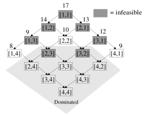
Figure 1: Rank lattice corresponding to the example. The gray nodes are infeasible. The shaded area is the set of nodes dominated by feasible nodes. The number above each node is the value of the node. At the outset, the auctioneer knows the structure of the lattice, but knows neither the shadings nor the values of each node.

Given the rank lattice, we can employ search algorithms to find an optimal allocation. In particular, by starting from the root and searching in best-first order (always expanding the fringe node of highest value), we are guaranteed that the first feasible node that is reached is optimal.

FindOptimal$()$
1	$\ignorespaces\textrm{FRINGE}\leftarrow\{\langle 1,1,\ldots,1\rangle\}$
2	$\mbox{\bf while\ }\textrm{FRINGE}\neq\emptyset$
3	$\ignorespaces r=\mbox{\sc FindBestNode}(\mathop{\textrm{FRINGE}})$
4	$\ignorespaces\mathop{\textrm{FRINGE}}\leftarrow\mathop{\textrm{FRINGE}}-\{r\}$
5	if $r$ is feasible
6	$\ignorespaces\mbox{\bf return\ }r$
7	$\mbox{\bf for\ }\mbox{\bf each\ }r^{\prime}\in\mathop{\textrm{children}}(r)$
8	$\mbox{\bf if\ }r^{\prime}\notin\mathop{\textrm{FRINGE}}$
9	$\ignorespaces\mathop{\textrm{FRINGE}}\leftarrow\mathop{\textrm{FRINGE}}\ \cup\ \{r^{\prime}\}$

Unlike in typical best-first search, algorithm FindOptimal does not necessarily know which node of the fringe has highest value and thus should be expanded next. Determining this often requires more elicitation. We implemented the following algorithm for doing this. It corresponds to an elicitation policy where as long as we cannot prove which node on the fringe is the best, we pick an arbitrary node and elicit just enough information to determine its value.

FindBestNode$(\textrm{FRINGE})$
1	$\ignorespaces S\leftarrow\textrm{FRINGE}$
2	remove from $S$ all $r$ dominated by some $r^{\prime}$ in $S$
3	if all $r\in S$ have the same value
4	$\ignorespaces\mbox{\bf return\ }\mathop{\textrm{arbitrary}}r\in S$
5	choose $r\in S$ whose value we don’t know exactly
6	$\mbox{\bf for\ }\mbox{\bf each\ }\mathop{\textrm{agent $i$}}$
7	if elicitor does not know $b_{i}(r_{i})$
8	ask agent $i$ what bundle it ranks $r_{i}$th
9	if elicitor does not know $v_{i}(b_{i}(r_{i}))$ exactly
10	ask agent $i$ for its valuation on bundle $b_{i}(r_{i})$
11	$\ignorespaces\mbox{\bf goto\ }2$

In some cases, FindBestNode can return a rank vector $r$ although not all bundles $b_{i}(r_{i})$ are known to the elicitor. This can occur, for example, if the known valuations in the rank vector already sum up to a large enough number. In that case, checking the feasibility in step 5 of FindOptimal requires eliciting the unknown bundles $b_{i}(r_{i})$.

5 Experimental setup

While the idea and some algorithms for preference elicitation in combinatorial auctions have been presented previously [4], they have not been validated. To evaluate the usefulness of the idea, we conducted a host of experiments. We present the results in the rest of the paper. Each plot shows how many queries were needed to find an optimal allocation and prove that it is optimal (that no other allocation is better). In each plot, each point represents an average over 10 runs, where each run is on a different problem instance (different draw of valuations for the agents). Each algorithm was tested on the same set of problem instances.

Because the evaluation is based on the amount of information asked rather than real-time, we did not optimize our algorithm implementations for time or space efficiency, but only for elicitation efficiency. Generating all the plots in this paper took two days of computer time on a 1 GHz Pentium III.

Unfortunately, real data for combinatorial auctions are not publicly available. Therefore, as in all of the other academic work on combinatorial auctions so far, we used randomly generated data. We first considered using existing benchmark distributions. However, the existing problem generators output instances with sparse bids, that is, each agent bids on a relatively small number of bundles. This is the case for the CATS suite of economically-motivated random problem instances [12] as well as for the other prior benchmarks [24, 7, 1, 6]. In such cases, the communication is a non-issue, which undermines the purpose of elicitation. In addition, the instances generated by many of the earlier benchmarks do not honor the free disposal constraints (because for an agent, the value of a bundle can be less than that of a sub-bundle).

In many real settings, each bidder has a nonzero valuation for every bundle. For example in spectrum auctions, each bidder has positive value for every bundle because each item is of positive value to every bidder (at least due to renting and reselling possibilities). In other settings, there may exist worthless items for some bidders. Even in such cases, under the free disposal assumption, the bidders have positive valuations for almost all bundles—except bundles that only contain worthless items (because, at worst, they can throw away the extra items in any bundle for free).

To capture these considerations, we developed a new benchmark problem generator. In each problem instance we generate, each bidder has a nonzero valuation for almost every bundle, and all valuations honor free disposal. Specifically, the generator assigns, for each agent in turn, integer valuations using the following routine. We impose an arbitrary maximum bid value $\mathrm{MAXBID}=10^{7}$ in order to avoid integer arithmetic overflow issues, while at the same time allowing a wide range of values to be expressed. Valuations generated with this routine exhibit both complementarity and substitutability.

GenerateBids$(k)$
1	$\ignorespaces G\leftarrow\textrm{new constraint network}$
2	$\ignorespaces S\leftarrow 2^{K}\textrm{\hskip 3.61371pt(the set of all bundles)}$
3	impose free disposal constraints on $G$
4	$\ignorespaces\textit{UB}(K)\leftarrow\mathrm{MAXBID}$
5	$\mbox{\bf while\ }S\neq\emptyset$
6	pick $b$ uniformly at random from $S$
7	$\ignorespaces S\leftarrow S-{b}$
8	pick $v(b)$ uniformly at random from $[\textit{LB}(b),\textit{UB}(b)]$
9	propagate $\textit{LB}(b)=\textit{UB}(b)=v(b)$ through $G$

6 Experiments on rank lattice based elicitation

The first experiment evaluates the efficiency of rank lattice based elicitation, see Figure 2. We plot the number of rank queries made (the number of value queries is never greater because a value query is only ever asked after the corresponding rank query). For comparison, we plot the total number of value queries we could have made: $n(2^{k}-1)$ (that is, for each agent, one query for each of the $2^{k}$ bundles except the empty bundle). This corresponds to full revelation of each agent’s valuation function. Because this number grows exponentially in the number of items $k$, we use a log scale on the vertical axis of the plot that shows performance as a function of the number of items. The other plot has a linear-scale vertical axis because full revelation increases linearly in the number of agents $n$.

Figure 2: Rank lattice based elicitation. Left: 2 agents, varying number of items, log scale. Right: 4 items, varying number of agents, linear scale. All other graphs in the paper also follow this convention.

Define the elicitation ratio to be the number of queries asked divided by the number of queries asked in full revelation. Figure 2 Left shows that as the number of items increases, the elicitation ratio approaches zero, that is, only a vanishingly small fraction of the possible queries are asked.

Figure 2 Right shows that as the number of agents $n$ grows, the advantage from rank lattice based elicitation decreases. This is not as important because even under full revelation, the number of queries increases only linearly. Nevertheless, this behavior might be explained by the observation that while the size of the lattice grows exponentially in $n$, the number of feasible nodes only grows polynomially. Specifically, the total number of rank vectors is $(2^{k})^{n}=2^{nk}$ while the number of feasible rank vectors is $n^{k}$ (each of the $k$ items can independently go to any of the $n$ agents). Therefore, as $n$ increases, this rank lattice based search procedure encounters an increasing fraction of infeasible rank vectors before finally finding an optimal allocation.

A very recent theoretical result shows that the algorithm here is as good as any rank lattice based elicitation algorithm [5]. Specifically, this algorithm is a member of the EBF (efficient best-first) family of algorithms, and the result proves that no algorithm based on the rank lattice can guarantee asking fewer queries than an EBF algorithm over all problem instances (unless it sacrifices economic efficiency).

7 General elicitation framework

Given that no rank lattice based algorithm can do better than the one outlined above, we now move to a more general elicitation framework. As we will show, this allows us to develop algorithms that ask significantly fewer queries.

The framework allows a richer set of query types (to accommodate for different settings where answering some types of queries is easier than answering other types); allows more flexible ordering of the queries at run time; and never considers infeasible solutions. We could implement rank queries in this framework, but did not do so in this work, because rank queries are somewhat unrealistic: to answer them would likely require the bidder to evaluate and sort its entire valuation function.

The general algorithm template is a slightly modified version of that of Conen & Sandholm [4]: Solve$()$ 1 $\ignorespaces C\leftarrow\mbox{\sc InitialCandidates}(n,k)$ 2    $\mbox{\bf while\ }\mbox{\bf not\ }\mbox{\sc Done}(C)$ 3 $\ignorespaces q\leftarrow\mbox{\sc SelectQuery}(C)$ 4 $\ignorespaces\mbox{\sc AskQuery}(q)$ 5 $\ignorespaces C\leftarrow\mbox{\sc Prune}(C)$

Here, $C$ is a set of candidates, where a candidate is a vector $c=\langle c_{1},c_{2},\ldots,c_{n}\rangle$ of bundles where the bundles contain no items in common. Unlike with rank vectors, all candidates are feasible. The value of a candidate is $v(c)=\sum_{i}v_{i}(c_{i})$; $\textit{UB}(c)=\sum_{i}\textit{UB}_{i}(c_{i})$ is an upper bound, and $\textit{LB}(c)=\sum_{i}\textit{LB}_{i}(c_{i})$ a lower bound. A candidate $c$ dominates another candidate $c^{\prime}$ if the elicitor can prove that the value of $c$ is at least as high as that of $c^{\prime}$.

InitialCandidates generates the set of all candidates, which is the set of all $n^{k}$ allocations of the $k$ items to the $n$ agents (some agents might get no items). In our experiments, the candidate set is represented explicitly. To scale the implementation to large $k$ and $n$ would require representing it more intelligently in an implicit way.

Prune removes, one candidate at a time, each candidate that is dominated by a remaining candidate. This may eliminate some optimal allocations, but it will never eliminate all optimal allocations—one will always remain. If strict domination were to be used as the criterion, then Solve would find all optimal allocations, at the cost of requiring more elicitation.

Done returns true if $C$ is a set of candidates, each of which is provably optimal. This is the case either if $C$ has only one element, or if all candidates in $C$ have known value (that is, $\forall c\in C,\textit{UB}(c)=\textit{LB}(c)$). Because the algorithm has just pruned, it knows that if all candidates have known value, then they have equal value.

SelectQuery selects the next query to be asked. This function can be instantiated in different ways to implement different elicitation policies, as we will show.

AskQuery takes a query, asks the corresponding agent for the information, and appropriately updates the constraint network. The details of updating the network are discussed in conjunction with each query type below.

7.1 Value queries

The most basic query asks an agent $i$ to reveal $v_{i}(c_{i})$ exactly. We call such queries value queries. Upon receiving the answer, AskQuery sets $\textit{LB}_{i}(c_{i})=\textit{UB}_{i}(c_{i})=v_{i}(c_{i})$ and propagates the new bounds upstream and downstream through the constraint network as described earlier.

Any policy that asks only value queries relies on there being edges in the constraint network, for instance due to free disposal. Otherwise, it needs to ask every query: any value the elicitor has not asked for might be infinite.

7.1.1 Random elicitation policy

The first policy we investigate simply asks random value queries. In the beginning, we generate the set of all $n(2^{k}-1)$ value queries. Whenever it is time to ask a query, the policy chooses a random query from the set, ignoring those it has already asked or for which the value can already be inferred.

We can actually show that if any policy saves elicitation, then this policy also saves elicitation:

Proposition 1

Let $Q=n(2^{k}-1)$ be the total number of queries, and let $q_{\mathit{min}}$ be the number of queries asked by an optimal elicitation policy. For any given problem instance, the expected number of queries that the random elicitation policy asks is at most $\frac{q_{\mathit{min}}}{q_{\mathit{min}}+1}(Q+1)$.

Proof: Assume pessimistically that a query is either required to prove the optimal allocation or useless. Under this assumption, the analysis reduces to the following problem. We have $r$ red “necessary” balls and $b$ blue “useless” balls in a bag. We then randomly draw one ball at a time without replacement. The question is how many balls we expect to draw before all red balls have been drawn. Let $e(r,b)$ be this number. The base case is $e(0,b)=0$, because there are no red balls to draw. In the general case, we pick one ball from the bag. With probability $r/(r+b)$, it is red, so the bag now has $r-1$ red balls and $b$ blue balls. Similarly, with probability $b/(r+b)$, it is blue, so the bag now has $r$ red balls and $b-1$ blue balls. Therefore, $e(r,b)=1+\frac{r}{r+b}e(r-1,b)+\frac{b}{r+b}e(r,b-1)$. It is easy to verify that $e(r,b)=\frac{r}{r+1}(b+r+1)$ solves this recurrence. In the elicitation setting, $r=q_{\mathit{min}}$ and $r+b=Q$. The result follows.   

The upper bound given in the above proposition only guarantees relatively minor savings in elicitation (especially because $q_{\mathit{min}}$ increases when the number of agents and items increases). This could be due to either the bound being loose, or due to this elicitation policy being poor, or both. The experiment in Figure 3 shows that this elicitation policy is poor—even in the average case. The policy asks almost all of the queries.

Figure 3: Random elicitation policy.

7.1.2 Random allocatable bundle elicitation policy

Essentially, the random elicitation policy asks many queries which, as it turns out, are not useful. We will now present a useful restriction on the set of queries from which the elicitation policy should choose. The key observation is that the elicitor might already know that a bundle is not going to be allocated to a particular bidder—even before the elicitor knows the bidder’s valuation for the bundle. This can occur if the elicitor knows that it cannot obtain enough value from the other bidders for the items not in that bundle. On the other hand, if the elicitor cannot (yet) determine this, then the bundle-agent pair is called an allocatable.

Definition 1

A bundle-agent pair $(b,i)$ is allocatable if there exists a remaining candidate allocation $c\in C$ such that $c_{i}=b$. In some places, the reference to the agent is obvious from the context, so we sometimes talk about allocatable bundles $b$ rather than $(b,i)$.

Now we can refine our random elicitation policy to ask queries on allocatable $(b,i)$ only (and queries that have already been asked or whose answer can be inferred are again never asked).

This restriction is intuitively appealing, and we can characterize cases where it cannot hurt. We define the notation $\langle x,y\rangle$ to mean that revealing the value of a non-allocatable pair $(b,i)$ would raise the lower bound on $x$ allocatable super-bundles of $b$ (that is, there are $x$ allocatable pairs $(b^{\prime},i)$ such that $b^{\prime}\succeq b$), and lower the upper bound on $y$ allocatable sub-bundles of $b$. To affect a lower bound, $v_{i}(b)$ must be strictly greater than the currently-proven lower bound on any of the $x$ super-bundles. Similarly, $v_{i}(b)$ must be strictly less than the currently-proven upper bound on the $y$ sub-bundles.

Given this notation, we can examine the cases where eliciting a non-allocatable $(b,i)$ is no more useful than eliciting some allocatable $(b^{\prime},i)$. Because the elicitor does not know $v_{i}(b)$, it cannot know what case actually applies.

Proposition 2

No matter what value queries the elicitor has asked so far, querying a non-allocatable $(b,i)$ in case $\langle x,y\rangle$ with $x+y<2$ cannot help the unrestricted random elicitation policy ask fewer queries than the restricted random elicitation policy.

Proof: We analyze each case separately.

Case $\langle 0,0\rangle$: In this case, $b$ has no allocatable sub- or super-bundles, so obtaining values for those bundles cannot be useful. So, if $b$ itself is not allocatable, eliciting a value for $b$ cannot be useful. (Here, “useful” means that it helps prove that an allocation is optimal or it helps prove that an allocation is not optimal.)

Cases $\langle 0,1\rangle$ and $\langle 1,0\rangle$: The two cases are symmetric; we assume $\langle 0,1\rangle$ here. Let the single allocatable sub-bundle of $b$ be called $b^{\prime}$. By eliciting $v_{i}(b)$, the upper bound on $v_{i}(b^{\prime})$ will be tightened. However, eliciting $v_{i}(b^{\prime})$ would reveal an upper bound on $b^{\prime}$ that is at least as tight. So eliciting the allocatable bundle $b^{\prime}$ would have been no worse. In fact, it might have been strictly better: with the same number of queries, eliciting $v_{i}(b^{\prime})$ also reveals a lower bound on $b^{\prime}$ and any super-bundle of $b^{\prime}$ (in particular, any allocatable super-bundle).   

While the idea of restricting the queries to allocatable bundles is intuitively appealing and can never hurt in the cases above, there are cases where this restriction forces the elicitor to ask a larger number of queries:

Proposition 3

Querying a non-allocatable $(b,i)$ in case $\langle x,y\rangle$ with $x+y\geq 2$ may help the unrestricted random elicitation policy ask fewer queries than the restricted random elicitation policy.

Proof: Assume there are two bidders. Further assume that given the information elicited previously, there are only three allocations that could be optimal ($|C|=3$). One allocation involves giving bidder 1 the items in bundle $b^{\prime}$, and the other items to bidder 2, and bidder 2 places a value of 50 on those items. Similarly, the second allocation gives bidder 1 the items in bundle $b^{\prime\prime}$, and the other items to bidder 2, who again places a value of 50 on those items. Bundle $b^{\prime}$ is neither a super-bundle nor a sub-bundle of $b^{\prime\prime}$. Given the information elicited so far, the elicitor knows $\textit{UB}_{i}(b^{\prime})=\textit{UB}_{i}(b^{\prime\prime})=100$. A third allocation gives bidder 2 all the items, and bidder 2 places a value of 100 on this outcome; bidder 1 gets no items. Finally, assume the true value agent 1 has on bundle $b$ is 40 ($v_{1}(b)=40$), and that $b$ is not allocatable for agent 1. This means that $(b,1)$ is in case $\langle 0,2\rangle$.

$v_{1}(b^{\prime})=[0,100]$	$v_{2}(K-b^{\prime})=50$	sum: $[0,150]$
$v_{1}(b^{\prime\prime})=[0,100]$	$v_{2}(K-b^{\prime\prime})=50$	sum: $[0,150]$
$v_{1}(\emptyset)=0$	$v_{2}(K)=100$	sum: $100$

Table 1: Example of case $\langle 0,x\rangle$ where revealing a non-allocatable bundle $b$ is better than revealing any allocatable bundle. By eliciting $v_{1}(b)=40$, the elicitor learns that the first two candidate allocations have a value of at most 90, and can therefore eliminate them.

In this situation, by eliciting just $v_{1}(b)$, the elicitor would prove that the third allocation (giving bidder 2 all the items) is optimal. Restricted to revealing allocatable bundles $b^{\prime}$ and $b^{\prime\prime}$ but not $b$, the elicitor will instead need to use two queries instead of just one.   

Proposition 3 does not mean that all cases $\langle x,y\rangle$ with $x+y\geq 2$ are bad. Indeed, it could be that eliciting the non-allocatable $(b,i)$ gives insufficiently tight bounds on the allocatable bundles it affects, and therefore the allocatable bundles need to be elicited anyway. An open problem is whether, in the case of an oracle that chose the best bundle to elicit every time, the bad cases would ever happen.

The case-by-case analysis of Propositions 2 and 3 indicates that restricting the elicitation policy to choosing only allocatable bundles will often help, but may sometimes also cause harm. However, the harm is limited, as we now show.

Proposition 4

Any bad case $\langle x,y\rangle$ with $x+y\geq 2$ causes the random query policy that restricts itself to allocatable queries to ask at most twice as many queries (in expectation) as the unrestricted random policy. This bound is tight.

Proof: Assume that to prove an optimal allocation, it is necessary either to reveal the single non-allocatable bundle, or all of the $x+y$ allocatable bundles. If fewer than all $x+y$ bundles are needed, or if there is more than one subset of the $x+y$ that is sufficient, this only reduces the advantage of being allowed to ask the bad-case query.

In the restricted policy, which cannot ask the bad-case query, the elicitor will ask $x+y$ queries. In the unrestricted policy, the elicitor’s task corresponds to removing balls one at a time from a bag that has 1 red ball and $b=x+y$ blue balls until either the red ball has been removed, or all the blue balls have been removed. Let $e(b)$ be the number of balls we expect to pick until we are done. We pick a red ball with probability $1/(b+1)$ and are done immediately. Otherwise, we pick a blue ball with probability $b/(b+1)$. Therefore, $e(b)=\frac{1}{b+1}+\frac{b}{b+1}(1+e(b-1))$. If only one blue ball is left, whether we pick the red ball or the blue ball, we are done, so $e(1)=1$. It can be verified that $e(b)=\frac{b(3+b)}{2(1+b)}$ solves the recurrence relation. Therefore, the ratio of queries asked in the restricted policy to queries asked in the unrestricted policy is $(x+y)/e(x+y)\leq 2$.   

Summarizing, restricting value elicitation to allocatable bundles either helps, does not hurt, or at worst only causes the elicitor to ask (in expectation) twice as many queries. We ran experiments (Figure 4) to determine whether the restriction helps in practice. The results are clear: at $k=10$, the elicitation ratio is $17\%$. That is, the random elicitation policy restricted to eliciting only allocatable $(b,i)$ avoids the vast majority of the elicitation needed in full revelation or in the unrestricted random elicitation policy. Most importantly, as the number of items increases, the elicitation ratio continues to decrease (unlike with the random elicitation policy without the restriction). Also, unlike with rank lattice based elicitation, as the number of agents increases, the elicitation ratio stays constant or may even decrease.

Figure 4: Random allocatable-only elicitation policy.

This policy is simpler than the value-query policy previously proposed by Conen & Sandholm [4]. That policy counted the number of remaining candidates in which a given bundle $b$ is allocated to agent $i$, and elicited the value of the $(b,i)$ pair with the highest count. We ran the same experiment with that policy. Interestingly, that policy does far less well: depending on the tie-breaking scheme, it asked exactly all the queries (when breaking ties in favor of the smaller bundle, arbitrarily choosing among equal-size bundles), or it converged to about half the queries (when breaking ties in favor of the larger bundle). A randomized tie-breaking scheme did slightly worse than breaking ties in favor of larger bundles.

7.1.3 The grand bundle is (almost) always revealed

Intuitively it is appealing to elicit from every agent the value for the grand bundle because that sets an upper bound on all bundle-agent pairs (via the free disposal assumption). In this section we analyze whether this indeed is a good idea.

Proposition 5

In order to determine the optimal allocation, any elicitation policy must prove an upper bound on $v_{i}(K)$ for every $i$ to which $K$ is not allocated.

Proof: The lower bound on the optimal allocation is finite (say, $L$) because we require each bundle to have non-negative and finite value for every bidder. Therefore, unless the auctioneer provides an upper bound on $v_{i}(K)$, the possibility is open that allocating $K$ to $i$ is worth more than $L$. Because allocating $K$ to $i$ possibly has value greater than implementing the allocation that is, in fact, optimal, the elicitation policy cannot terminate.   

In particular, using value queries only (and with no extra structure beyond free disposal), the only way the auctioneer can establish an upper bound on $v_{i}(K)$ is by eliciting the value.

Theorem 1

Assume there are at least 2 bidders. There is a policy (possibly requiring an oracle for choosing the queries) using value queries that asks $v_{i}(K)$ for every $i$ and that asks the fewest possible questions.

Proof: If the optimal allocation involves allocating items to at least two bidders, then we are not allocating the full bundle to any agent, so by the proposition above, the auctioneer must elicit $v_{i}(K)$ for every $i$.

Otherwise, the optimal allocation involves allocating all items to a single agent $i$. For all $j\neq i$, the proposition applies and therefore the auctioneer must elicit $v_{j}(K)$. What is left to prove is that the auctioneer is at least as well off also eliciting $v_{i}(K)$.

If all other bidders have zero value on all sub-bundles (that is, the full bundle has positive value to them, but anything less has zero value), then the auctioneer need only place a lower bound on $v_{i}(K)$ that is higher than any other bidder’s, which it can do by eliciting $v_{i}(K)$.

If any other bidder $j$ has nonzero value on some bundle $K-b$, the auctioneer needs to prove that $v_{j}(K-b)+v_{i}(b)\leq v_{i}(K)$. In other words, the auctioneer needs to provide a lower bound on $v_{i}(K)$ that is sufficiently greater than the upper bound on $v_{i}(b)$. Using value queries and assuming free disposal, the auctioneer can prove an upper bound on $v_{i}(b)$ by eliciting $b$ or any super-bundle $b^{\prime}$. Similarly, it can prove a lower bound on $K$ by eliciting $K$ or any sub-bundle. However, it cannot prove sufficiently tight bounds to separate the optimal allocation (of $K$ to $i$) from the suboptimal one by eliciting a single bundle: by eliciting a single bundle, it would prove $\textit{UB}_{i}(b)=\textit{LB}_{i}(K)$. Given that it must elicit two bundles, it may as well elicit $v_{i}(K)$ to provide the lower bound on that value.

The argument in the paragraph above generalizes to settings where there are many bidders $j$ who have nonzero value for several bundles $K-b$. The auctioneer must prove a sufficiently tight lower bound on $K$, and sufficiently tight upper bounds on each of the bundle-agent pairs $(b,i)$. Since not all the elicitations that support sufficiently tight upper bounds on $b$’s can also support a sufficiently tight lower bound on $K$, the auctioneer must elicit at least one other bundle to support that lower bound. There may be more than one choice for this; however, one possible choice is simply to elicit $v_{i}(K)$.   

If $n=1$, the statement does not hold because without revealing anything, we already know by free disposal that giving the bidder all of $K$ is an optimal allocation.

7.2 Order queries

In some applications, agents might not know the values of bundles, and might need to expend a lot of effort to determine them [21, 11], but might easily be able to see that one bundle is preferable over another. In such settings, it would be sensible for the elicitor to ask order queries, that is, ask an agent $i$ to order two given bundles $c_{i}$ and $c_{i}^{\prime}$ (to say which of the two it prefers). The agent will answer $c_{i}\succeq c_{i}^{\prime}$ or $c_{i}^{\prime}\succeq c_{i}$ or both. AskQuery will then create new edges in the constraint network to represent these new dominates relations. By asking only order queries, the elicitor cannot compare the valuations of one agent against those of another, so it cannot determine a social welfare maximizing allocation. However, order queries can be helpful when interleaved with other types of queries.

7.3 Using value and order queries

We developed an elicitation policy that uses both value and order queries. It mixes them in a straightforward way, simply alternating between the two, starting with an order query. Whenever an order query is to be asked, the elicitor picks an arbitrary pair $(c,c^{\prime})$ of remaining candidates that cannot be compared due to lack of information, chooses an agent $i$ whose ranking of $c_{i}$ and $c_{i}^{\prime}$ is unknown, and asks that agent to order bundles $c_{i}$ and $c_{i}^{\prime}$. (This is the policy for choosing order queries that was proposed by Conen & Sandholm [4].) Whenever a value query is to be asked, the query is chosen using the policy described in the value query section above.

To evaluate the mixed policy, we need a way of comparing the cost of an order query to the cost of a value query. The plots in this section correspond to a cost model where an order query costs 10% of the cost of a value query.

Figure 5 shows that the amount of elicitation grows linearly with the number of agents. Also, as the number of items increases, the cost of the queries is a vanishing fraction of the cost of full elicitation.

Figure 5: Elicitation using value and order queries.

The policy saves elicitation cost compared to the policy that only uses value queries. For example, at 2 agents and 10 items, its elicitation cost averages 324 while the elicitation cost of the value-only policy averages 361. As the relative cost of an order query is decreases, the benefit of interleaving value queries with order queries increases. Also, if order queries are inexpensive, the policy should probably ask more than one order query per value query.

While this mixed policy appears to provide only a modest benefit over using value queries only, its advantage is that it does not depend as critically on free disposal. Without free disposal, the policy that uses value queries only would have to elicit all values. The order queries in the mixed policy, on the other hand, can create useful edges in the constraint network which the elicitor can use to prune candidates.

7.4 Bound-approximation queries

In many settings, the bidders can roughly estimate valuations easily, but the more accurate the estimate, the more costly it is to determine. In this sense, the bidders determine their valuations using anytime algorithms [11, 10]. For this reason, we introduce a new query type: a bound-approximation query. In such a query, the elicitor asks an agent $i$ to tighten the agent’s upper bound $\textit{UB}_{i}(b)$ (or lower bound $\textit{LB}_{i}(b)$) on the value of a given bundle $b$. This query type leads to more incremental elicitation in that queries are not answered with exact information, and the information is refined incrementally on an as-needed basis.

The elicitor can provide a hint $t$ to the agent as to how much additional time the agent should devote to tightening the bound in the query. Smaller values of the hint $t$ make elicitation more incremental, but cause additional communication overhead and computation by the elicitor. Therefore, the hint can be tailored to the setting, depending on the relative costs of communication, bundle evaluation by the bidders, and computation by the elicitor. The hint could also be adjusted at run-time, but in the experiments below, we use a fixed hint $t=0.2$.

To evaluate this elicitation method, we need a model on how the agents’ computation refines the bounds. We designed the details of our elicitation policy motivated by the following specific scenario, although the elicitation policy can be used generally. Let each agent have two anytime algorithms which it can run to discover its value of any given bundle: one gives a lower bound, the other gives an upper bound. Spending time $d$, $0\leq d\leq 1$ will yield a lower bound $v_{i}(b)\sqrt{d}$ or an upper bound $(2-\sqrt{d})v_{i}(b)$. This means that there are diminishing returns to computation, as is the case with most anytime algorithms. Finally, we assume that the algorithms can be restarted from the best solution found so far with no penalty: having spent $d$ time tightening a bound, we can get the bound we would have gotten spending $d^{\prime}>d$ by only spending an additional time $d^{\prime}-d$.

The model of agents’ computation cost here opens the possibility to cheat in the evaluation of the elicitor. As the model is stated, the elicitor could ask an agent to spend $t$ time each on the upper and lower bound. Based on the answers, the elicitor would know the exact value (it would be in the middle between the lower and upper bound). To check that our results do not inadvertently depend on such specifics of the agents’ computation model, we ran experiments using an asymmetric cost function (linear for lower bounds, square root for upper bounds). This did not appreciably change the results.

Using arbitrarily picked bound-approximation queries as the elicitation policy would work, but the more sophisticated elicitation policy that we developed chooses the query that maximizes the expected benefit. This is the amount by which we expect the upper and lower bounds on bundle-agent pairs to be tightened when we propagate the new bound that the queried agent will return (only counting bundle-agent pairs that are included in the set of remaining candidates). To compute the expected benefit, the elicitor assumes that $v_{i}(b)$ is drawn uniformly at random in $[\textit{LB}_{i}(b),\textit{UB}_{i}(b)]$. To estimate the expected change in bounds, the elicitor samples 10 equally spaced values $\hat{v_{i}}(b)$ in that interval. For each value, the elicitor computes (using the cost model described in the previous paragraph) what bound $z$ it would receive if the agent spent additional time $t$ working on that bound and the true value were $\hat{v_{i}}(b)$. Finally, the elicitor observes by how much the values in the constraint network would change if the elicitor were to propagate $z$ through the network (only bundle-agent pairs that are included in the set of remaining candidates are counted).

We evaluated bound-approximation queries using the elicitation policy and agents’ computation model described above. Figure 6 shows that as the number of items increases, only a vanishingly small fraction of the overall computation cost is actually incurred because the optimal allocation is determined while querying only very approximate valuations on most bundle-agent pairs. The method also maintains its benefit as the number of agents increases.

Figure 6: Elicitation using bound-approximation queries. Because it costs $1$ to get a tight upper or lower bound, it costs $2$ to make both bounds be tight. Thus the worst-case line in these plots is $2n(2^{k}-1)$.

7.4.1 Using bound-approximation and order queries

As in the policy that mixed value and order queries, we can alternate between bound-approximation queries and order queries. Figure 7 presents the results when bound-approximation queries are charged as in the previous section, and order queries are charged $\frac{1}{10}$. As the number of agents increases, only a vanishingly small fraction of the cost of full revelation ends up being paid. The method also maintains its benefit as the number of agents grows. The policy saves elicitation cost compared to the policy that only uses value queries. For example, at 2 agents and 8 items, its elicitation cost averages 172 while the elicitation cost of the policy that only uses bound-approximation queries averages 230. Furthermore, as the relative cost of order queries is lowered, the mixed method becomes increasingly superior to using bound-approximation queries alone.

Figure 7: Elicitation using bound-approximation and order queries. The results are truncated to $k=9$ because a run at $k=10$ took longer than 2 days.

8 Conclusions and future research

In all of the elicitation schemes in this paper (except the unrestricted random one), as the number of items for sale increases, the amount of information elicited is a vanishing fraction of the information collected in traditional “direct revelation mechanisms” where bidders reveal all their valuation information. Each of the elicitation schemes (except the rank lattice based one) also maintains its benefit as the number of agents increases.

While the straightforward policies we analyzed work well, some policies that attempt to be more intelligent actually perform poorly (for example, the value query policy described by Conen & Sandholm [4], and some other policies we tried). These poorly-performing policies have in common that they use a heuristic that maximizes the number of candidates that would be affected by the query. In contrast, the bound-approximation query policy that we introduced benefits from the heuristic of maximizing the change in bounds. Future work includes designing additional useful heuristics for selecting queries.

We showed theoretically that if it is possible to save revelation using an elicitation policy, the simple unrestricted random elicitation policy saves revelation. We also presented theoretical and experimental results that suggest that restricting value elicitation to allocatable bundles is beneficial—which was assumed by Conen & Sandholm [4] but is by no means obvious. For the other elicitation policies, our results were experimental. Future work includes studying their performance theoretically as well.

By using the Clarke tax mechanism [3, 28, 8, 27] to determine the payments that the bidders have to pay, we can ensure that in a Bayes-Nash equilibrium, each agent is motivated to answer the queries truthfully, and is not less happy after the auction than before it [4] (under the usual assumption that the agents have quasilinear preferences). These payments can be computed by determining an optimal allocation $n+1$ times: once overall, and once for each agent removed in turn. Even under the highly pessimistic assumption that answers to queries in one of these problems do not help on the other problems, determining the payments entails only an $n$-fold increase in the number of queries. Given that our results show that we have a significantly better than $n$-fold benefit as the number of items grows, this would not change the fact that only a vanishingly small fraction of queries is asked.

Our bound-approximation queries take the incremental nature of elicitation to a new level. The agents are only asked for rough bounds on valuations first, and more refined approximations are elicited only on an as-needed basis. A related approach would be to propose a bound, and ask whether the agent’s valuation is above or below the bound. This suggest a relationship between preference elicitation and ascending combinatorial auctions where the auction proceeds in rounds, and in each round the bidders react to price feedback by revealing demand (e.g., [17, 29, 2, 15, 18]).

Acknowledgments

The authors thank Maverick Woo for his help on the proofs of Propositions 1 and 4.

References

- [1] Arne Andersson, Mattias Tenhunen, and Fredrik Ygge. Integer programming for combinatorial auction winner determination. In Proceedings of the Fourth International Conference on Multi-Agent Systems (ICMAS), pages 39–46, Boston, MA, 2000.
- [2] Sushil Bikhchandani, Sven de Vries, James Schummer, and Rakesh V. Vohra. Linear programming and Vickrey auctions, 2001.
- [3] E H Clarke. Multipart pricing of public goods. Public Choice, 11:17–33, 1971.
- [4] Wolfram Conen and Tuomas Sandholm. Preference elicitation in combinatorial auctions: Extended abstract. In Proceedings of the ACM Conference on Electronic Commerce (ACM-EC), pages 256–259, Tampa, FL, October 2001. A more detailed description of the algorithmic aspects appeared in the IJCAI-2001 Workshop on Economic Agents, Models, and Mechanisms, pp. 71–80.
- [5] Wolfram Conen and Tuomas Sandholm. Partial-revelation VCG mechanism for combinatorial auctions. In Proceedings of the National Conference on Artificial Intelligence (AAAI), Edmonton, Canada, 2002. To appear.
- [6] Sven de Vries and Rakesh Vohra. Combinatorial auctions: A survey. Draft, August 28th, 2000.
- [7] Yuzo Fujishima, Kevin Leyton-Brown, and Yoav Shoham. Taming the computational complexity of combinatorial auctions: Optimal and approximate approaches. In Proceedings of the Sixteenth International Joint Conference on Artificial Intelligence (IJCAI), pages 548–553, Stockholm, Sweden, August 1999.
- [8] Theodore Groves. Incentives in teams. Econometrica, 41:617–631, 1973.
- [9] Holger Hoos and Craig Boutilier. Bidding languages for combinatorial auctions. In Proceedings of the Seventeenth International Joint Conference on Artificial Intelligence (IJCAI), pages 1211–1217, Seattle, WA, 2001.
- [10] Kate Larson and Tuomas Sandholm. Computationally limited agents in auctions. In AGENTS-01 Workshop of Agents for B2B, pages 27–34, Montreal, Canada, May 2001.
- [11] Kate Larson and Tuomas Sandholm. Costly valuation computation in auctions: Deliberation equilibrium. In Theoretical Aspects of Reasoning about Knowledge (TARK), pages 169–182, Siena, Italy, July 2001.
- [12] Kevin Leyton-Brown, Mark Pearson, and Yoav Shoham. Towards a universal test suite for combinatorial auction algorithms. In Proceedings of the ACM Conference on Electronic Commerce (ACM-EC), pages 66–76, Minneapolis, MN, 2000.
- [13] Noam Nisan. Bidding and allocation in combinatorial auctions. In Proceedings of the ACM Conference on Electronic Commerce (ACM-EC), pages 1–12, Minneapolis, MN, 2000.
- [14] Noam Nisan and Ilya Segal. The communication complexity of efficient allocation problems, 2002. Draft. Second version March 5th.
- [15] David C Parkes. iBundle: An efficient ascending price bundle auction. In Proceedings of the ACM Conference on Electronic Commerce (ACM-EC), pages 148–157, Denver, CO, November 1999.
- [16] David C Parkes. Optimal auction design for agents with hard valuation problems. In Agent-Mediated Electronic Commerce Workshop at the International Joint Conference on Artificial Intelligence, Stockholm, Sweden, 1999.
- [17] David C Parkes and Lyle Ungar. Iterative combinatorial auctions: Theory and practice. In Proceedings of the National Conference on Artificial Intelligence (AAAI), pages 74–81, Austin, TX, August 2000.
- [18] David C Parkes and Lyle Ungar. Preventing strategic manipulation in iterative auctions: Proxy-agents and price-adjustment. In Proceedings of the National Conference on Artificial Intelligence (AAAI), pages 82–89, Austin, TX, August 2000.
- [19] Michael H Rothkopf, Aleksandar Pekeč, and Ronald M Harstad. Computationally manageable combinatorial auctions. Management Science, 44(8):1131–1147, 1998.
- [20] Michael H Rothkopf, Thomas J Teisberg, and Edward P Kahn. Why are Vickrey auctions rare? Journal of Political Economy, 98(1):94–109, 1990.
- [21] Tuomas Sandholm. An implementation of the contract net protocol based on marginal cost calculations. In Proceedings of the National Conference on Artificial Intelligence (AAAI), pages 256–262, Washington, D.C., July 1993.
- [22] Tuomas Sandholm. eMediator: A next generation electronic commerce server. In Proceedings of the Fourth International Conference on Autonomous Agents (AGENTS), pages 73–96, Barcelona, Spain, June 2000. Early version appeared in the AAAI-99 Workshop on AI in Electronic Commerce, Orlando, FL, pp. 46–55, July 1999, and as a Washington University, St. Louis, Dept. of Computer Science technical report WU-CS-99-02, Jan. 1999.
- [23] Tuomas Sandholm. Issues in computational Vickrey auctions. International Journal of Electronic Commerce, 4(3):107–129, 2000. Special Issue on Applying Intelligent Agents for Electronic Commerce. A short, early version appeared at the Second International Conference on Multi–Agent Systems (ICMAS), pages 299–306, 1996.
- [24] Tuomas Sandholm. Algorithm for optimal winner determination in combinatorial auctions. Artificial Intelligence, 135:1–54, January 2002. First appeared as an invited talk at the First International Conference on Information and Computation Economies, Charleston, SC, Oct. 25–28, 1998. Extended version appeared as Washington Univ., Dept. of Computer Science, tech report WUCS-99-01, January 28th, 1999. Conference version appeared at the International Joint Conference on Artificial Intelligence (IJCAI), pp. 542–547, Stockholm, Sweden, 1999.
- [25] Tuomas Sandholm, Subhash Suri, Andrew Gilpin, and David Levine. CABOB: A fast optimal algorithm for combinatorial auctions. In Proceedings of the Seventeenth International Joint Conference on Artificial Intelligence (IJCAI), pages 1102–1108, Seattle, WA, 2001.
- [26] Moshe Tennenholtz. Some tractable combinatorial auctions. In Proceedings of the National Conference on Artificial Intelligence (AAAI), Austin, TX, August 2000.
- [27] Hal Varian. Mechanism design for computerized agents. In Usenix Workshop on Electronic Commerce, New York, July 1995.
- [28] W Vickrey. Counterspeculation, auctions, and competitive sealed tenders. Journal of Finance, 16:8–37, 1961.
- [29] Peter R Wurman and Michael P Wellman. AkBA: A progressive, anonymous-price combinatorial auction. In Proceedings of the ACM Conference on Electronic Commerce (ACM-EC), pages 21–29, Minneapolis, MN, October 2000.