Faster Parametric Shortest Path and
Minimum Balance Algorithms

We use Fibonacci heaps to improve a parametric shortest path algorithm of Karp and Orlin, and we combine our algorithm and the method of Schneider and Schneider’s minimum-balance algorithm to obtain a faster minimum-balance algorithm.

For a graph with $n$ vertices and $m$ edges, our parametric shortest path algorithm and our minimum-balance algorithm both run in $O(nm+n^{2}\log n)$ time, improved from $O(nm\log n)$ for the parametric shortest path algorithm of Karp and Orlin and $O(n^{2}m)$ for the minimum-balance algorithm of Schneider and Schneider.

An important application of the parametric shortest path algorithm is in finding a minimum mean cycle. Experiments on random graphs suggest that the expected time for finding a minimum mean cycle with our algorithm is $O(n\log n+m)$.

1 INTRODUCTION

The body of the paper contains five sections. The first section describes the parametric shortest path problem and an algorithm for solving it that runs in $O(nm+n^{2}\log n)$-time on an $n$-vertex graph with $m$ edges. The algorithm is based on an $O(nm\log n)$-time algorithm of Karp and Orlin [7], modified to take advantage of the Fibonacci heap data structure of Fredman and Tarjan [2]. The second section describes the minimum mean cycle problem and how the parametric shortest path algorithm can be used to solve it.

The third section describes the minimum-balance problem and an algorithm for solving it that runs in $O(nm+n^{2}\log n)$-time. The algorithm combines the method of Schneider and Schneider [11], which yields a straightforward $O(n^{2}m)$-time algorithm for the problem, with the parametric shortest path algorithm.

The fourth section describes the results of implementing the parametric shortest path algorithm for finding a minimum mean cycle and running it on random graphs. The results suggest that the expected time for the parametric shortest path algorithm to find a minimum mean cycle is close to $O(m+n\log n)$, and that even for small graphs the algorithm is faster than the $O(nm)$-time algorithm of Karp [6].

A solution to the parametric shortest path problem is given by a sequence of trees, which our algorithm generates but does not store. The final section discusses how the trees may be implicitly stored so that any tree in the sequence can be generated quickly. Also considered in the final section are generalizations of the problems to which our algorithms still apply.

2 PARAMETRIC SHORTEST PATHS

The parametric shortest path problem is a generalization of the standard single-source shortest path problem in which some of the edge costs have a parameter subtracted from them. An instance of the problem is specified by giving a directed graph $G=(V,E,c)$ with edge costs, a source vertex $s$ with all vertices reachable from $s$, and a subset $E^{\prime}$ of the edges representing those edges whose costs have the parameter subtracted from them. Specifically, a particular value $\lambda$ of the parameter yields the directed graph $G_{\lambda}=(V,E,c-\lambda\delta_{E^{\prime}})$ with edge costs, where $(c-\lambda\delta_{E^{\prime}})(e)=c(e)-\lambda\delta_{E^{\prime}}(e)$, and $\delta_{E^{\prime}}(e)=1$ if $e\in E^{\prime}$ and $0$ otherwise. (We adopt the convention that the parameter is subtracted so that influence of parameterized edges on shortest paths increases with the parameter.)

The problem is to determine a shortest path tree in $G_{\lambda}$ for every $\lambda$ such that shortest paths in $G_{\lambda}$ are well defined. It is well known that shortest paths in $G_{\lambda}$ are well defined if and only if $G_{\lambda}$ contains no negative-cost cycle. Thus the problem is to determine a shortest path tree for each $G_{\lambda}$ such that $\lambda\in[-\infty,\lambda^{*}]$, where $\lambda^{*}$ is as large as possible such that $G_{\lambda^{*}}$ has no negative-cost cycle. If $G_{\lambda}$ has no negative-cost cycle for all $\lambda$, then we take $\lambda^{*}=\infty$. In $G_{\infty}$, we take shortest paths to be those that are shortest in $G$ among those that have the maximum number of parameterized edges. Similarly, if $G_{\lambda}$ has a negative-cost cycle for all $\lambda$, we take $\lambda^{*}=-\infty$, and take shortest paths in $G_{-\infty}$ to be those that are shortest in $G$ among those which have the minimum number of parameterized edges.

A solution to the problem is given by a finite sequence of trees $T_{0},T_{1},\ldots,T_{k}$ and a finite non-decreasing sequence of real numbers $-\infty=\lambda_{0}\leq\lambda_{1}\leq\cdots\leq\lambda_{k+1}=\lambda^{*}$ such that $T_{i}$ is a shortest path tree in $G_{\lambda}$ for all $\lambda$ in $[\lambda_{i},\lambda_{i+1}]$. A solution could also be given by a sequence of trees and strictly increasing real numbers. The algorithm we give may produce sequences with some $\lambda_{i}$ equal to $\lambda_{i+1}$. If the second type of solution is desired, such $\lambda_{i}$ and the corresponding $T_{i}$ can simply be removed from the sequence.

Applications of the parametric shortest path problem include the minimum concave-cost dynamic network flow problem [5], matrix scaling [8, 10], and the minimum mean cycle and minimum balancing problems, discussed below.

2.1 An Inductive Method

A natural method for solving the parametric shortest path problem is to proceed tree by tree. That is, determine $T_{0}$ and then inductively determine successive $\lambda_{i}$ and $T_{i}$. This is the method that we use.

The first tree $T_{0}$ for $\lambda_{0}=-\infty$ can be determined by finding a shortest path tree from $s$ by running a standard $O(nm)$-time single source shortest path algorithm on $G_{\alpha}$, where $\alpha<-\sum_{e\in E}|c(e)|$. For this value of the parameter, paths with fewer parameterized edges always cost less than paths with more, so a shortest path tree in $G_{\alpha}$ is also a shortest path tree in $G_{-\infty}$. The shortest path algorithm that is used must be able to detect the case when a negative-cost cycle exists (shortest paths are not well defined), for this will be the case if $\lambda^{*}=-\infty$.

2.2 Pivot Paths

Next we consider the induction step. Suppose that tree $T$ is a shortest path tree from $s$ in $G_{\lambda}$. Consider increasing the parameter from $\lambda$ until it reaches a value $\lambda^{\prime}$ beyond which $T$ ceases to be a shortest path tree. The reason that $T$ ceases to be a shortest path tree is that some path $p$ not in $T$ from $s$ to some vertex $v$ becomes shorter than its counterpart $t_{v}$ (the path from $s$ to $v$) in $T$. In order for this to happen, $p$ must be equal in cost to $t_{v}$ in $G_{\lambda^{\prime}}$ and have more parameterized edges than does $t_{v}$. We call $\lambda^{\prime}$ the pivot point from $T$, and any such path $p$, a pivot path for $T$.

How can we find a pivot path — a shortest path in $G_{\lambda^{\prime}}$ with more parameterized edges than has the corresponding path in $T$ — without knowing $\lambda^{\prime}$? One way would be to consider each path $p$ from $s$ with more parameterized edges than has its corresponding path in $T$. Of these paths, if we choose one that will first become equal in cost to its corresponding path in $T$ as the parameter is increased, we will have a pivot path.

Once we know a pivot path $p$ for $T$, we can determine the pivot point $\lambda^{\prime}$, because the costs of $p$ and $t_{v}$ can coincide at only one value of the parameter. In $G_{\lambda^{\prime}}$, $p$ and its counterpart $t_{v}$ in $T$ are both shortest paths, and thus they and their corresponding prefixes are all of equal cost. Thus all paths in $T\cup p$ are shortest paths. If we construct the subgraph $T^{\prime}$ by deleting all edges of $T$ that lead into vertices of $p$ and adding the edges of $p$, then, provided $T^{\prime}$ is a tree, it is a shortest path tree in $G_{\lambda^{\prime}}$.

To make sure we are making progress in discovering the subgraph $T^{\prime}$, we will rule out degenerate pivot paths — those with a proper prefix with fewer parameterized edges than has the corresponding path in $T$ or with a zero-cost cycle with no parameterized edges. From any degenerate pivot path, we can construct a nondegenerate pivot path by replacing the offending proper prefix by the corresponding path in $T$ or by deleting the offending cycle. For the rest of the paper when we refer to a pivot path we will mean a nondegenerate pivot path.

This gives us the following algorithm. Determine an initial shortest path tree $T_{0}$ for $G_{-\infty}$. Look for a (nondegenerate) pivot path $p$ for $T_{0}$. If there is none, stop. Otherwise, use this path to determine the pivot point and a subgraph $T^{\prime}$. If $T^{\prime}$ is not a tree, stop. Otherwise, take $T^{\prime}$ to be the next shortest path tree and continue.

If the algorithm stops because there are no pivot paths, then the current shortest path tree will continue to be a shortest path tree indefinitely as the parameter is increased, and $\lambda^{*}=\infty$.

Otherwise, the algorithm may stop because $T^{\prime}$ is not a tree. The subgraph $T^{\prime}$ is formed by replacing the edges in the tree $T$ that lead into the vertices on the pivot path with the pivot path edges. Thus, $T^{\prime}$ can only fail to be a tree if it contains a cycle and can only contain a cycle if the pivot path $p$ contains a cycle. But if $p$, a shortest path, contains a cycle, it must be a zero-cost cycle. Since $p$ is nondegenerate, the cost of the cycle must be decreasing with the parameter. Thus the graph will have a negative-cost cycle for any larger value of the parameter and $\lambda^{*}=\lambda^{\prime}$.

Thus, if the algorithm terminates, it gives a correct sequence of trees and intervals. To bound the number of trees produced by the algorithm, consider the number of parameterized edges on the path into each vertex in $T$ and $T^{\prime}$. By the construction of $T^{\prime}$ and the nondegeneracy of the pivot path, the path in $T^{\prime}$ into a vertex contains at least as many parameterized edges as does the path in $T$. Furthermore, at least one vertex in $T^{\prime}$ has more parameterized edges. Thus, the sum over all vertices of the number of parameterized edges on the path into the vertex in the current tree increases by at least one with each new tree. Since this sum is nonnegative and bounded above by $n^{2}$ (actually $n(n-1)/2$), it follows that the algorithm produces at most $n^{2}$ trees.

2.3 A Faster Implementation

First, we will reduce the number of potential pivot paths that the algorithm checks. Suppose there is a (nondegenerate) pivot path, and let $p$ denote its shortest prefix that is still a pivot path. Let $v$ denote the destination vertex of $p$. Any proper prefix of $p$ is not a pivot path, yet is a shortest path in $G_{\lambda^{\prime}}$ and has at least as many parameterized edges as does the corresponding path in $T$. Thus, each proper prefix of $p$ has the same number of parameterized edges as does its counterpart in $T$, and if we replace any proper prefix of $p$ by its counterpart in $T$, we obtain a pivot path. In particular, if we replace the largest proper prefix of $p$ by its counterpart in $T$, we obtain a pivot path that consists of a path in $T$ followed by an edge (necessarily not in $T$). For each edge $e=(u,v)$, we let $p(e)$ denote the path in $T$ from $s$ to $u$ followed by the edge $e$. Thus, if any pivot path exists, some $p(e)$ is a pivot path. We call any such $p(e)$ a canonical pivot path.

In order to find a canonical pivot path quickly, we will associate with each edge $e=(u,v)$ the value of the parameter, if any, at which the cost of the path $p(e)$ will become equal to the cost of $t_{v}$. Since $t_{v}$ is of cost no more than that of $p(e)$ for the current value of the parameter, this value will exist if and only if $p(e)$ has more parameterized edges than does $t_{v}$. In this case, we call the value the key of the edge. Otherwise, the key of the edge is taken to be infinity. More specifically, let $c(p)$ denote the cost of a path $p$ in $G$ and let $\delta_{E^{\prime}}(p)$ denote the number of parameterized edges on $p$, so that $c(p)-\lambda\delta_{E^{\prime}}(p)$ is the cost of a path $p$ in $G_{\em\lambda^{\prime}}$. Then, the key of $e$ is

$$\frac{c(p(e))-c(t_{v})}{\delta_{E^{\prime}}(p(e))-\delta_{E^{\prime}}(t_{v})}$$

provided $\delta_{E^{\prime}}(p(e))>\delta_{E^{\prime}}(t_{v})$, and infinity otherwise.

Since $p(e)$ is just $t_{u}$ followed by $e$, we can calculate edge keys in constant time if we maintain for each path $t_{w}$ the values $c(t_{w})$ and $\delta_{E^{\prime}}(t_{w})$. When a pivot occurs and the tree changes, we can find (and update) the vertices for which these values change by searching in $T$ from the end of the pivot path. Furthermore, these values only change for a vertex when it acquires a new shortest path, so the time to maintain these values over the course of the algorithm is proportional to the number of shortest path changes over the course of the algorithm, and, thus, at most $n^{2}$.

This gives us an implementation running in $O(n^{2}m)$ time — maintain the tree $T$, maintain the values $c(t_{w})$ and $\delta_{E^{\prime}}(t_{w})$, and perform each of the at most $n^{2}$ pivots by choosing the minimum edge key in $O(m)$ time to define a pivot path.

If we store the edge keys in a standard heap data structure, the time to find each minimum is reduced to $O(\log n)$, so the total time to find minimum keys is reduced to $O(n^{2}\log n)$. The time to maintain the keys increases to $O(\log n)$ per key change, but since the key of an edge is changed only when one of its endpoints acquires a new path, the total number of edge key changes during the course of the algorithm is at most $2nm$. (Recall that each time a vertex acquires a new shortest path, the number of parameterized edges on its current path increases, so that no vertex acquires a new path more than $n-1$ times during the course of the algorithm.) Thus the total time spent maintaining keys is $O(nm\log n)$. This implementation of the algorithm, which is the implementation given by Karp and Orlin [7], therefore runs in time $O(nm\log n)$.

2.4 Vertex Keys

A complete, but different, exposition of the $O(nm\log n)$-time algorithm described above was given by Karp and Orlin in 1981, before the discovery by Fredman and Tarjan of the Fibonacci heap data structure [2] in 1984. The advantage of the F-heap data structure is that the time taken to decrease or insert a key is $O(1)$ in the amortized sense [13]. The time taken to find the minimum key or increase a key is $O(\log n)$ in the amortized sense. Although we can construct graphs yielding $\Theta(nm)$ key increases, so that storing the edge keys in an F-heap does not immediately give a faster algorithm, we can still use an F-heap to our advantage.

To do this, we associate with each vertex $v$ a key that is the minimum of the keys of the edges entering $v$. This is the value of the parameter at which the cost of one of the potential pivot paths $p(e)$ into $v$ will first become equal to the cost of the current path into $v$. With this value we associate the edge $e$.

The minimum vertex key still yields a canonical pivot path. When a pivot occurs, and a vertex acquires a new shortest path, what effect does that have on the vertex keys? Recall that when a vertex acquires a new shortest path, the new path has more parameterized edges. The cost of the new path equals the cost of the old path at the pivot point, but is decreasing faster with the parameter. How the key of a vertex $v$ changes depends on whether the path into $v$ changes and how the potential pivot paths into $v$ change. Suppose the vertex does not acquire a new shortest path and none of the potential pivot paths into it change. In this case, the key remains the same. If the vertex does not acquire a new shortest path but some potential pivot path into it changes, then the cost of the new potential pivot path is decreasing faster than is the cost of the old. In this case, the new path will overtake the current path into $v$ sooner, so if the vertex key changes, it will only decrease.

If a vertex acquires a new shortest path, and none of the potential pivot paths change, then the cost of the new shortest path, which is decreasing faster, will not be overtaken as soon as the old. Thus, in this case, the key will increase. For the remaining case, note that the number of parameterized edges on each new shortest path exceeds the number on the coresponding old path by the same amount. Thus, in this case, the key will stay the same if any of the potential pivot paths that determined the minimum value previously also change, and, otherwise, the key will increase.

To summarize, a vertex key is the minimum of the keys of the edges into the vertex. The algorithm stores with each vertex key the edge whose key determines the value of the vertex key. As before, the algorithm determines a pivot path from the minimum key, computes the new tree $T^{\prime}$, and updates the values $c(t_{w})$ and $\delta_{E^{\prime}}(t_{w})$ for each $w$ that acquires a new shortest path. To maintain the vertex keys, for each vertex that acquires a new shortest path, the algorithm examines the keys of the edges coming into the vertex and takes the new vertex key to be the minimum (possibly increasing the key) and checks the key of each outgoing edge to see if it has decreased below the key of the vertex at the other end, and if it has, it updates that vertex key. It then continues pivoting, as before.

The purpose of this modification is that now the algorithm needs to do fewer increase key operations in the worst case, so that the time taken by the algorithm is reduced by storing the keys in an F-heap. In particular, we will see next that the time taken to maintain keys, which dominates the time taken by the algorithm, is reduced from $O(nm\log n)$ to $O(nm+n^{2}\log n)$.

2.5 Running Time

To bound the time taken by the algorithm, we note that the initialization of the data structures takes $O(m)$-time, plus $O(nm)$-time if a shortest path algorithm needs to be run to determine the initial tree. To bound the remaining time, we will associate each operation involved in updating the data structures with a shortest path change to some vertex and then bound the total number of shortest path changes during the course of the algorithm. We give a slightly more detailed analysis than necessary, which will be useful in Section 5.

Let $m_{w}$ and $j_{w}$ denote the degree of vertex $w$ and the number of shortest path changes (“jumps”) to $w$ in the course of the algorithm, respectively. As noted above, for any graph, $j_{w}\leq n-1$. Once pivoting begins, finding a pivot path takes amortized time $O(\log n)$. At each pivot some vertex changes path, so the time for finding pivot paths is $O(\log n\sum_{w}{j_{w}})$. After a pivot is found, for each vertex that changes path, the shortest path information for the vertex is updated, the edges into and out of the vertex are examined, the vertex key may be increased, and the vertex keys of adjacent vertices may be decreased. Thus, each time $w$ changes path, the amortized time to maintain the data structures is $O(\log n+m_{w})$. [Recall that the amortized times for increase key and decrease key operations in the F-heap are, respectively, $O(\log n)$ and $O(1)$.] Thus, the time taken by the algorithm after initialization is bounded by a constant times

$$\sum_{w}{j_{w}m_{w}}+\log n\sum_{w}{j_{w}}$$

$$\leq n\sum_{w}{m_{w}}+\log n\sum_{w}{j_{w}}$$

$$\leq 2nm+n^{2}\log n.$$ (2)

Thus, the algorithm always runs in time $O(nm+n^{2}\log n)$.

3 THE MINIMUM MEAN CYCLE PROBLEM

The minimum mean cycle problem for a graph with cycles is to find a directed cycle in the graph that minimizes the average cost of the edges on the cycle. The average edge cost of such a cycle is called the minimum cycle mean. Solutions to this problem are needed in a minimum-cost circulation algorithm of Goldberg and Tarjan [3] and in a graph minimum-balancing algorithm of Schneider and Schneider [11]. The problem has been studied by Karp [6], who gave an $O(nm)$-time dynamic programming algorithm, and by Ahuja and Orlin [1], who gave an $O(\sqrt{n}m\log{nC})$-time scaling algorithm. (Here, $C$ is the maximum of the edge costs, which must be integers for the Ahuja-Orlin algorithm to work correctly.)

As Karp and Orlin [7] have observed, the minimum mean cycle problem can be solved using an algorithm for the parametric shortest path problem. Before we discuss how, we introduce the concept of a potential for a graph. Potentials are related to the dual variables arising when path and flow problems are formulated as linear programs. They are also an inherent part of the minimum balance problem that we discuss in the next section.

A potential is an assignment of real-valued weights to the vertices of the graph. Such a potential acts to change the edge costs of the graph, as follows: The cost of an edge $e=(u,v)$ has the weight of $u$ added to it and the weight of $v$ subtracted from it. Thus, potential $\pi:V\rightarrow\Re$ acting on the graph $G=(V,E,c)$ produces the graph $G^{\pi}=(V,E,c^{\pi})$, where $c^{\pi}(e=(u,v))=c(e)+\pi(u)-\pi(v)$. One useful aspect of potentials is that they do not change shortest paths or costs of cycles.

It is well known that for any graph with no negative-cost cycle, there is a potential for which the resulting graph has all nonnegative edge costs. Specifically, we fix a source vertex $s$ in the graph $G$ from which all vertices are reachable. (If there is no such vertex in the original graph, we introduce an artificial source vertex with zero-cost edges to all other vertices. The minimum mean cycle is unchanged by this alteration.) Let $\pi(v)$ be the cost of the shortest path from $s$ to $v$. Then, the well-known inequality $\pi(v)\leq\pi(u)+c(e)$ holds for every edge $e=(u,v)$. The cost of edge $e$ in $G^{\pi}$ is therefore nonnegative. Furthermore, if $e$ lies on a shortest path, or on a zero-cost cycle, then equality holds in the above relation, so the transformed edge cost is zero. We call $\pi$ a shortest path potential for $G$.

Using the notation of Section 2, with $E=E^{\prime}$, let $G_{\lambda}$ denote the graph $G$ with $\lambda$ subtracted from all edge costs, and let $\lambda^{*}$ denote the largest $\lambda$ such that shortest paths in $G_{\lambda}$ are well defined. As shown earlier, if $\lambda^{*}\neq\infty$, then $G_{\lambda^{*}}$ has a zero-cost cycle, but no negative-cost cycle. It follows that if we apply the shortest path potential $\pi$ for $G_{\lambda^{*}}$ to $G_{\lambda^{*}}$, we obtain a graph with a zero-cost cycle and nonnegative edge costs. If we then add $\lambda^{*}$ to all edge costs, we obtain the graph $G^{\pi}$. It follows that $G^{\pi}$ has a cycle $C$ with each edge of cost $\lambda^{*}$ and that no edge in $G^{\pi}$ has cost less than $\lambda^{*}$. Thus, $C$ is a minimum mean cycle of mean cost $\lambda^{*}$ in $G^{\pi}$. Since potentials do not change cycle costs, $C$ is also a minimum mean cycle in $G$ and the minimum cycle mean in $G$ is $\lambda^{*}$.

Thus, to solve the minimum mean cycle problem, it suffices to obtain a shortest path potential for $G_{\lambda^{*}}$. Such a potential is easily obtainable from the last shortest path tree produced by the parametric shortest path algorithm run on $G$ with all edges parameterized. In this case, the algorithm stops because it discovers a zero-cost cycle in $G_{\lambda^{*}}$, which, in turn, is a minimum mean cycle in $G$. Thus, the minimum mean cycle problem is easily reduced to the parametric shortest path problem.

As a side note, the introduction of an artificial source vertex with zero-cost edges into all the other vertices is useful even if an original source vertex is available. An initial shortest path tree from the artificial source vertex is given by the zero-cost edges, so there is no need to solve an arbitrary single-source shortest path problem. This variant corresponds to the sourceless parameterized shortest path problem, where shortest paths independent of source into each node are computed rather than shortest paths from a particular source. This variation also applies to Karp’s minimum mean cycle algorithm [6] and simplifies it by removing an initial strongly connected components computation. In practice, however, partitioning the graph into strongly connected components might reduce the solution time.

4 THE MINIMUM BALANCE PROBLEM

We say that a subset of the vertices of $G$ is minimum-balanced if the minimum cost among edges entering the subset is the same as is the minimum cost among edges leaving the subset. The minimum-balance problem for a strongly connected graph $G=(V,E,c)$ is to determine a potential $\pi$ such that, in $G^{\pi}$, each subset of the vertices other than $E$ or $\emptyset$ is minimum-balanced. Such a potential is said to minimum-balance $G$. Schneider and Schneider introduced an equivalent problem [11] in connection with matrix balancing, and they gave an $O(n^{2}m)$-time algorithm. Our algorithm, which runs in time $O(nm+n^{2}\log n)$, can be viewed as a faster implementation of Schneider and Schneider’s algorithm.

To solve the minimum balance problem, note that finding a shortest path potential $\pi$ for $G_{\lambda^{*}}$ and a minimum mean cycle $C$ is a step toward minimum-balancing the graph. In $G^{\pi}$, each subset of vertices that $C$ enters and leaves has edges entering and leaving of cost exactly $\lambda^{*}$, and no entering or leaving edge has cost less than $\lambda^{*}$. Consider contracting $C$ to a single new vertex $v$ in $G^{\pi}$, deleting self-loops but retaining multiple edges, to obtain the graph $H$. Let $\beta$ be a potential that minimum-balances $H$. If $H$ has only one vertex, $\beta$ can be taken to be any function; otherwise it can be obtained recursively. The edges of $H^{\beta}$ are all of cost no less then the minimum cycle mean of $H$, which is, in turn, no less than $\lambda^{*}$, the minimum cycle mean of $G$.

To complete the minimum-balancing, we can essentially just add the potentials $\pi$ and $\beta$. Consider extending the potential $\beta$ for $H$ to the potential $\alpha$ for $G^{\pi}$ defined by

$$\alpha(w)=\cases{\beta(v)&$w$ on $C$;\cr\beta(w)&otherwise.\cr}$$

The effect of $\alpha$ on $G^{\pi}$ is as follows. Each edge in $G^{\pi}$ that corresponds to an edge in $H$ becomes of cost equal to the cost of the corresponding edge in $H^{\beta}$. The other edges, joining vertices on the cycle $C$, remain unchanged in cost. Thus, if a subset of the vertices is entered and left by $C$, it is entered and left by edges of cost $\lambda^{*}$, which are minimum. Otherwise, the edges entering and leaving the subset correspond to the edges entering and leaving the corresponding subset of the vertices of $H$, and so the subset is correspondingly minimum-balanced. Thus, the potential $\pi+\alpha$ minimum-balances $G$.

In summary, the minimum-balancing algorithm repeatedly finds and contracts a minimum mean cycle until the graph contains only one vertex. Each time the cycle is contracted, a shortest path potential is computed for the current graph. The minimum-balancing potential is computed by adding together the shortest path potentials, appropriately extended.

At this point we have reduced the minimum-balance problem to a series of at most $n$ problems involving finding minimum mean cycles and shortest path potentials. Schneider and Schneider, who gave the above method in [11], also noted that Karp’s $O(nm)$-time algorithm for finding minimum mean cycles can be extended to yield shortest path potentials, thus obtaining an $O(n^{2}m)$-time algorithm.

4.1 A Hybrid Algorithm

The successive graphs computed by the above method are closely related. By modifying the parametric path algorithm to contract the minimum mean cycle it discovers and continue, we obtain a faster algorithm.

Suppose that we run the parametric shortest path algorithm on $G$ with an arbitrary source $s$ and $E=E^{\prime}$. Since $G$ is strongly connected, the algorithm will terminate, having produced $\lambda^{*}$ and a tree $T_{k}$ that is a shortest path tree in $G_{\lambda^{*}}$. This is sufficient to obtain a shortest path potential for $G_{\lambda^{*}}$, as required by the first iteration of the minimum-balance algorithm.

The minimum-balance algorithm would next adjust the edge costs of $G$ by applying the shortest path potential $\pi$, contract the resulting graph around the discovered minimum mean cycle, and continue. Consider what happens if instead of stopping the parametric shortest path algorithm at this point we try to continue it through the adjustment and contraction.

First, to what extent can we maintain the shortest path tree? We have a tree $T$ that is a shortest path tree in $G_{\lambda^{*}}$. Since potentials preserve shortest paths, $T$ is also a shortest path tree in $G^{\prime}=G_{\lambda^{*}}^{\pi}$. We would like a shortest path tree in $G^{\prime}/C$, $G^{\prime}$ contracted around $C$. By properties of the shortest path potential, we know that edge costs in $G^{\prime}$ are nonnegative and that edges on $C$ or $T$ are of zero cost in $G^{\prime}$. It follows that $T/C$, the tree $T$ contracted around the cycle $C$, has all zero-cost edges in $G^{\prime}/C$. Since $C$ consists of a single edge not in $T$ together with a path in $T$, $T/C$ is a tree in $G^{\prime}/C$. Thus, $T/C$ is a shortest path tree in $G^{\prime}/C$.

Once the shortest path tree $T/C$ is constructed, we can completely recompute the secondary data structures, including $c(t_{w})$ and $\pi_{E^{\prime}}(t_{w})$ for each vertex $w$, the F-heap of vertex keys, and the mapping of which edges have determined which vertex keys, in $O(m)$-time. We are then ready to proceed with the inductive step of the parametric shortest path algorithm, modifying the tree pivot by pivot until the next minimum mean cycle is found.

4.2 Termination and Running Time

The algorithm continues pivoting and contracting, calculating the requisite shortest path potentials at each contraction, until the graph contains only a single vertex. Note that the initial graph and thus all subsequent graphs are strongly connected. Thus, every graph with at least two vertices will have a cycle with a parameterized edge, and so the only way a sequence of pivots can stop is by discovery of a minimum mean cycle.

Since at most $n$ contractions can take place, the time spent by the algorithm performing contractions and reinitializing data structures following a contraction is $O(mn)$. The remaining time is spent pivoting from one tree to the next between contractions. The analysis of the parametric path algorithm bounding the number of pivots and the time spent maintaining the data structures after each pivot in terms of the number of path changes continues to apply here. Each pivot still results in some vertex acquiring a new path, and each operation maintaining the data structures is associated with a path change for some vertex. To obtain the same worst-case bound (2), it suffices to note that the number of shortest path changes during the course of the algorithm is still bounded by $n$ per vertex.

Consider, as the minimum-balance algorithm proceeds, the number of vertices in the graph minus the number of parameterized edges on the shortest path to a vertex $w$. Every time the path changes as the result of a pivot, this quantity decreases, and contraction does not increase it. Furthermore, the quantity initially is at most $n$ and on termination is nonnegative. Thus, it is decreased at most $n$ times, and the number of path changes associated with $w$ is at most $n$.

5 EXPECTED RUNNING TIMES

Although there are graphs for which the worst-case bounds for the parametric shortest path and minimum-balance algorithms are tight, one might suspect that for many, if not most, graphs the bounds are not tight. In the case of the minimum balance algorithm, it may be that, for most graphs, most vertices do not acquire $\Omega(n)$ new shortest paths throughout the course of the algorithm, either because when a vertex acquires a new shortest path that path tends to be substantially longer than the old one, or because the contracted cycles tend to be larger than constant size. Since the work done in the parametric shortest path algorithm is essentially the work done in the minimum balance algorithm before the first contraction, one might expect that the work done by the parametric shortest path algorithm would be even less.

To explore this, consider the behavior of the parametric path algorithm as used for finding a minimum mean cycle on random directed graphs. We can rewrite the bound (2.5) as follows:

$$\sum_{w}{j_{w}m_{w}}+\log n\sum_{w}{j_{w}}$$ (3)

$$\leq \max_{w}{m_{w}}\sum_{w}{j_{w}}+\log n\sum_{w}{j_{w}}$$

$$= \sum_{w}{j_{w}}\left(\max_{w}{m_{w}}+\log n\right).$$

With high probability, the maximum degree of a random directed graph is $O(m/n+\log n)$, so that it remains only to estimate the number of path changes when the algorithm is run on random directed graphs.

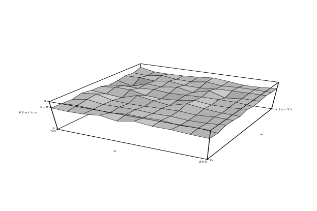
Figure 1: Average number of shortest path changes per vertex when finding a min. mean cycle.

To do this, we ran the sourceless variant of the algorithm on random directed graphs of $n$ nodes and $m$ edges with each of the $n(n-1)$ edges equally likely to be present. For each $n$ and $m$, we took $n/2$ or fifty trials, whichever was larger, and averaged the number of path changes in each trial. Figure 1 shows the average number of path changes per vertex for the parametric path algorithm for finding a minimum mean cycle.

The results suggest that the expected number of path changes for the parametric path algorithm is $O(n)$. If this is true, then the parametric path algorithm yields a minimum mean cycle algorithm with worst case time $O(nm+n^{2}\log n)$ and expected time $O(m+n\log n)$.

We make this argument precise in the following lemma and corollary.

Lemma 1

Given a random directed graph with $n$ nodes and $m$ edges, the probability that some vertex is of degree higher than $8m/n+2\log n$ is less than $2/n$.

Proof. If $8m/n\geq 2(n-1)$ or $n\leq 8$, then clearly the lemma holds. Assume that $m<\frac{1}{4}n(n-1)$ and $n>8$. The number of graphs with $n$ nodes and $m$ edges with a given vertex of degree $d$ is

$$g_{d} = {2(n-1)\choose d}{n(n-1)-2(n-1)\choose m-d}$$

$$= g_{d-1}\frac{(2(n-1)-d+1)(m-d+1)}{d\left(n(n-1)-2(n-1)-(m-d)\right)}$$

$$\leq g_{d-1}\frac{2(n-1)m}{d((n-2)(n-1)-(m-d))}$$

$$\leq g_{d-1}\frac{2(n-1)m}{d((n-2)(n-1)-\frac{1}{4}n(n-1))}$$

$$= g_{d-1}\frac{8m}{d(3n-8)}$$

$$\leq g_{d-1}\frac{4m}{dn}.$$

Thus, letting $D=\left\lceil 8m/n\right\rceil$, for $d>D$, $g_{d}\leq\frac{1}{2}g_{d-1}\leq g_{D}2^{-(d-D)}$. Therefore. the number of graphs with a given vertex of degree greater than or equal to $D+2\log n$ is bounded by

$$\sum_{d\geq D+2\log n}g_{D}2^{-(d-D)}=g_{D}\sum_{i\geq 2\log n}2^{-i}\leq 2g_{D}n^{-2}.$$

Thus the probability that a given vertex is of degree $D+2\log n$ or more is less than $2/n^{2}$. It follows that the the probability that some vertex is this degree or higher is less than $2/n$.  

Corollary 1

If the expected number of path changes is $O(n)$, then the expected running time of the algorithm is $O(m+n\log n)$.

Proof. Let $R$ be the running time of the algorithm on a random graph, let $B$ be the quantity $\sum_{w}{j_{w}}\left(\max_{w}{m_{w}}+\log n\right)$, let $D$ be the event that all vertices of the graph have degree less than $8m/n+2\log n$, and let $J$ be the number of path changes. Then, bounds (2) and (3) and lemma 1 give

$$E(R) \leq E(B)$$

$$= \Pr[D]E(B|D)+\Pr\left[\bar{D}\right]E(B|\bar{D})$$

$$\leq E(J\times\left(8\frac{m}{n}+3\log n\right)|D)$$

$$\ +\frac{2}{n}O(nm+n^{2}\log n)$$

$$= O(m+n\log n)\left(\frac{E(J|D)}{n}+1\right)$$

$$\leq O(m+n\log n)\left(\frac{E(J)}{\Pr[D]n}+1\right)$$

$$= O(m+n\log n).$$

 

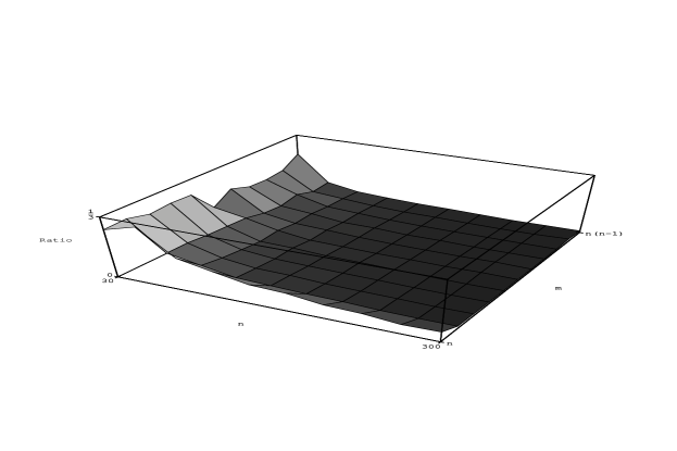
Figure 2: Ratio of average time to average time for Karp’s algorithm.

Figure 2 shows the ratio of the average time for our minimum mean cycle algorithm to the average time of Karp’s $O(nm)$-time minimum mean cycle algorithm, which runs in time $\Theta(nm)$ for all graphs.

Although we did not implement the scaling minimum mean cycle algorithm of Ahuja and Orlin [1], experience with a related algorithm suggests that even if the scaling algorithm runs in expected time $O(n\log n+m)$ for some reasonable distribution of graphs, the constants involved would be larger than those observed for our algorithm [9].

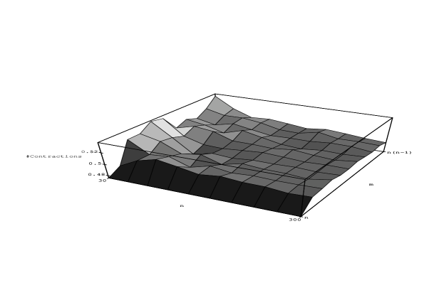
Figure 3: Average number of contractions per vertex.

We also tested the minimum balance algorithm. As Figure 3 shows, it appears that the number of contractions for a nonsparse random graph is about $n/2$. In the algorithm as described, the contraction step, which takes $O(m)$-time per contraction, appears to be the bottleneck, giving a running time of $\Theta(nm)$. The total time for contraction can be reduced to $O(J+n\log n)$, where $J$ is the number of shortest path changes, by using a variant of the union-find data structure of Tarjan [12]. The time for adding the partial potentials is similarly reduced, so this modification should remove the bottleneck. We have not estimated the expected running time of the modified algorithm.

6 FINAL REMARKS

One question not addressed by our parametric path algorithm is the form in which the solution is produced. Recording the sequence of trees explicitly would take space and time $\Theta(n^{3})$ in the worst case of $\Theta(n^{2})$ trees, and recovering a tree for a particular value of the parameter would require locating the value in the sequence of intervals, which can be done easily in $\log n$ time. Alternatively, we can store for each vertex the values of the parameter at which the parent changes and which vertex becomes the parent at each change. Then, in the worst case, the space is $O(n^{2})$ and any tree can be recovered in $O(n\log n)$-time by searching for the parent of each node individually with a binary search. For most graphs, the number of times each vertex changes parent is probably constant, so this is probably an even better solution in practice.

On a different note, a number of generalizations of our algorithms are possible. The parametric path algorithm can be generalized to handle the case in which the edge costs are more general functions of the parameter. In particular, if the edge costs are concave functions of the parameter with derivative in the set $\{-K,\ldots,-1,0\}$, then essentially the same algorithm works, provided that the functions are stored so that for each function we can tell for successive values of the parameter what the current value and derivative are and when the next decrease in derivative will occur. For instance, if we allow the initial graph to contain multiedges, and each multiedge is given as a list of edges with cost functions of constant derivative in $\{-K,\ldots,1,0\}$, in order of decreasing derivative, then pivots still occur when the shortest path into a vertex changes and each such change decreases the derivative of the cost of the path into the vertex. Essentially the same analysis applies to show that the number of path changes to each vertex is in this case at most $Kn$ and the algorithm produces at most $Kn^{2}$ trees in time $O(Knm+Kn^{2}\log n)$.

Surprisingly, the parametric path algorithm can also be generalized to allow concave edge cost functions with positive derivative. If the functions are concave functions of the parameter with derivative in the range $[-K,..,K]$, then the same argument shows that the same type of transition from one shortest path tree to the next occurs. In this case, finding an initial shortest path tree is more difficult, however, because an initial value of the parameter for which shortest paths are well defined is not so easy to come by.

If all edge cost functions are nonnegative at some point (say zero), then we can start by finding a shortest path tree in $G_{0}$ and proceed by increasing the parameter, generating trees in sequence as before, until some cycle becomes of zero cost. Then, we can return to $G_{0}$ and proceed by decreasing the value of the parameter to generate the initial part of the sequence of trees in reverse. We leave open the problem of finding an initial value of the parameter in the general case.

The minimum average weighted length cycle problem [4] is a generalization of the minimum mean cycle problem in which each edge of the graph has a (positive) weight as well as a cost. The problem is to find the cycle that minimizes the ratio of the sum of the costs of the edges on the cycle to the sum of weights of the edges on the cycle. This problem can be reduced to the generalized parametric shortest path problem described above, just as the minimum mean cycle problem can be reduced to the parametric shortest path problem, by taking the cost function of an edge to be the parameter times the weight minus the cost.

We also might consider generalizing the minimum-balance problem by allowing the algorithm to proceed with more general parameterizations. The analysis of the running time still holds, but in this case we know of no natural interpretation of the problem that the algorithm is solving.

Received January, 1990

Accepted April, 1990

References

- [1] R. K. Ahuja and J. B. Orlin. New scaling algorithms for assignment and minimum cycle mean problems. Sloan Working Paper 2019-88, Sloan School of Management, M.I.T., 1988.
- [2] M. L. Fredman and R. E. Tarjan. Fibonacci heaps and their uses in improved network optimization algorithms. J. Assoc. Comput. Mach., 34:596–615, 1987.
- [3] A. V. Goldberg and R. E. Tarjan. Finding minimum-cost circulations by canceling negative cycles. J. ACM, 36:873–886, 1989.
- [4] M. Gondran and M. Minoux. Graphs and Algorithms. Wiley, 1984.
- [5] S. C. Graves and J. B. Orlin. A minimum concave cost dynamic network flow problem, with an application to lot sizing. Networks, 15:59–71, 1985.
- [6] R. M. Karp. A characterization of the minimum cycle mean in a digraph. Discrete Math, 23:309–311, 1978.
- [7] R. M. Karp and J. B. Orlin. Parametric shortest path algorithms with an application to cyclic staffing. Discrete Applied Mathematics, 3:37–45, 1981.
- [8] J. B. Orlin and U. G. Rothblum. Computing optimal scalings by parametric network algorithms. Mathematical Programming, 32:1–10, 1985.
- [9] N. Schlenker. Personal communication. Dept. of Computer Science, Princeton University, Princeton, NJ, 1989.
- [10] H. Schneider and M. H. Schneider. Towers and cycle covers for max-balanced graphs. Unpublished manuscript, 1989.
- [11] H. Schneider and M. H. Schneider. Max-balancing weighted directed graphs and matrix scaling. Mathematics of Operations Research, February 1990.
- [12] R. E. Tarjan. Applications of path compression on balanced trees. J. ACM, 26:690–715, 1979.
- [13] R. E. Tarjan. Amortized computational complexity. SIAM J. Alg. Disc. Math., 6:306–318, 1985.