Preliminary version; to appear in Natural Language Engineering, 2003

Mostly-Unsupervised Statistical Segmentation of Japanese Kanji Sequences

Abstract

Given the lack of word delimiters in written Japanese, word segmentation is generally considered a crucial first step in processing Japanese texts. Typical Japanese segmentation algorithms rely either on a lexicon and syntactic analysis or on pre-segmented data; but these are labor-intensive, and the lexico-syntactic techniques are vulnerable to the unknown word problem. In contrast, we introduce a novel, more robust statistical method utilizing unsegmented training data. Despite its simplicity, the algorithm yields performance on long kanji sequences comparable to and sometimes surpassing that of state-of-the-art morphological analyzers over a variety of error metrics. The algorithm also outperforms another mostly-unsupervised statistical algorithm previously proposed for Chinese.

Additionally, we present a two-level annotation scheme for Japanese to incorporate multiple segmentation granularities, and introduce two novel evaluation metrics, both based on the notion of a compatible bracket, that can account for multiple granularities simultaneously.

1 Introduction

Because Japanese is written without delimiters between words (the analogous situation in English would be if words were written without spaces between them), accurate word segmentation to recover the lexical items is a key first step in Japanese text processing. Furthermore, word segmentation can also be used as a more directly enabling technology in applications such as extracting new technical terms, indexing documents for information retrieval, and correcting optical character recognition (OCR) errors [Wu and Tseng,1993, Nagao and Mori,1994, Nagata,1996a, Nagata,1996b, Sproat et al.,1996, Fung,1998].

Typically, Japanese word segmentation is performed by morphological analysis based on lexical and syntactic knowledge. However, character sequences consisting solely of kanji (Chinese-derived characters, as opposed to hiragana or katakana, the other two types of Japanese characters) pose a major challenge to morphologically-based segmenters for several reasons.

First and most importantly, lexico-syntactic morphological analyzers are vulnerable to the unknown word problem, where terms from the domain at hand are not in the lexicon; hence, these analyzers are not robust across different domains, unless effort is invested to modify their databases accordingly. The problem with kanji sequences is that they often contain domain terms and proper nouns, which are likely to be absent from general lexicons: Fung [Fung,1998] notes that 50-85% of the terms in various technical dictionaries are composed at least partly of kanji. Domain-dependent terms are quite important for information retrieval, information extraction, and text summarization, among other applications, so the development of segmentation algorithms that can efficiently adapt to different domains has the potential to make substantial impact.

Another reason that kanji sequences are particularly challenging for morphological analyzers is that they often consist of compound nouns, so syntactic constraints are not applicable. For instance, the sequence , whose proper segmentation is (president $|$ both-of-them $|$ business $|$ general manager, i.e., a president as well as a general manager of business), could be incorrectly segmented as (president $|$ subsidiary business $|$ (the name) Tsutomu $|$ general manager); since both alternatives are four-noun sequences, they cannot be distinguished by part-of-speech information alone.

An additional reason that accuracy on kanji sequences is an important aspect of the total segmentation process is that they comprise a significant portion of Japanese text, as shown in Figure 1.

Sequence length	# of characters	% of corpus
1 - 3 kanji	20,405,486	25.6
4 - 6 kanji	12,743,177	16.1
more than 6 kanji	3,966,408	5.1
Total	37,115,071	46.8

Figure 1: Kanji statistics from 1993 Japanese newswire (NIKKEI). The sequence length categories are disjoint; to take an analogous example from English: “theQUICKbrownFOX” has three lower-case characters in sequences of length 1-3 and five lower-case characters in sequences of length 4-6.

Since sequences of more than 3 kanji generally consist of more than one word, at least 21.2% of 1993 Nikkei newswire consists of kanji sequences requiring segmentation; and long sequences are the hardest to segment [Takeda and Fujisaki,1987].

As an alternative to lexico-syntactic and supervised approaches, we propose a simple, efficient segmentation method, the tango algorithm, which learns mostly from very large amounts of unsegmented training data, thus avoiding the costs of encoding lexical or syntactic knowledge or hand-segmenting large amounts of training data. Some key advantages of tango are:

• A very small number of pre-segmented training examples (as few as 5 in our experiments) are needed for good performance.

• For long kanji strings, the method produces results rivalling those produced by Juman 3.61 [Kurohashi and Nagao,1999] and Chasen 1.0 [Matsumoto et al.,1997], two morphological analyzers in widespread use. For instance, we achieve on average 5% higher word precision and 6% better morpheme recall.

• No domain-specific or even Japanese-specific rules are employed, enhancing portability to other tasks and applications.

We stress that we explicitly focus on long kanji sequences, not only because they are important, but precisely because traditional knowledge-based techniques are expected to do poorly on them. We view our mostly-unsupervised algorithm as complementing lexico-syntactic techniques, and envision in the future a hybrid system in which our method would be applied to long kanji sequences and morphological analyzers would be applied to other sequences for which they are more suitable, so that the strengths of both types of methods can be integrated effectively.

1.1 Paper organization

This paper is organized as follows. Section 2 describes our mostly-unsupervised, knowledge-lean algorithm. Section 3 describes the morphological analyzers Juman and Chasen; comparison against these methods, which rely on large lexicons and syntactic information, forms the primary focus of our experiments.

In Section 4, we give the details of our experimental framework, including the evaluation metrics we introduced. Section 5 reports the results of our experiments. In particular, we see in Section 5.1 that the performance of our statistics-based algorithm rivals that of Juman and Chasen. In order to demonstrate the usefulness of the particular simple statistics we used, in Section 5.2 we show that our algorithm substantially outperforms a method based on mutual information and t-score, sophisticated statistical functions commonly used in corpus-based natural language processing.

We discuss related work in section 6, and conclude in section 7.

2 The TANGO Algorithm

Our algorithm, tango (Threshold And maximum for N-Grams that Overlap), employs character $n$-gram counts drawn from an unsegmented corpus to make segmentation decisions. We start by illustrating the underlying motivations, using the example situation depicted in Figure 2: “A B C D W X Y Z” represents a sequence of eight kanji characters, and the goal is to determine whether there should be a word boundary between D and W.

The main idea is to check whether $n$-grams that are adjacent to the proposed boundary, such as the 4-grams $s_{L}=$“A B C D” and $s_{R}=$“W X Y Z”, tend to be more frequent than $n$-grams that straddle it, such as the 4-gram $t_{1}=$ “B C D W”. If so, we have evidence of a word boundary between D and W, since there seems to be relatively little cohesion between the characters on opposite sides of this gap.

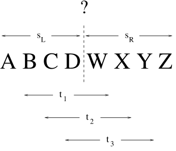
Figure 2: Collecting 4-gram evidence for a word boundary – are the non-straddling $n$-grams $s_{L}$ and $s_{R}$ more frequent than the straddling $n$-grams $t_{1},t_{2},$ and $t_{3}$?

The $n$-gram orders used as evidence in the segmentation decision are specified by the set $N$. For instance, our example in Figure 2 shows a situation where $N=\mbox{$\{4\}$}$, indicating that only 4-grams are to be used. We thus pose the six questions of the form, “Is $\#(s_{d})>\#(t_{j})$?”, where $\#(x)$ denotes the number of occurrences of $x$ in the (unsegmented) training corpus, $d\in\mbox{$\{L,R\}$}$, and $j\in\mbox{$\{1,2,3\}$}$. If $N=\mbox{$\{2,4\}$}$, then two more questions (Is “$\#(\mbox{C D})>\#(\mbox{D W})$?” and “Is $\#(\mbox{W X})>\#(\mbox{D W})$?”) are used as well. Each affirmative answer makes it more reasonable to place a segment boundary at the location under consideration.

More formally, fix a location $k$ and an $n$-gram order $n$, and let $s^{n}_{L}$ and $s^{n}_{R}$ be the non-straddling $n$-grams just to the left and right of it, respectively. For $j\in\mbox{$\{1,2,\ldots,n-1\}$}$, let $t^{n}_{j}$ be the straddling $n$-gram with $j$ characters to the right of location $k$. We define $I_{>}(y,z)$ to be the indicator function that is 1 when $y>z$, and 0 otherwise — this function formalizes the notion of “question” introduced above.

tango works as follows. It first calculates the fraction of affirmative answers separately for each $n$-gram order $n$ in $N$, thus yielding a “vote” for that order $n$:

$$v_{n}(k)=\frac{1}{2(n-1)}\sum_{d\in\mbox{$\{L,R\}$}}\sum_{j=1}^{n-1}I_{>}(\#(s^{n}_{d}),\#(t^{n}_{j})).$$

Note that in locations near the beginning or end of a sequence, not all the $n$-grams may exist (e.g., in Figure 2, there is no non-straddling 4-gram to the left of the A-B gap), in which case we only rely on comparisons between the existing relevant $n$-grams — since we are dealing with long kanji sequences, each location will have at least one $n$-gram adjacent to it and one $n$-gram straddling it, for reasonable values of $n$.

Then, tango averages together the votes of each $n$-gram order:

$$v_{N}(k)=\frac{1}{|N|}\sum_{n\in N}v_{n}(k)~{}.$$

Hence, $v_{N}(k)$, or “total vote”, represents the average amount of evidence, according to the participating $n$-gram lengths, that there should be a word boundary placed at location $k$.

After $v_{N}(k)$ is computed for every location, boundaries are placed at all locations $\ell$ such that either:

1. $v_{N}(\ell)>v_{N}(\ell-1)$ and $v_{N}(\ell)>v_{N}(\ell+1)$, or

2. $v_{N}(\ell)\geq t$, a threshold parameter.

That is, a segment boundary is created if and only if the total vote is either (1) a local maximum, or (2) exceeds threshold $t$ (see Figure 3). The second condition is necessary for the creation of single-character words, since local maxima by definition cannot be adjacent. Note that the use of a threshold parameter also allows a degree of control over the granularity of the segmentation: low thresholds encourage shorter segments.

Figure 3: Determining word boundaries. By the threshold criterion, a boundary should be placed at the B-C, X-Y, and Y-Z gaps; by the local maximum criterion, a boundary should be placed at the B-C, D-W, and Y-Z gaps. Hence, four boundaries are placed as shown.

One may wonder why we only consider comparisons between $n$-grams of the same length. The underlying reason is that counts for longer $n$-grams can be more unreliable as evidence of true frequency; that is, the sparse data problem is worse for higher-order $n$-grams. Because they are potentially unreliable, we do not want longer $n$-grams to dominate the segmentation decision; but since there are more overlapping higher-order $n$-grams than lower-order ones, we compensate by treating the different orders separately. Furthermore, counts for longer $n$-grams tend to be smaller than for shorter ones, so it is not clear that directly comparing counts for different-order $n$-grams is meaningful. One could use some sort of normalization technique, but one of our motivations was to come up with as simple an algorithm as possible.

While of course we do not make any claims that this method has any psychological validity, it is interesting to note that recent studies [Saffran, Aslin, and Newport,1996, Saffran,2001] have shown that infants can learn to segment words in fluent speech based only on the statistics of neighboring syllables. Such research lends credence to the idea that simple co-occurrence statistics contain much useful information for our task.

2.1 Implementation Issues

In terms of implementation, both the count acquisition phase (which can be done off-line) and the testing phase are efficient. Computing $n$-gram statistics for all possible values of $n$ simultaneously can be done in $O(m\log m)$ time using suffix arrays, where $m$ is the training corpus size [Manber and Myers,1993, Nagao and Mori,1994, Yamamoto and Church,2001]. However, if the set $N$ of $n$-gram orders is known in advance, conceptually simpler algorithms suffice. For example, we implemented an $O(m\log m)$ procedure that explicitly stores the $n$-gram counts in a table. (Memory allocation for count tables can be significantly reduced by omitting $n$-grams occurring only once and assuming the count of unseen $n$-grams to be one. For instance, the kanji $n$-gram table for $N=\mbox{$\{2,3,4,5,6\}$}$ extracted from our 150-megabyte corpus was 18 megabytes in size, which fits easily in memory.) In the application phase, tango’s running time is clearly linear in the test corpus size if $|N|$ is treated as a constant, since the algorithm is quite simple.

We observe that some pre-segmented data is necessary in order to set the parameters $N$ and $t$. However, as described below, very little such data was required to get good performance; we therefore deem our algorithm to be “mostly unsupervised”.

3 Morphological Analyzers: Chasen and Juman

In order to test the effectiveness of tango, we compared it against two different types of methods, described below. The first type, and our major “competitor”, is the class of morphological analyzers, represented by Chasen and Juman – our primary interest is in whether the use of large amounts of unsupervised data can yield information comparable to that of human-developed grammars and lexicons. (We also compared tango against the mostly-unsupervised statistical algorithm developed by Sun et al. [Sun, Shen, and Tsou,1998], described in Section 5.2.1.)

Chasen 1.0 [Matsumoto et al.,1997] and Juman 3.61 [Kurohashi and Nagao,1999] are two state-of-the-art, publically-available, user-extensible systems. In our experiments, the grammars of both systems were used as distributed (indeed, they are not particularly easy to make additions to; creating such resources is a difficult task). The sizes of Chasen’s and Juman’s default lexicons are approximately 115,000 and 231,000 words, respectively.

An important question that arose in designing our experiments was how to enable morphological analyzers to make use of the parameter-training data that tango had access to, since the analyzers do not have parameters to tune. The only significant way that they can be updated is by changing their grammars or lexicons, which is quite tedious (for instance, we had to add part-of-speech information to new entries by hand). We took what we felt to be a reasonable, but not too time-consuming, course of creating new lexical entries for all the bracketed words in the parameter-training data (see Section 4.2). Evidence that this was appropriate comes from the fact that these additions never degraded test set performance, and indeed improved it in some cases. Furthermore, our experiments showed that reducing the amount of training data hurt performance (see Section 5.3), indicating that the information we gave the analyzers from the segmented training data is useful.

It is important to note that in the end, we are comparing algorithms with access to different sources of knowledge. Juman and Chasen use lexicons and grammars developed by human experts. Our algorithm, not having access to such pre-compiled knowledge bases, must of necessity draw on other information sources (in this case, a very large unsegmented corpus and a few pre-segmented examples) to compensate for this lack. Since we are interested in whether using simple statistics can match the performance of labor-intensive methods, we do not view these information sources as conveying an unfair advantage, especially since the annotated training sets were small, available to the morphological analyzers, and disjoint from the test sets.

4 Experimental Framework

In this section, we describe our experimental setup. Section 4.1 gives details on the data we used and how training proceeded. Section 4.2 presents the annotation policies we followed to segment the test and parameter-training data. Section 4.3 describes the evaluation measures we used; these include fairly standard measures, such as precision and recall, and novel measures, based on the notion of compatible brackets, that we developed to overcome some of the shortcomings of the standard measures in the case of evaluating segmentations.

4.1 Data and Training Procedures

Our experimental data was drawn from 150 megabytes of 1993 Nikkei newswire; Figure 1 gives some statistics on this corpus. Five 500-sequence held-out subsets were obtained from this corpus for parameter training and algorithm testing; the rest of the data served as the unsegmented corpus from which we derived character $n$-gram counts. The five subsets were extracted by randomly selecting kanji sequences of at least ten characters in length – recall from our discussion above that long kanji sequences are the hardest to segment [Takeda and Fujisaki,1987]. As can be seen from Figure 4, the average sequence length was around 12 kanji. The subsets were then annotated following the segmentation policy outlined in Section 4.2 below; as Figure 4 shows, the average word length was between two and three kanji characters. Finally, each of these five subsets was randomly split into a 50-sequence parameter-training set and a 450-sequence test set. Any sequences occurring in both a test set and its corresponding parameter-training set were discarded from the parameter-training set in order to guarantee that these sets were disjoint (recall that we are especially interested in the unknown word problem); typically, no more than five sequences needed to be removed.

	average sequence length	number of words	average word length
test1	12.27	2554	2.40
test2	12.40	2574	2.41
test3	12.05	2508	2.40
test4	12.12	2540	2.39
test5	12.22	2556	2.39

Figure 4: The statistics of the five held-out datasets. Lengths are in characters.

Parameter training for our algorithm consisted of trying all nonempty subsets of $\{2,3,4,5,6\}$ for thetango  set of $n$-gram orders $N$ and all values in $\{.05,.1,.15,\ldots,1\}$ for the threshold $t$. In cases where two parameter settings gave the same training-set performance, ties were deterministically broken by preferring smaller cardinalities of $N$, shorter $n$-grams in $N$, and larger threshold values, in that order.

The results for Chasen and Juman reflect the lexicon additions described in Section 3.

4.2 Annotation Policies for the Held-Out Sets

To obtain the gold-standard annotations, the five held-out sets were segmented by hand. This section describes the policies we followed to create the segmentations. Section 4.2.1 gives an overview of the basic guidelines we used. Section 4.2.2 goes into further detail regarding some specific situations in Japanese.

4.2.1 General policy

The motivation behind our annotation policy is Takeda and Fujisaki’s [Takeda and Fujisaki,1987] observation that many kanji compound words consist of two-character stem words together with one-character prefixes and suffixes. To handle the question of whether affixes should be treated as separate units or not, we devised a two-level bracketing scheme, so that accuracy can be measured with respect to either level of granularity without requiring re-annotation. At the word level, stems and their affixes are bracketed together as a single unit. At the morpheme level, stems are divided from their affixes. For example, the sequence (telephone) would have the segmentation ([[phone][device]]) because (phone) can occur on its own, but (-device) can appear only as an affix.

We observe that both the word level and the morpheme level are important in their own right. Loosely speaking, word-level segments correspond to discourse entities; they appear to be a natural unit for native Japanese speakers (see next paragraph), and seem to be the right granularity for document indexing, question answering, and other end applications. On the other hand, morpheme-level brackets correspond to strings that cannot be further divided without loss of meaning — for instance, if one segments into (electricity) and (speech), the meaning of the phrase becomes quite different. Wu [Wu,1998] argues that indivisible units are the proper output of segmentation algorithms; his point is that segmentation should be viewed as a pre-processing step that can be used for many purposes.

Three native Japanese speakers participated in the annotation process: one (the first author) segmented all the held-out data based on the above rules, and the other two reviewed 350 sequences in total. The percentage of agreement with the first person’s bracketing was 98.42%: only 62 out of 3927 locations were contested by a verifier. Interestingly, all disagreement was at the morpheme level.

4.2.2 Special situations

It sometimes happens that a character that can occur on its own serves as an affix in a particular case. Our decision was to annotate such characters based on their role. For example, although both (Nagano) and (city) can appear as individual words, (the city of Nagano) is bracketed as , since here serves as a suffix. As a larger example, here is the annotation of a full sequence appearing in our datasets:

([elementary school][building interior][[sports][area]][construction], i.e. construction of an elementary-school indoor arena). Each bracket encloses a noun. Here, is treated as an affix and thus bracketed as a morpheme, although it can also appear as an independent word as well. On the other hand, has not been placed in its own segment even though it is by itself also a word (small) – otherwise, we would get small school rather than the intended elementary school.

Numeric strings (i.e., sequences containing characters denoting digits) such as (one-nine-nine-three-year, the year 1993), are another grey area. In fact, Chasen and Juman appear to implement different segmentation policies with respect to this type of character sequence. The issue arises not just from the digit characters (should each one be treated as an individual segment, or should they be aggregated together?), but also classifiers. In Japanese, classifiers are required after numbers to indicate the unit or type of the quantity. That is, one must say (transfer-car-three-ten-$\langle$car-unit$\rangle$, thirty imported cars); omitting the classifier so as to literally say “thirty imported cars” (*) is not permissible.

Our two-level bracketing scheme makes the situation relatively easy to handle. In our annotations, the word level forms a single unit out of the digit characters and subsequent classifier. At the morpheme level, the characters representing the actual number are treated as a single unit, with the classifier serving as suffix. For instance, is segmented as ([[one-nine-nine-three][year]]). Also, to even out the inconsistencies of the morphological analyzers in their treatment of numerics, we altered the output of all the algorithms tested, including our own, so as to conform to our bracketing; hence, our numerics segmentation policy did not affect the relative performance of the various methods. Since in practice it is easy to implement a post-processing step that concatenates together number kanji, we do not feel that this change misrepresents the performance of any of the algorithms. Indeed, in our experience the morphological analyzers tended to over-segment numeric sequences, so this policy is in some sense biased in their favor.

4.3 Evaluation Metrics

	Word errors	Morpheme errors	Compatible-bracket errors:
	(prec.,recall)	(prec.,recall)	Crossing	Morpheme-dividing
[[data][base]][system]	-	-	-	-
|database|system|	0,0	1,2	0	0
|data|base|system|	2,1	0,0	0	0
|data|basesystem|	2,2	1,2	1	0
|database|sys|tem|	2,1	3,3	0	2

Figure 5: Examples illustrating segmentation errors. The first line gives the annotation segmentation: because “data base” and “database” are interchangeable, we have the segmentation “[[data][base]]”. The word and morpheme columns enumerate both precision and recall errors. For example, the last line commits two word precision errors because neither “sys” nor “tem” are annotated as words. The one word recall error comes from missing “system”.

We used a variety of evaluation metrics in our experiments. These include the standard metrics of word precision, recall, and F measure; and morpheme precision, recall, and F measure. Furthermore, we developed two novel metrics, the compatible brackets and all-compatible brackets rates, which combine both levels of annotation brackets.

4.3.1 Word and morpheme precision, recall, and F

Precision and recall are natural metrics for word segmentation. Treating a proposed segmentation as a non-nested bracketing (e.g., “$|$AB$|$C$|$” corresponds to the bracketing “[AB][C]”), word precision ($P$) is defined as the percentage of proposed brackets that exactly match word-level brackets in the annotation; word recall ($R$) is the percentage of word-level annotation brackets that are proposed by the algorithm in question; and word F combines precision and recall via their harmonic mean: $F=2PR/(P+R)$. See Figure 5 for some examples of word precision and recall errors.

The morpheme metrics are all defined analogously to their word counterparts. See Figure 5 for examples of morpheme precision and recall errors.

4.3.2 Compatible-brackets and all-compatible brackets rates

Word-level and morpheme-level accuracy are natural performance metrics. However, they are clearly quite sensitive to the test annotation, which is an issue if there are ambiguities in how a sequence should be properly segmented. According to Section 4.2, there was 100% agreement among our native Japanese speakers on the word level of segmentation, but there was a little disagreement at the morpheme level. Also, the authors of Juman and Chasen may have constructed their default dictionaries using different notions of word and morpheme than the definitions we used in annotating the data. Furthermore, the unknown word problem leads to some inconsistencies in the morphological analyzers’ segmentations. For instance, well-known university names are treated as single segments by virtue of being in the default lexicon, whereas other university names are divided into the name and the word “university”.

We therefore developed two more robust metrics, adapted from measures in the parsing literature, that penalize proposed brackets that would be incorrect with respect to any reasonable annotation. These metrics account for two types of errors. The first, a crossing bracket, is a proposed bracket that overlaps but is not contained within an annotation bracket [Grishman, Macleod, and Sterling,1992]. Crossing brackets cannot coexist with annotation brackets, and it is unlikely that another human would create them. The second type of error, a morpheme-dividing bracket, subdivides a morpheme-level annotation bracket; by definition, such a bracket results in a loss of meaning. See Figure 5 for some examples of these types of errors.

We define a compatible bracket as a proposed bracket that is neither crossing nor morpheme-dividing. The compatible brackets rate is simply the compatible brackets precision, i.e., the percent of brackets proposed by the algorithm that are compatible brackets. Note that this metric accounts for different levels of segmentation simultaneously.

We also define the all-compatible brackets rate, which is the fraction of sequences for which all the proposed brackets are compatible. Intuitively, this function measures the ease with which a human could correct the output of the segmentation algorithm: if the all-compatible brackets rate is high, then the errors are concentrated in relatively few sequences; if it is low, then a human doing post-processing would have to correct many sequences.

It is important to note that neither of the metrics based on compatible brackets should be directly optimized in training, because an algorithm that simply brackets an entire sequence as a single word will be given a perfect score. Instead, we apply it only to measure the quality of test results derived by training to optimize some other criterion. Also, for the same reason, we only compare brackets rates for algorithms with reasonably close precision, recall, and/or F measure. Thus, the compatible brackets rates and all-compatible brackets rates should be viewed as auxiliary goodness metrics.

5 Experimental Results

We now report average results for all the methods over the five test sets using the optimal parameter settings for the corresponding training sets. In all performance graphs, the “error bars” represent one standard deviation.

The section is organized as follows. We first present our main experiment, reporting the results of comparison of tango to Chasen and Juman (Section 5.1). We see that our mostly-unsupervised algorithm is competitive with and sometimes surpasses their performance. Since these experiments demonstrate the promise of using a purely statistical approach, Section 5.2 describes our comparison against another mostly-unsupervised algorithm, sst [Sun, Shen, and Tsou,1998]. These experiments show that our method, which is based on very simple statistics, can substantially outperform methods based on more sophisticated functions such as mutual information. Finally, Section 5.3 goes into further discussion and analysis.

5.1 Comparison Against Morphological Analyzers

5.1.1 Word and morpheme accuracy results

To produce word-level segmentations from Juman and Chasen, we altered their output by concatenating stems with their affixes, as identified by the part-of-speech information the analyzers provided.

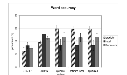
Figure 6: Word accuracy, Chasen and Juman vs. tango. The three rightmost groups show tango’s performance when parameters were tuned for different optimization criteria.

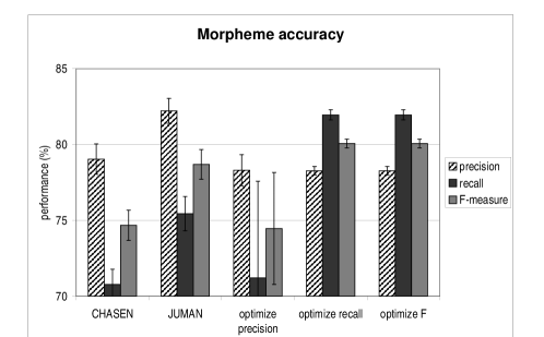
Figure 7: Morpheme accuracy, Chasen and Juman vs. tango.

Figure 6 shows word accuracy for Chasen, Juman, and our algorithm for parameter settings optimizing word precision, recall, and F-measure rates. As can be seen, in this case the choice of optimization criterion did not matter very much. tango achieves more than five percentage-points higher precision than Juman and Chasen. tango’s recall performance is also respectable in comparison to the morphological analyzers, falling (barely) between that of Juman and that of Chasen. Combined performance, as recorded by the F-measure, was about the same as Juman, and 4.22 percentage points higher than Chasen.

We also measured morpheme precision, recall, and F measure, all defined analogously to their word counterparts. Figure 7 shows the results. Unlike in the word accuracy case, the choice of training criterion clearly affected performance.

We see that tango’s morpheme precision was slightly lower than that of Chasen, and noticeably worse than for Juman. However, when we optimize for precision, the results for all three metrics are on average quite close to Chasen’s. tango’s recall results are substantially higher than for the morphological analyzers when recall was its optimization criterion. In terms of combined performance, tuning our algorithm for the F-measure achieves higher F-measure performance than Juman and Chasen, with the performance gain due to enhanced recall.

Thus, overall, we see that our method yields results rivalling those of morphological analyzers.

5.1.2 Compatible brackets results

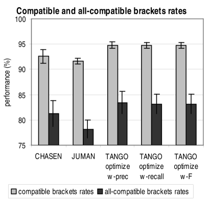
Figure 8: Compatible and all-compatible brackets rates, word-accuracy training.

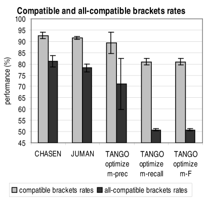
Figure 9: Compatible and all-compatible brackets rates, morpheme-accuracy training.

Figure 8 depicts the compatible brackets and all-compatible brackets rates for Chasen, Juman, and tango, using the three word accuracy metrics as training criteria for our method. tango  does better on the compatible brackets rate and the all-compatible brackets rates than the morphological analyzers do, regardless of training optimization function used.

The results degrade if morpheme accuracies are used as training criteria, as shown in Figure 9. Analysis of the results shows that most of the errors come from morpheme-dividing brackets: the parameters optimizing morpheme recall and F-measure are $N=\mbox{$\{2\}$}$ and $t=.5$, which leads to a very profligate policy in assigning boundaries.

5.1.3 Discussion

Overall, we see that our algorithm performs very well with respect to the morphological analyzers when word accuracies are used for training. At the morpheme level, the relative results for our algorithm in comparison to Chasen and Juman are mixed; recall and F are generally higher, but at the price of lower compatible brackets rates. The issue appears to be that single-character segments are common at the morpheme level because of affixes. The only way our algorithm can create such segments is by the threshold value, but too low a threshold causes precision to drop.

A manual (and quite tedious) analysis of the types of errors produced in the first test set reveals that the major errors our algorithm makes are mis-associating affixes (e.g., wrongly segmenting as ) and fusing single-character words to their neighbors (e.g. wrongly segmenting as ). Both of these are mistakes involving single characters, a problem just discussed. Another common error was the incorrect concatenation of family and given names, but this does not seem to be a particularly harmful error. On the other hand, the morphological analyzers made many errors in segmenting proper nouns, which are objects of prime importance in information extraction and related tasks, whereas our algorithm made far fewer of these mistakes.

In general, we conclude that tango produces high-quality word-level segmentations rivaling and sometimes outperforming morphological analyzers, and can yield morpheme accuracy results comparable to Chasen, although the bracket-metrics quality of the resultant morpheme-level segmentations is not as good. The algorithm does not fall prey to some of the problems in handling proper nouns that lexico-syntactic approaches suffer. Developing methods for improved handling of single-character morphemes would enhance the method, and is a direction for future work.

5.2 Comparison against sst

We further evaluated our algorithm by comparing it against another mostly-unsupervised algorithm: that of Sun, Shen, and Tsou [Sun, Shen, and Tsou,1998] (henceforth sst), which, to our knowledge, is the segmentation technique most similar to the one we have proposed. Our goal in these experiments was to investigate the null hypothesis that any reasonable $n$-gram-based method could yield results comparable to Chasen and Juman.

sst also performs segmentation without using a grammar, lexicon, or large amounts of annotated training data; instead, like tango, it relies on statistics garnered from an unsegmented corpus. Although Sun et al. implemented their method on Chinese (which also lacks space delimiters) instead of Japanese, they designed sst to be able to account for “two common construction types in Chinese word formation: ‘2 characters + 1 character’ and ‘1 character + 2 characters” (pg. 1269). As pointed out in Section 4.2.1 above, Japanese kanji compound words often have a similar structure [Takeda and Fujisaki,1987]; hence, we can apply sst to kanji as well, after appropriate parameter training.

5.2.1 The sst Algorithm

Like our algorithm, sst seeks to determine whether a given location constitutes a word boundary by looking for evidence of cohesion (or lack thereof) between the characters bordering the location. Recall the situation described by Figure 2: we have the character sequence “A B C D W X Y Z”, and must decide whether the location between D and W should be a boundary. The evidence sst uses comes from two sources. The first is the (pointwise or Fano) mutual information between D and W: $mi({\rm D},{\rm W})=\log(p({\rm D},{\rm W})/(p({\rm D})p({\rm W})))\,.$ The other statistic is the difference in t-score [Church and Hanks,1990] for the two trigrams CDW and DWX straddling the proposed boundary:

$$dts({\rm D},{\rm W})=\frac{p({\rm W}|{\rm D})-P({\rm D}|{\rm C})}{\sqrt{{\rm var}(p({\rm W}|{\rm D}))+{\rm var}(p({\rm D}|{\rm C}))}}-\frac{p({\rm X}|{\rm W})-P({\rm W}|{\rm D})}{\sqrt{{\rm var}(p({\rm X}|{\rm W}))+{\rm var}(p({\rm W}|{\rm D}))}}$$

Note that both the mutual information and the difference in t-score can be computed from character bigram statistics alone, as gathered from an unsegmented corpus.

Segmentation decisions are made based on a threshold $\theta$ on the mutual information, and on thresholds for the first and secondary local maxima and minima of the difference in t-score. There are six such free extremum parameters. In addition, we treated $\theta$ as another free parameter in our re-implementation; Sun et al. simply set it to the same value (namely, 2.5) that Sproat and Shih [Sproat and Shih,1990]) used. These seven parameters together yield a rather large parameter search space. For our implementation of the parameter training phase (Sun et al.’s paper does not give details), we set each of the six extremum thresholds to all the values in the set $\{0,50,100,150,200\}$ and the mutual information threshold to all values in the set $\{0,1.25,2.5,3.75,5\}$. Ties in training set performance — which were plentiful in our experiments — were broken by choosing smaller parameter values. We used the same count tables (i.e. with singleton $n$-grams deleted and unseen $n$-grams given a count of one) as for tango.

While local extrema and thresholds also play a important role in our method, we note that sst is considerably more complex than the algorithm we have proposed. Also observe that it makes use of conditional probabilities, whereas we simply compare frequencies.

5.2.2 sst Results

Figures 10 and 11 show the word and morpheme accuracy results. Clearly, sst does not perform as well as Juman at either level of segmentation granularity. Since the accuracy results are so much lower than the other algorithms, we do not apply the brackets metrics, for the reasons discussed above.

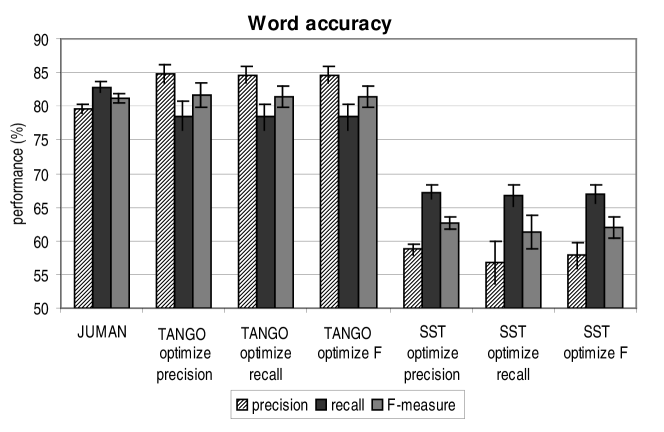
Figure 10: Word accuracy, Juman vs. tango vs. sst.

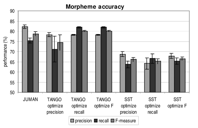
Figure 11: Morpheme accuracy, Juman vs. tango vs. sst.

It is clear that our algorithm outperforms sst, even though sst uses much more sophisticated statistics. Note that we incorporate $n$-grams of different orders, whereas sst essentially relies only on character bigrams, so at least some of the gain may be due to our using more sources of information from the unsegmented training corpus. We do not regard this as an unfair advantage because incorporating higher-order $n$-grams is easy to do for our method, and adds no conceptual overhead, whereas extending the mutual information to trigrams and larger $n$-grams can be a complex procedure [Magerman and Marcus,1990].

Stepping back, though, we note that our goal is not to emphasize the comparison with the particular algorithm sst, especially since it was developed for Chinese rather than Japanese. Rather, what we conclude from these experiments is that it is not necessarily easy for weakly-supervised statistical algorithms to do as well as morphological analyzers, even if they are given large amounts of unsegmented data as input and even if they employ well-known statistical functions. This finding further validates the tango algorithm.

5.3 Further Explorations

Given tango’s good performance in comparison to Chasen and Juman, we examined the role of the amount of parameter-training data tango is given as input, and investigated the contributions of the algorithm’s two parameters.

5.3.1 Minimal human effort is needed.

In contrast to our mostly-unsupervised method, morphological analyzers need a lexicon and grammar rules built using human expertise. The workload in creating dictionaries on the order of hundreds of thousands of words (the size of Chasen’s and Juman’s default lexicons) is clearly much larger than annotating the small parameter-training sets for our algorithm. tango also obviates the need to segment a large amount of parameter-training data because our algorithm draws almost all its information from an unsegmented corpus. Indeed, the only human effort involved in our algorithm is pre-segmenting the five 50-sequence parameter training sets, which took only 42 minutes. In contrast, previously proposed supervised approaches to Japanese segmentation have used annotated training sets ranging from 1000-5000 sentences [Kashioka et al.,1998] to 190,000 sentences [Nagata,1996a].

tango (50) tango (5) Juman (5) tango (5) tango (5) vs. vs. vs. vs. vs. Juman (50) Juman (5) Juman (50) tango (50) Juman (50) precision +5.27 +6.18 -1.04 -0.13 +5.14 recall -4.39 -3.73 -0.63 +0.03 -4.36 F-measure +0.26 +1.14 -0.84 +0.04 +0.30

Figure 12: Average relative word accuracy as a function of training set size. “5” and “50” denote training set size before discarding overlaps with the test sets.

To test how much annotated training data is actually necessary, we experimented with using miniscule parameter-training sets: five sets of only five strings each (from which any sequences repeated in the test data were discarded). It took only 4 minutes to perform the hand segmentation in this case.

Figure 12 shows the results. For instance, we see that training tango on five training sequences yielded 6.18 percentage points higher precision than using Juman with the same five training sequences; thus, our algorithm is making very efficient use of even very small training sets. The third data column proves that the information we provide Juman from the annotated training data does help, in that using smaller training sets results in lower performance. According to the fourth data column, performance doesn’t change very much if our algorithm gets only five training sequences instead of 50. Interestingly, the last column shows that if our algorithm has access to only five annotated sequences when Juman has access to ten times as many, we still achieve better precision and comparable F-measure.

5.3.2 Both the local maximum and threshold conditions contribute.

Recall that in our algorithm, a location $k$ is deemed a word boundary if the evidence $v_{N}(k)$ is either (1) a local maximum or (2) at least as big as the threshold $t$. It is natural to ask whether we really need two conditions, or whether just one would suffice. For instance, while $t$ is necessary for producing single-character segments, perhaps it also causes many recall errors, so that performance is actually better when the threshold criterion is ignored.

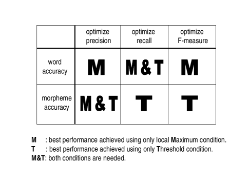
Figure 13: Entries indicate whether best performance is achieved using the local maximum condition (M), the threshold condition (T), or both.

We therefore studied whether optimal performance could be achieved using only one of the conditions. Figure 13 shows that in fact both contribute to producing good segmentations. Indeed, in some cases, both are needed to achieve the best performance; also, each condition when used in isolation yields suboptimal performance with respect to some performance metrics.

6 Related Work

6.1 Japanese Segmentation

Many previously proposed segmentation methods for Japanese text make use of either a pre-existing lexicon [Yamron et al.,1993, Matsumoto and Nagao,1994, Takeuchi and Matsumoto,1995, Nagata,1997, Fuchi and Takagi,1998] or a substantial amount of pre-segmented training data [Nagata,1994, Papageorgiou,1994, Nagata,1996a, Kashioka et al.,1998, Mori and Nagao,1998, Ogawa and Matsuda,1999]. Other approaches bootstrap from an initial segmentation provided by a baseline algorithm such as Juman [Matsukawa, Miller, and Weischedel,1993, Yamamoto,1996].

Unsupervised, non-lexicon-based methods for Japanese segmentation do exist, but often have limited applicability when it comes to kanji. Both Tomokiyo and Ries [Tomokiyo and Ries,1997] and Teller and Batchelder[Teller and Batchelder,1994] explicitly avoid working with kanji characters. Takeda and Fujisaki [Takeda and Fujisaki,1987] propose the short unit model, a type of Hidden Markov Model with linguistically-determined topology, for segmenting certain types of kanji compound words; in our five test datasets, we found that 13.56% of the kanji sequences contain words that the short unit model cannot handle.

Ito and Kohda’s [Ito and Kohda,1995] completely unsupervised statistical algorithm extracts high-frequency character $n$-grams as pseudo-lexicon entries; a standard segmentation algorithm is then used on the basis of the induced lexicon. But the segments so derived are only evaluated in terms of perplexity and intentionally need not be linguistically valid, since Ito and Kohda’s interest is not in word segmentation but in language modeling for speech.

6.2 Chinese Segmentation

There are several varieties of statistical Chinese segmentation algorithms that do not rely on syntactic information or a lexicon, and hence could potentially be applied to Japanese. One vein of work relies on the mutual information [Sproat and Shih,1990, Lua and Gan,1994]; sst can be considered a more sophisticated variant of these since it also incorporates t-scores. There are also algorithms that leverage pre-segmented training data [Palmer,1997, Dai, Loh, and Khoo,1999, Teahan et al.,2000, 1]. Finally, the unsupervised, knowledge-free algorithms of Ge, Pratt, and Smyth [Ge, Pratt, and Smyth,1999] and Peng and Schuurmans [Peng and Schuurmans,2001] both require use of the EM algorithm to derive the most likely segmentation; in contrast, our algorithm is both simple and fast.

7 Conclusion

In this paper, we have presented tango, a simple, mostly-unsupervised algorithm that segments Japanese sequences into words based on statistics drawn from a large unsegmented corpus. We evaluated performance on kanji with respect to several metrics, including the novel compatible brackets and all-compatible brackets rates, and found that our algorithm could yield performances rivaling that of lexicon-based morphological analyzers. Our experiments also showed that a similar previously-proposed mostly-unsupervised algorithm could not yield comparable results.

Since tango learns effectively from unannotated data, it represents a robust algorithm that is easily ported to other domains and applications. We view this research as a successful application of the (mostly) unsupervised learning paradigm: high-quality information can be extracted from large amounts of raw data, sometimes by relatively simple means.

On the other hand, we are by no means advocating a purely statistical approach to the Japanese segmentation problem. We have explicitly focused on long sequences of kanji as being particularly problematic for morphological analyzers such as Juman and Chasen, but these analyzers are well-suited for other types of sequences. We thus view our method, and mostly-unsupervised algorithms in general, as complementing knowledge-based techniques, and conjecture that hybrid systems that rely on the strengths of both kinds of methods will prove to be the most effective in the future.

References

- [1] Brent, Michael R. and Xiaopeng Tao. 2001. Chinese text segmentation with MBDP-1: Making the most of training corpora. In Proceedings of the ACL.
- [Church and Hanks,1990] Church, Kenneth Ward and Patrick Hanks. 1990. Word association norms, mutual information, and lexicography. Computational Linguistics, 16(1):22–29, March.
- [Cover and Thomas,1991] Cover, Thomas M. and Joy A. Thomas. 1991. Elements of Information Theory. Wiley series in telecommunications. Wiley-Interscience, New York.
- [Dai, Loh, and Khoo,1999] Dai, Yubin, Teck Ee Loh, and Christopher S. G. Khoo. 1999. A new statistical formula for Chinese text segmentation incorporating contextual information. In Proceedings of the 22nd SIGIR, pages 82–89.
- [Fuchi and Takagi,1998] Fuchi, Takeshi and Shinichiro Takagi. 1998. Japanese morphological analyzer using word co-occurrence - JTAG. In Proceedings of COLING-ACL ’98, pages 409–413.
- [Fung,1998] Fung, Pascale. 1998. Extracting key terms from Chinese and Japanese texts. Computer Processing of Oriental Languages, 12(1).
- [Ge, Pratt, and Smyth,1999] Ge, Xianping, Wanda Pratt, and Padhraic Smyth. 1999. Discovering Chinese words from unsegmented text. In Proceedings of the 22nd SIGIR, pages 271 – 272. Poster abstract.
- [Goldsmith,2001] Goldsmith, John. 2001. Unsupervised learning of the morphology of a natural language. Computational Linguistics, 27(2):153–198.
- [Grishman, Macleod, and Sterling,1992] Grishman, Ralph, Catherine Macleod, and John Sterling. 1992. Evaluating parsing strategies using standardized parse files. In Proceedings of the 3rd ANLP, pages 156–161.
- [Ito and Kohda,1995] Ito, Akinori and Kasaki Kohda. 1995. Language modeling by string pattern N-gram for Japanese speech recognition. In Proceedings of ICASSP.
- [Kashioka et al.,1998] Kashioka, Hideki, Yasuhiro Kawata, Yumiko Kinjo, Andrew Finch, and Ezra W. Black. 1998. Use of mutual information based character clusters in dictionary-less morphological analysis of Japanese. In Proceedings of COLING-ACL ’98, pages 658–662.
- [Kurohashi and Nagao,1999] Kurohashi, Sadao and Makoto Nagao. 1999. Japanese morphological analysis system JUMAN version 3.61 manual. In Japanese.
- [Lua,1995] Lua, Kim-Teng. 1995. Experiments on the use of bigram mutual information for Chinese natural language processing. In International Conference on Computer Processing of Oriental Languages(ICCPOL), pages 23–25.
- [Lua and Gan,1994] Lua, Kim-Teng and Kok-Wee Gan. 1994. An application of information theory in Chinese word segmentation. Computer Processing of Chinese and Oriental Languages, 8(1):115–123.
- [Magerman and Marcus,1990] Magerman, David M. and Mitchell P. Marcus. 1990. Parsing a natural language using information statistics. In Proceedings of AAAI, pages 984–989.
- [Manber and Myers,1993] Manber, Udi and Gene Myers. 1993. Suffix arrays: A new method for on-line string searches. SIAM Journal on Computing, 22(5):935–948.
- [Matsukawa, Miller, and Weischedel,1993] Matsukawa, T., Scott Miller, and Ralph Weischedel. 1993. Example-based correction of word segmentation and part of speech labelling. In Proceedings of the Human Language Technologies Workshop (HLT), pages 227–32.
- [Matsumoto et al.,1997] Matsumoto, Yuji, Akira Kitauchi, Tatsuo Yamashita, Yoshitaka Hirano, Osamu Imaichi, and Tomoaki Imamura. 1997. Japanese morphological analysis system ChaSen manual. Technical Report NAIST-IS-TR97007, Nara Institute of Science and Technology. In Japanese.
- [Matsumoto and Nagao,1994] Matsumoto, Yuji and Makoto Nagao. 1994. Improvements of Japanese morphological analyzer JUMAN. In Proceedings of the International Workshop on Sharable Natural Language Resources, pages 22–28.
- [Mori and Nagao,1998] Mori, Shinsuke and Makoto Nagao. 1998. Unknown word extraction from corpora using -gram statistics. Journal of the Information Processing Society of Japan, 39(7):2093–2100. In Japanese.
- [Nagao and Mori,1994] Nagao, Makoto and Shinsuke Mori. 1994. A new method of N-gram statistics for large number of n and automatic extraction of words and phrases from large text data of Japanese. In Proceedings of the 15th COLING, pages 611–615.
- [Nagata,1994] Nagata, Masaaki. 1994. A stochastic Japanese morphological analyzer using a forward-DP backward- n-best search algorithm. In Proceedings of the 15th COLING, pages 201–207.
- [Nagata,1996a] Nagata, Masaaki. 1996a. Automatic extraction of new words from Japanese texts using generalized forward-backward search. In Proceedings of the Conference on Empirical Methods in Natural Language Processing, pages 48–59.
- [Nagata,1996b] Nagata, Masaaki. 1996b. Context-based spelling correction for Japanese OCR. In Proceedings of the 16th COLING, pages 806–811.
- [Nagata,1997] Nagata, Masaaki. 1997. A self-organizing Japanese word segmenter using heuristic word identification and re-estimation. In Proceedings of the 5th Workshop on Very Large Corpora, pages 203–215.
- [Ogawa and Matsuda,1999] Ogawa, Yasushi and Toru Matsuda. 1999. Overlapping statistical segmentation for effective indexing of Japanese text. Information Processing and Management, 35:463–480.
- [Palmer,1997] Palmer, David. 1997. A trainable rule-based algorithm for word segmentation. In Proceedings of the 35th ACL/8th EACL, pages 321–328.
- [Papageorgiou,1994] Papageorgiou, Constantine P. 1994. Japanese word segmentation by hidden Markov model. In Proceedings of the Human Language Technologies Workshop (HLT), pages 283–288.
- [Peng and Schuurmans,2001] Peng, Fuchun and Dale Schuurmans. 2001. Self-supervised chinese word segmentation. In Advances in Intelligent Data Analysis (Proceedings of IDA-01), pages 238–247.
- [Saffran,2001] Saffran, Jenny R. 2001. The use of predictive dependencies in language learning. Journal of Memory and Language, 44:493–515.
- [Saffran, Aslin, and Newport,1996] Saffran, Jenny R., Richard N. Aslin, and Elissa L. Newport. 1996. Statistical learning by 8-month-old infants. Science, 274(5294):1926–1928, December.
- [Sproat and Shih,1990] Sproat, Richard and Chilin Shih. 1990. A statistical method for finding word boundaries in Chinese text. Computer Processing of Chinese and Oriental Languages, 4:336–351.
- [Sproat et al.,1996] Sproat, Richard, Chilin Shih, William Gale, and Nancy Chang. 1996. A stochastic finite-sate word-segmentation algorithm for Chinese. Computational Linguistics, 22(3):377–404.
- [Sun, Shen, and Tsou,1998] Sun, Maosong, Dayang Shen, and Benjamin K. Tsou. 1998. Chinese word segmentation without using lexicon and hand-crafted training data. In Proceedings of COLING-ACL, pages 1265–1271.
- [Takeda and Fujisaki,1987] Takeda, Koichi and Tetsunosuke Fujisaki. 1987. Automatic decomposition of kanji compound words using stochastic estimation. Journal of the Information Processing Society of Japan, 28(9):952–961. In Japanese.
- [Takeuchi and Matsumoto,1995] Takeuchi, Kouichi and Yuji Matsumoto. 1995. HMM parameter learning for Japanese morphological analyzer. In Proceedings of the 10th Pacific Asia Conference on Language, Information and Computation (PACLING), pages 163–172.
- [Teahan et al.,2000] Teahan, William J., Yingying Wen, Rodger McNab, and Ian H. Witten. 2000. A compression-based algorithm for Chinese word segmentation. Computational Linguistics, 26(3):275–393.
- [Teller and Batchelder,1994] Teller, Virginia and Eleanor Olds Batchelder. 1994. A probabilistic algorithm for segmenting non-kanji Japanese strings. In Proceedings of the 12th AAAI, pages 742–747.
- [Tomokiyo and Ries,1997] Tomokiyo, Laura Mayfield and Klaus Ries. 1997. What makes a word: learning base units in Japanese for speech recognition. In Proceedings of the ACL Special Interest Group in Natural Language Learning (CoNLL), pages 60–69.
- [Wu,1998] Wu, Dekai. 1998. A position statement on Chinese segmentation. http://www.cs.ust.hk/dekai/papers/segmentation.html. Presented at the Chinese Language Processing Workshop, University of Pennsylvania.
- [Wu and Su,1993] Wu, Ming-Wen and Keh-Yih Su. 1993. Corpus-based automatic compound extraction with mutual information and relative frequency count. In Proceedings of the R.O.C. Computational Linguistics Conference VI, pages 207–216.
- [Wu and Tseng,1993] Wu, Zimin and Gwyneth Tseng. 1993. Chinese text segmentation for text retrieval: Achievements and problems. Journal of the American Society for Information Science, 44(9):532–542.
- [Yamamoto,1996] Yamamoto, Mikio. 1996. A re-estimation method for stochastic language modeling from ambiguous observations. In Proceedings of the 4th Workshop on Very Large Corpora, pages 155–167.
- [Yamamoto and Church,2001] Yamamoto, Mikio and Kenneth W. Church. 2001. Using suffix arrays to compute term frequency and document frequency for all substrings in a corpus. Computational Linguistics, 27(1):1–30.
- [Yamron et al.,1993] Yamron, J., J. Baker, P. Bamberg, H. Chevalier, T. Dietzel, J. Elder, F. Kampmann, M. Mandel, L. Manganaro, T. Margolis, and E. Steele. 1993. LINGSTAT: An interactive, machine-aided translation system. In Proceedings of the Human Language Technologies Workshop (HLT), pages 191–195.