Computing Homotopic Shortest Paths Efficiently

Abstract

This paper addresses the problem of finding shortest paths homotopic to a given disjoint set of paths that wind amongst point obstacles in the plane. We present a faster algorithm than previously known.

0 Introduction

Finding Euclidean shortest paths in simple polygons is a well-studied problem. The funnel algorithm of Chazelle [3] and Lee and Preparata [10] finds the shortest path between two points in a simple polygon. Hershberger and Snoeyink [9] unify earlier results for computing shortest paths in polygons. They optimize a given path among obstacles in the plane under the Euclidean and link metrics and under polygonal convex distance functions. Related work has been done in addressing a classic VLSI problem, the continuous homotopic routing problem [4, 11]. For this problem it is required to route wires with fixed terminals among fixed obstacles when a sketch of the wires is given, i.e., each wire is given a specified homotopy class. If the wiring sketch is not given or the terminals are not fixed, the problem is NP-hard [12, 15, 16].

Some of the early work on continuous homotopic routing was done by Cole and Siegel [4] and Leiserson and Maley [11]. They show that in the $L_{\infty}$ norm a solution can be found in $O(k^{3}\log n)$ time and $O(k^{3})$ space, where $n$ is the number of wires and $k$ is the maximum of the input and output complexities of the wiring. Maley [13] shows how to extend the distance metric to arbitrary polygonal distance functions (including Euclidean distance) and presents a $O(k^{4}\log n)$ time and $O(k^{4})$ space algorithm. The best result so far is due to Gao et al. [8] who present a $O(kn^{2}\log(kn))$ time and $O(kn^{2})$ space algorithm. Duncan et al. [6] and Efrat et al. [7] present an $O(kn+n^{3})$ algorithm for the related fat edge drawing problem: given a planar weighted graph $G$ with maximum degree 1 and an embedding for $G$, find a planar drawing such that all the edges are drawn as thick as possible and proportional to the corresponding edge weights.

The topological notion of homotopy formally captures the notion of deforming paths. Let $\alpha,\beta:[0,1]\longrightarrow{{{R}}}^{2}$ be two continuous curves parameterized by arc-length. Then $\alpha$ and $\beta$ are homotopic with respect to a set of obstacles $V\subseteq{{R}}^{2}$ if $\alpha$ can be continuously deformed into $\beta$ while avoiding the obstacles; more formally, if there exists a continuous function $h:[0,1]\times[0,1]\rightarrow{{{R}}}^{2}$ with the following three properties:

1. $h(0,t)=\alpha(t)$ and $h(1,t)=\beta(t)$, for $0\leq t\leq 1$

2. $h(\lambda,0)=\alpha(0)=\beta(0)$ and $h(\lambda,1)=\alpha(1)=\beta(1)$ for $0\leq\lambda\leq 1$

3. $h(\lambda,t)\notin V$ for $0\leq\lambda\leq 1,0<t<1$

Let $\Pi=\{\pi_{1},\pi_{2},\dots,\pi_{n}\}$ be a set of disjoint, simple polygonal paths and let the endpoints of the paths in $\Pi$ define the set $T$ of at most $2n$ fixed points in the plane. Note that we allow a path to degenerate to a single point. We call the fixed points of $T$ “terminals,” and call the interior vertices of the paths “bends,” and use “points” in a more generic sense, e.g. “a point in the plane,” or “a point on a path.” We assume that no two terminals/bends lie on the same vertical line.

Our goal is to replace each path $\pi_{i}\in\Pi$ by a shortest path $\sigma_{i}$ that is homotopic to $\pi_{i}$ with respect to the set of obstacles $T$, see Fig. 1 and Fig. 3. Note that $\sigma_{i}$ is unique. Let $\Sigma=\{\sigma_{1},\ldots\sigma_{n}\}$ be the set of resulting paths. Observe that these output paths may [self] intersect by way of segments lying on top of each other, but will be non-crossing in the sense that a slight perturbation of the bends makes the paths simple and disjoint.

Let $k_{\it in}$ be the number of edges in all the paths of $\Pi$. Let $k_{\it out}$ be the number of edges in all the paths of $\Sigma$. We will measure the complexity of our algorithms in terms of $n$ and $k=\max\{k_{\it in},k_{\it out}\}$. In fact, the only relationship guaranteed among the parameters $n,k_{\it in},k_{\it out}$ is $k_{\it out}\leq nk_{\it in}$. Note that $k$ may be arbitrarily large compared to $n$. Clearly this is the case since, for example, a path can wind around a set of terminals arbitrarily many times. However, there exist non-trivial cases in which $k$ can be much larger than $n$. Even after shortest paths have been computed for each wire, $k$ can be as large as $k=\Omega(2^{n})$, see Fig. 1. The algorithm of Hershberger and Snoeyink [9] runs in time $O(nk)$. The algorithm presented in this paper runs in time $O(n^{2+\varepsilon}+k\log^{2}n)$, which is an improvement for $n<k$.

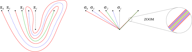
Figure 1: An example with exponential complexity: $k=\Omega(2^{n})$: On the left is the initial wiring sketch, and on the right is the wiring after the shortest paths have been computed. The number of edge segments in the shortest paths $\sigma_{1},\sigma_{2},\sigma_{3},\sigma_{4}$ is $1,2,4,8$, respectively. In general, wire $\sigma_{i}$ has $2^{i-1}$ edge segments. Note that on the right many edge segments are parallel.

Although $k$ can be arbitrarily large compared to $n$, one easily forms the intuition that, because the paths are simple and disjoint, $k$ can be large in a non-trivial way only because path sections are repeated over and over. For example, a path may spiral arbitrarily many times around a set of points, but each wrap around the set is the same.

Our method makes essential use of this observation. We do not begin by explicitly searching for repeated path sections—this seems difficult modulo homotopic equivalence. Instead we begin in section 2 by applying vertical shortcuts to the paths (homotopically) so that each left and each right local extreme point occurs at a terminal. These terminals must then be part of the final shortest paths, and we have decomposed the paths into $x$-monotone pieces with endpoints at terminals. In section 3 we argue that the number of homotopically distinct $x$-monotone pieces is at most $O(n)$. We will bundle together all the homotopically equivalent pieces. Routing one representative from each such bundle using the straightforward “funnel” technique takes $O(k+n^{2})$ time total. In section 3 we reduce this using a “shielding technique” where we again exploit the fact that the paths are disjoint and use the knowledge gained in routing one shortest path to avoid repeating work when we route subsequent paths. The final step of the algorithm is to unbundle, and recover the final paths by putting together the appropriate pieces. We summarize the main steps of the algorithm in Fig. 2.

Main Algorithm 1. shortcut paths to divide into monotone pieces 2. bundle homotopically equivalent pieces 3. find the shortest path for each bundle 4. unbundle to recover final paths

Figure 2: Summary of the algorithm.

Before we turn to the remainder of the paper, which consists of one section for each of steps 1, 2, and 3, it is worth noting that we rely on some powerful techniques. In step 1, we use simplex range search queries to perform homotopic simplifications on the paths. To do this, we use Chazelle’s cutting trees data structure [2]. In step 2 we need to identify homotopically equivalent monotone path pieces. We use the efficient trapezoidization algorithm of Bar-Yehuda and Chazelle [1] to perform this step. Step 3 uses ideas from “funnel” algorithms for shortest paths [10]. Step 4 is straight-forward.

We will find it convenient to regard each terminal as a small diamond. Otherwise when a vertical shortcut goes through a terminal we will need to specify whether the path actually goes to the left or the right of the terminal, which is awkward to say and to draw.

1 Shortcutting to Divide Paths into Monotone Pieces

We begin by applying vertical shortcuts to reduce each path to a sequence of $x$-monotone path sections, see Fig. 3. A vertical shortcut is a vertical line segment $ab$ joining a point $a$ on some path $\pi$ with a point $b$ also on $\pi$, and with the property that the subpath of $\pi$ joining $a$ and $b$, $\pi_{ab}$, is homotopic to the line segment $ab$.

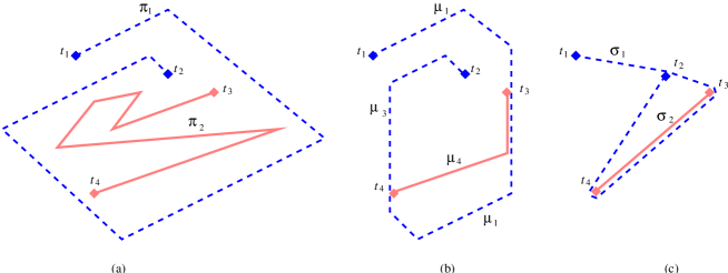
Figure 3: (a) Two paths $\pi_{1}$ and $pi_{2}$ joining terminals $t_{1}$ to $t_{2}$ and $t_{3}$ to $t_{4}$, respectively. (b) The two paths after performing vertical shortcuts. Note that path $\pi_{1}$ now consists of 3 monotone pieces: $\mu_{1}$ from $t_{1}$ to $t_{3}$, $\mu_{2}$ from $t_{3}$ to $t_{4}$, and $\mu_{3}$ from $t_{4}$ to $t_{2}$; path $\pi_{2}$ now consists of one $x$-monotone piece, $\mu_{4}$, homotopically equivalent to $\mu_{2}$; (c) The final homotopically equivalent shortest paths, $\sigma_{1}$ and $\sigma_{2}$.

We will only do elementary vertical shortcuts where the subpath $\pi_{ab}$ consists of [portions of] 2 line segments or 3 line segments with the middle one vertical, and the other two non-vertical. We distinguish left shortcuts which are elementary vertical shortcuts where $\pi_{ab}$ contains a point to the left of the line through $ab$; right shortcuts where $\pi_{ab}$ contains a point to the right of the line through $ab$; and collinear shortcuts where $\pi_{ab}$ lies in the line through $ab$, see Fig. 4 and Fig. 5. Collinear shortcuts are always applied after left/right shortcuts (and only then), and prevent consecutive vertical segments.

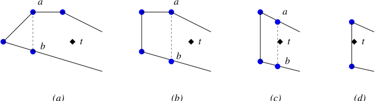
Figure 4: Maximal left shortcuts (bends are represented by circles and terminals by diamonds): (a) a 2 segment shortcut, maximal because $a$ is a bend; (b) a 3 segment shortcut, maximal for the same reason; (c) a 3 segment shortcut, maximal because $ab$ hits a terminal; (d) the result of the shortcut in (c).

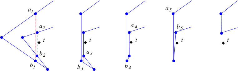
Figure 5: A sequence of maximal elementary vertical shortcuts (bends are represented by circles and terminals by diamonds). Shortcuts $a_{1}b_{1}$ and $a_{2}b_{2}$ are left shortcuts; $a_{3}b_{3}$ is a right shortcut; and $a_{4}b_{4}$ and $a_{5}b_{5}$ are collinear shortcuts.

We will in fact only apply maximal elementary vertical shortcuts, where the subpath $\pi_{ab}$ cannot be increased. In particular, this means that for left and right shortcuts, either $a$ or $b$ is a bend, or the line segment $ab$ hits a terminal.

A local left [right] extreme of a path is a point or, more generally, a vertical segment, where the $x$-coordinate of the path reaches a local min [max]. Observe that every left [right] shortcut “cuts off” a local left [right] extreme. Conversely, every left [right] local extreme provides a left [right] shortcut unless the local extreme is locked at a terminal, meaning that the left [right] extreme contains the left [right] point of the terminal’s diamond. Figure 4 shows 4 cases of left extremes; in (a–c) they provide left shortcuts, but in case (d) the left extreme is locked at a terminal.

We will use range searching to detect, for a local left extreme, $l$, the maximal left shortcut that can be performed there. In particular, given $l$, we first identify the maximal potential shortcut in the absence of terminals. To do this, take the segment preceding $l$ and the segment following $l$ along the path. Take their right endpoints, and let $t$ be the leftmost of these two points. Then $t$ determines the maximal potential shortcut that can be performed at $l$. This potential shortcut forms either a triangle (for example, triangle $abl$ in Figure 4(a)) or a trapezoid (for example, the trapezoid determined by $a$, $b$, and $l$, in Figure 4(b)). If a range query tells us that the triangle/trapezoid is free of terminals, then it forms the true maximal shortcut from $l$. Otherwise, the range query should tell us the leftmost terminal inside the triangle/trapezoid, and that determines the maximal left shortcut from $l$. Note that the ranges we need to query are triangles with one vertical side, and trapezoids with two vertical sides.

Our algorithm is to perform elementary vertical shortcuts until none remain, at which time all local left and right extremes are locked at terminals, so the path divides into monotone pieces. See Section 1.2 for justification. Doing elementary vertical shortcuts in an arbitrary order may result in crossing paths as shown in Fig. 7; to guarantee non-crossing paths we will do the elementary vertical shortcuts in alternating left and right phases, where a left [right] phase means we do left [right] shortcuts (and the consequent collinear shortcuts) until no more are possible. See Section 1.3 for justification. We summarize these steps in Fig. 6.

ShortCut traverse paths initializing $L$ $\leftarrow$ $\{$local left extremes not locked at terminals$\}$ $R$ $\leftarrow$ $\{$local right extremes not locked at terminals$\}$ Loop LeftPhase RightPhase Until $L$ and $R$ are empty LeftPhase While $L$ is non-empty $l\leftarrow$ remove an element of $L$ $\tau\leftarrow$ the triangle/trapezoid forming the maximal potential shortcut at $l$ RangeQuery($\tau$) If $\tau$ is empty of terminals $s\leftarrow$ right side of $\tau$ Else $s\leftarrow$ leftmost terminal inside $\tau$ do a left shortcut of $\tau$ to $s$ perform consequent collinear shortcuts If any right local extremes disappear, remove them from $R$ If the final vertical segment is a local left [right] extreme and not locked at a terminal add it to $L$ [$R$, resp.] RightPhase (defined analogous to LeftShortcut but with “left” and “right” exchanged)

Figure 6: Pseudo-code for the shortcutting phase of the algorithm.

Figure 7: Performing shortcuts in arbitrary order may result in crossings. (a) Two disjoint paths $w_{1}$ and $w_{2}$; (b) After a left shortcut in $w_{1}$ and a right shortcut in $w_{2}$ there is a crossing. Note that no further shortcuts are possible for either path, and hence the crossing cannot be removed; (c) If both shortcuts are right [left] there are no crossings.

The remainder of this section consists of four subsections: Subsection 1.1 justifies organizing the above algorithm around the sets of left and right extremes, rather than explicitly searching each time for a shortcut to perform. Subsection 1.2 establishes the fact that performing elementary vertical shortcuts enables us to divide the paths into $x$-monotone pieces with endpoints at terminals. Subsection 1.3 argues that doing elementary vertical shortcuts in left/right phases prevents crossings. Finally, Subsection 1.4 deals with implementation and run-time analysis.

1.1 Correctness

The point of this section is to show that the above algorithm correctly maintains the sets $L$ and $R$ of local left and right extremes not locked at terminals. Consider a left phase. The set $R$ is explicitly updated whenever it changes. For the correctness of $L$ we use:

Claim 1.1

Doing one left shortcut does not alter other local left extremes, nor the shortcuts that will be performed there.

Proof: A left shortcut only removes left portions of non-vertical segments.

 

We note that a similar claim fails for collinear shortcuts: doing one may prevent others.

1.2 Correctness of division into monotone pieces

Claim 1.2

At the end of a left [right] phase of shortcuts, each local left [right] extreme is locked at a terminal.

We note that more than one left and one right phase may be required, since the right phase may add new members to $L$, see Fig. 8.

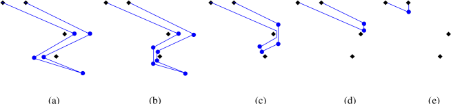
Figure 8: A path going through alternating left and right shortcutting phases: (a) the original path; (b) after a left phase; (c) after a right phase; (d) after a left phase; (e) after a right phase.

Claim 1.3

Let $\pi$ be a path, and let $\mu$ be a result of performing left and right phases of elementary vertical shortcuts on $\pi$ until no more are possible. Suppose that the local left and right extremes of $\mu$ are locked at the terminals $t_{i_{1}},\ldots,t_{i_{l}}$ in that order. Let $\sigma$ be a shortest path homotopic to $\pi$. Then the local left [right] extremes of $\sigma$ are locked at exactly the same ordered list of terminals, and furthermore, the portion of $\sigma$ between $t_{i_{j}}$ and $t_{i_{j+1}}$ is a shortest path homotopic to the portion of $\mu$ between those same terminals.

Proof Sketch: Because $\pi$ and $\mu$ are homotopic, $\sigma$ is the shortest path homotopic to $\mu$. We can thus go from $\mu$ to $\sigma$ using “rubber band” deformations that only shorten the path, and such deformations cannot loosen a left [right] extreme from the terminal it is locked at.

 

1.3 Non-crossing paths

The purpose of this section is to prove the following:

Lemma 1.4

Each left [right] phase of shortcuts preserves the property that paths are non-crossing.

By symmetry, we can concentrate on a left phase. Note that a left phase, as we have described it, is non-deterministic. At each stage we choose one member $l$ from the set $L$ of current local left extremes, and use it to perform a left shortcut. To prove the Lemma we will first show that for each left phase there is some sequence of choices that preserves the property that the paths are non-crossing. We will then argue that the end result of a phase does not depend on the choices made.

Claim 1.5

Suppose we have a set of non-crossing paths. Let $L$ be the current set of local left extremes not locked at terminals, and let $l\in L$ be a rightmost element of $L$. Performing the shortcut for $l$ (together with any consequent collinear shortcuts) leaves the paths non-crossing.

Observe that we can—at least in theory—complete a left phase of shortcuts using this “rightmost” order. In practice we choose not to do this simply because of the extra time required to maintain a heap.

Lemma 1.6

The end result of a left phase does not depend on the sequence of choices made during the phase.

Proof: We begin with the claim that the set $\cal L$ of all local left extremes that appear in $L$ over the course of the phase is independent of the choices made during the phase.

This implies that the set of left shortcuts performed during the course of the phase is also independent of the choices made during the phase. However, the set of collinear shortcuts is not independent. In particular, the order in which we perform left shortcuts affects the set of collinear shortcuts, see Fig. 9.

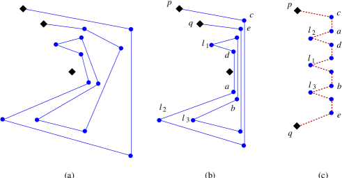
Figure 9: (a) A given path undergoes a right phase; (b) Handling local left extreme $l_{1}$ first yields the shortcut $ab$. Handling the local left extreme $l_{2}$ first yields shortcut $cd$. The final result of handling $l_{1}$, $l_{2}$ and $l_{3}$ in any order is shortcut $ce$; (c) An “unfolded” version of part (b).

Consider one left phase. Let $L_{0}$ be the initial set of local left extremes not locked at terminals. Let $\cal L$ be the union of $L$ over the course of the phase. Suppose two sequences of choices $C_{1}$ and $C_{2}$ during a left phase yield sets ${\cal L}_{1}$ and ${\cal L}_{2}$. We would like to show that ${\cal L}_{1}={\cal L}_{2}$. Consider $l\in{\cal L}_{1}$. We will prove $l\in{\cal L}_{2}$ by induction on the number of left shortcuts performed in the phase before $l$ enters ${\cal L}_{1}$. If this number is 0 then $l\in L_{0}$ and we are done. Otherwise, $l$ is added to $L$ as a result of some left shortcut and consequent collinear shortcuts. Any vertical segment used in the collinear shortcuts may, in its turn, have arisen as a result of some left shortcut and consequent collinear shortcuts. Tracing this process, we find that $l$ is formed from a set of left shortcuts linked by vertical segments, all in the same vertical line as $l$, see Fig. 9. All these left shortcuts arose from local left extremes that entered ${\cal L}_{1}$ before $l$ did, and thus, by induction, are in ${\cal L}_{2}$. By Claim 1.1 left shortcuts are performed at each of these during the choice sequence $C_{2}$—though possibly in a different order than in $C_{1}$. The consequent collinear shortcuts will merge all the verticals forming $l$, and cannot merge more than that because the segments attached before and after $l$ are not vertical ($l$ is a local left extreme). Thus $l$ is in ${\cal L}_{2}$.

This proves that the set of local left extremes, and thus the set of left shortcuts is independent of choices made during the phase. Any vertical segment that is in the final set of paths output by the phase arises through left shortcuts plus consequent collinear shortcuts. Since any set of choices leads to the same set of left shortcuts, though possibly in different order, the consequent collinear shortcuts will arrive at the same final vertical shortcuts—i.e. the same final paths.

 

1.4 Implementation and run-time analysis

In order to perform range queries we need the cutting trees data structure of Chazelle [2]. The cutting trees can be constructed in $O(n^{2+\varepsilon})$ time and space, where $\varepsilon$ is an arbitrarily small constant, and they support simplex range queries in time $O(\log n)$  [2]. (Note that a trapezoid is a union of two triangles.) In case a triangle that we query is not empty, we need to find the rightmost/leftmost terminal inside it. To do this, create a segment tree ${\cal T}$ on the $x$-projections of the terminals, and maintain a cutting tree on each node of ${\cal T}$. This enables us to find the rightmost/leftmost terminal inside a query triangle in time $O(\log^{2}n)$, without increasing the asymptotic space and preprocessing time. Details are standard and omitted from this abstract.

Claim 1.7

The number of elementary vertical shortcuts that can be applied to a set of paths with a total of $k$ segments is at most $2k$.

Proof: Assume that no two terminals and/or bends line up vertically. Consider the set of vertical lines through bends and through the left and right sides of each terminal’s diamond. An elementary shortcut operates between two of these vertical lines. If a left [right] shortcut has its leftmost [rightmost] vertical at a bend, then after the shortcut, this vertical disappears forever, see Fig. 5. There are thus at most $k$ such elementary shortcuts. Consider, on the other hand, a left shortcut that has its leftmost vertical at a terminal. This only occurs when two previous left shortcuts are stopped at the terminal, and then combined in a collinear shortcut. See the right hand pictures of Fig. 5. Thus an original edge of the path has disappeared. Note that elementary shortcuts never fragment an edge of the path into two edges, but only shorten it from one end or the other. Thus there are at most $k$ elementary shortcuts of this type. Altogether, we obtain a bound of $2k$ elementary shortcuts.

 

This implies the following simple corollary:

Corollary 1.8

The running time of the shortcutting phase, not counting the preprocessing to construct cutting trees, is $O(k\log^{2}n)$.

Including preprocessing, step 1 takes time $O(n^{2+\varepsilon}+k\log^{2}n)$.

2 Bundling Homotopically Identical Paths

Let $M=\{\mu_{1}\dots\mu_{m}\}$ be the set of $x$-monotone paths obtained from step 1 of our algorithm. In the second step of the algorithm we bundle homotopically equivalent paths in $M$. More precisely, we take one representative path for each equivalence class of homotopically equivalent paths in $M$. This is justified because the paths in each equivalence class have the same homotopic shortest path. Because the paths in $M$ are non-crossing and $x$-monotone, it is easier to detect homotopic equivalence: two paths are homotopically equivalent if they have the same endpoints, and, between these endpoints no terminal lies vertically above one path and vertically below the other.

In order to perform the bundling we use a trapezoidization of $M$, see Fig. 10. We apply the trapezoidization algorithm of Bar-Yehuda and Chazelle [1] to the paths obtained after the shortcuts of step 1, but before these paths are chopped into monotone pieces.

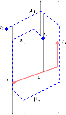
Figure 10: A trapezoidization enables us to identify that $\mu_{2}$ and $\mu_{4}$ are homotopically equivalent.

Claim 2.1

We can perturb the paths output from step 1 so that they become disjoint and the Bar-Yehuda and Chazelle algorithm can be applied.

The trapezoidization algorithm takes time $O(k+n(\log n)^{1+\varepsilon})$, which is bounded by the time taken by step 1. Once we have a trapezoidization of $M$, we bundle homotopically equivalent paths as follows. While scanning each $\mu\in M$, we check if it is homotopically equivalent to the path “below” it, by examining all the edges of the trapezoidization that are incident to $\mu$ from below. If all these trapezoidization edges reach the same path $\mu_{j}$ and none pass through a terminal on the way to $\mu_{j}$, and $\mu_{i}$ and $\mu_{j}$ have the same terminals as endpoints, then we mark $\mu_{i}$ as a duplicate. Let $R=\{\rho_{1}\dots\rho_{r}\}$ be the paths of $M$ that are not marked as duplicates.

Lemma 2.2

The number of paths in $R$ is bounded by $2n$.

Proof: Note that every terminal $t$ is either a right endpoint of paths in $R$ or a left endpoint of paths in $R$, but not both. This is because a terminal cannot have local left extremes and local right extremes locked at it without the paths crossing.

For each terminal $t\in T$, associate its bottommost incident path $\phi(t)$ (its “floor”), and the first path hit by a vertical ray going up from $t$, $\gamma(t)$ (its “roof”). We claim that every path in $R$ is $\phi(t)$ or $\gamma(t)$ for some $t\in T$. This proves that the number of paths in $R$ is at most $2n$.

Consider a path $\rho\in R$ with left and right terminals $s$ and $t$, respectively. Suppose that $\rho$ is not a roof. Then every vertical ray extending downward from a point of $\rho$ must hit the same path $\sigma$. (If two rays hit different paths, then in the middle some ray must hit a terminal.) Furthermore, since $\rho$ is not the bottommost path incident to $s$, $\sigma$ must hit $s$. Similarly $\sigma$ must hit $t$. But then $\sigma$ and $\rho$ are homotopically equivalent.

 

3 Shortest Paths

In this section we find shortest paths homotopic to the $O(n)$ monotone paths $R=\{\rho_{1},\ldots,\rho_{r}\}$ produced in the previous section. Let $\rho^{\prime}_{i}$ denote the shortest path homotopic to $\rho_{i}$. We route each path using a funnel technique. The funnel algorithm of [3] and [10] operates on a triangulation of the $n$ points (the terminals in our case), and follows the path through the triangulation maintaining a current “funnel” containing all possible shortest paths to this point. The algorithm takes time proportional to the number of edges in the path plus the number of intersections between the triangulation edges and the path.

Rather than a triangulation, we will use a trapezoidization formed by passing a vertical line through each of the $n$ terminals, see Fig. 11(a). Then, since each path $\rho_{i}$ is $x$-monotone, it has $O(n)$ intersections with trapezoid edges, and the funnel algorithm takes time $O(n+k_{i})$, where $k_{i}$ is the number of edges in $\rho_{i}$. This gives a total over all paths of $O(n^{2}+k)$. Recall that $k$ is $\max\{k_{\it in},k_{\it out}\}$, where $k_{\it in}$ is the number of edges in all the input paths, and $k_{\it out}$ is the number of edges in all the output paths. Note that the number of edges in $R$ is bounded by $k_{\it in\/}$.

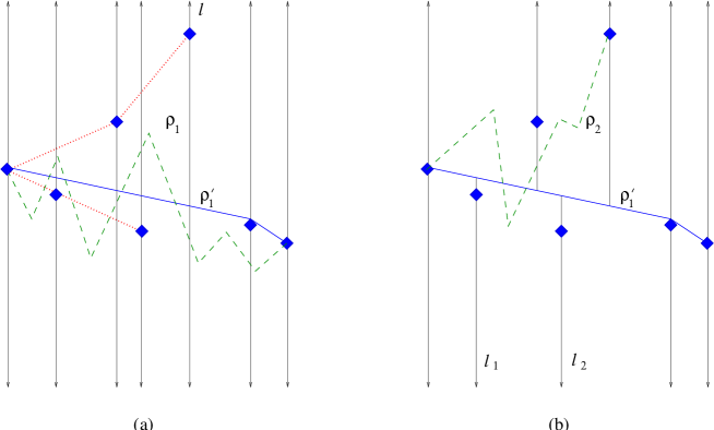
Figure 11: (a) A path $\rho_{1}$ (dashed), its funnel up to line $l$ (dotted) and the final homotopic shortest path $\rho^{\prime}_{1}$; (b) After the shortest path $\rho^{\prime}_{1}$ has been found, shielding allows us to route another path $\rho_{2}$ without examining vertical lines $l_{1}$ and $l_{2}$.

With respect to our whole algorithm, this time of $O(n^{2}+k)$ is dominated by the $O(n^{2+\varepsilon})$ time required to create the range query data structure in step 1. However, it is interesting to see how much improvement we can make in this step alone. In the remainder of this section we describe a randomized algorithm to route the $O(n)$ monotone paths of $R$ in time $O(n\log n+k)$, and finally mention a deterministic algorithm with $O(n\sqrt{n}+k)$ running time.

Both methods use a “shielding” technique. We begin by describing this idea intuitively. First note that the $\rho_{i}$’s can be routed independently, since none affects the others. The initial paths $\rho_{i}$ are non-crossing, and so are the final shortest paths, $\rho^{\prime}_{i}$. If $\rho_{j}$ is below $\rho_{i}$, and we have already computed $\rho^{\prime}_{j}$, then $\rho^{\prime}_{j}$ behaves as a barrier that “shields” $\rho_{i}$ from terminals that are vertically below $\rho^{\prime}_{j}$, see Fig. 11(b).

To utilize shielding we will modify the basic trapezoidization described above as we discover shortest paths $\rho^{\prime}_{i}$. In particular, the upward vertical ray through terminal $t$, $u(t)$, will be truncated at the lowest shortest path $\rho^{\prime}_{i}$ that is strictly above $t$ and does not bend at $t$. The downward vertical ray through terminal $t$, $d(t)$, will be truncated in an analogous way.

The shortest paths found so far, together with the truncated vertical rays $u(t)$ and $d(t)$ for each terminal $t$, partition the plane into trapezoids, each bounded from left and right by the vertical rays, and from above and below by shortest paths. To route a new path $\rho_{i}$ through this modified trapezoidization we use the following algorithm.

Routing $\rho_{i}$ with shielding

1. Identify the first trapezoid that $\rho^{\prime}_{i}$ will traverse. This can be done in $O(\log n)$ time because the shortest paths observe the same vertical ordering as the original $\rho_{j}$’s.

2. Traverse from left to right the sequence of trapezoids that $\rho^{\prime}_{i}$ will pass through. (Note that $\rho_{i}$ itself may pass through different trapezoids, see Fig. 11(b).) We construct the funnel for $\rho^{\prime}_{i}$ as we do this traversal. Suppose that our path enters trapezoid $\tau$. To leave $\tau$ on the right we have two cases. If the right side of $\tau$ is a point, then it is a terminal $t$, and we are locked between two paths that terminate or bend at $t$. Then the funnel collapses to this point, and we proceed to the next trapezoid if $\rho_{i}$ continues. Otherwise the right side of $\tau$ is a vertical through some terminal $t$, and (unless $\rho_{i}$ ends at $t$) we have a choice of two trapezoids to enter, the upper one with left side $u(t)$ or the lower one with left side $d(t)$. We follow path $\rho_{i}$ until it crosses the infinite vertical line through $t$. If it passes above $t$ then we enter the upper trapezoid, and otherwise we enter the lower trapezoid. We update the funnel to include $t$.

3. When we reach the right endpoint of $\rho_{i}$, the funnel gives us the shortest homotopic path $\rho^{\prime}_{i}$.

4. We update the trapezoidization as follows. For each vertical segment $u(t)$ or $d(t)$ that is intersected by $\rho^{\prime}_{i}$ we chop the segment at its intersection point with $\rho_{i}^{\prime}$, provided that the intersection point is not $t$ (i.e. that $\rho_{i}^{\prime}$ does not bend at or terminate at $t$).

Without yet discussing the order in which we route the paths, we can say a bit about the timing of this shielding method. As we traverse a path $\rho_{i}$ we spend time proportional to the size of $\rho_{i}$ plus the number of trapezoids traversed by $\rho^{\prime}_{i}$. When $\rho^{\prime}_{i}$ leaves a trapezoid, say at the line segment $u(t)$ above terminal $t$, it may happen that $\rho^{\prime}_{i}$ will bend at $t$ or terminate at $t$. In this case $t$ is part of the output path $\rho^{\prime}_{i}$, and we can charge the work for this trapezoid to the output size. If, on the other hand, $\rho^{\prime}_{i}$ does not bend or terminate at $t$, then it crosses $u(t)$ and we chop $u(t)$ there. In this case we charge the work for this trapezoid to the chop. Thus the total time spent by the algorithm is $O(k+C)$ where $C$ is the total number of chops performed at the $n$ verticals.

For shielding to be effective we need to route paths in an order that makes $C$ grow more slowly than $n^{2}$. We first analyze the randomized algorithm where we choose the next path to route at random with uniform probability from the remaining paths.

Claim 3.1

If paths are routed in random order then the expected number of times we chop a segment $u(t)$ or $d(t)$ is $O(\log r)$, and thus $C$ is $O(n\log n)$, and the routing takes time $O(k+n\log n)$.

Proof: This follows from a standard backward analysis. See for example [5] for other proofs along these lines. Let $l$ be a vertical line through a point $t$, and let $u$ denote a ray emerging vertically from $t$. Assume that $m$ paths intersecting $u$ have been inserted up to now, and we are about to insert a new one. Then $u$ will be chopped if and only if the new path creates an intersection point below all existing intersection points on $u$, but above $t$ itself. Since the order of the insertions is random, the probability of the new intersection point being below all other intersection points is $1/m$. Summing over all paths yields the claimed bound.

 

Finally, we mention that we can achieve a routing time of $O(k+n\sqrt{n})$ deterministically. Suppose that the paths $\{\rho_{1},\ldots,\rho_{r}\}$ are in order from top to bottom. (We get this for free from step 2 of our algorithm.) Partition the paths into blocks $B_{1},\ldots,B_{\sqrt{r}}$ each of size $\sqrt{r}$, and route them one block at a time from $B_{\sqrt{r}}$ to $B_{1}$. Within each block we process the paths in order. Since the largest increasing [decreasing] sequence with this ordering has size $\sqrt{r}$, therefore the number of chops at each vertical is $\sqrt{r}$. Thus $C$ is $O(n\sqrt{n})$, and this routing method takes time $O(k+n\sqrt{n})$.

4 Conclusion and Open Problems

For any set of $n$ disjoint paths joining pairs of terminals in the plane we can find shortest paths homotopic with respect to the set of terminals in time $O(n^{2+\varepsilon}+k\log^{2}n)$ where $k$ is the sum of input and output sizes of the paths. If $k$ is larger than $n$ this is better than the Hershberger-Snoeyink algorithm which runs in time $O(nk)$.

More generally, we can use any other range search method, and obtain a running time of $O(P+kQ+n(\log n)^{1+\varepsilon}+T)$ where $P$ is the preprocessing time for the range search data structure on $n$ points, $Q$ is the time for a simplex optimization query (find the minimum/maximum $x$-coordinate point in a triangle), and $T$ is the time for the shortest path method of step 3—$O(n\log n)$ randomized, or $O(n\sqrt{n})$ deterministic. Whether $k$ is large or small compared to $n$ determines which trade-off between $P$ and $Q$ is preferred. For example, the partition tree method of Matoušek [14] yields an emptiness query time of $O(\sqrt{n})$ with near-linear time preprocessing, and would be preferable for $k=O(n^{3/2})$. With any approach to range searching, it may be possible to improve the query time by taking into account the fact that one of the edges of each query triangle is vertical.

Another open problem is whether we can do without range queries, and somehow use a trapezoidization of the original paths, since this can be found so efficiently with the Bar-Yehuda and Chazelle algorithm.

References

- [1] R. Bar-Yehuda and B. Chazelle. Triangulating disjoint Jordan chains. International Journal of Computational Geometry & Applications, 4(4):475–481, 1994.
- [2] Chazelle. Cutting hyperplanes for divide-and-conquer. Discrete & Computational Geometry, 9:145–158, 1993.
- [3] B. Chazelle. A theorem on polygon cutting with applications. In 23th Annual Symposium on Foundations of Computer Science, pages 339–349, Los Alamitos, Ca., USA, Nov. 1982. IEEE Computer Society Press.
- [4] R. Cole and A. Siegel. River routing every which way, but loose. In 25th Annual Symposium on Foundations of Computer Science, pages 65–73, Los Angeles, Ca., USA, Oct. 1984. IEEE Computer Society Press.
- [5] M. de Berg, M. van Kreveld, M. H. Overmars, and O. Schwarzkopf. Computational Geometry: Algorithms and Applications. Springer-Verlag, 2nd edition, 2000.
- [6] C. A. Duncan, A. Efrat, S. G. Kobourov, and C. Wenk. Drawing with fat edges. In 9th Symposium on Graph Drawing (GD’01), pages 162–177, September 2001.
- [7] A. Efrat, S. G. Kobourov, M. Stepp, and C. Wenk. Growing fat graphs. In Proceedings of the 18th Annual Symposium on Computational Geometry, 2002. Video submission. To appear.
- [8] S. Gao, M. Jerrum, M. Kaufmann, K. Mehlhorn, W. Rülling, and C. Storb. On continuous homotopic one layer routing. In Proceedings of the 4th Annual Symposium on Computational Geometry, pages 392–402, New York, 1988. ACM Press.
- [9] Hershberger and Snoeyink. Computing minimum length paths of a given homotopy class. CGTA: Computational Geometry: Theory and Applications, 4:63–97, 1994.
- [10] D. T. Lee and F. P. Preparata. Euclidean shortest paths in the presence of rectilinear barriers. Networks, 14(3):393–410, 1984.
- [11] C. E. Leiserson and F. M. Maley. Algorithms for routing and testing routability of planar VLSI layouts. In Proceedings of the 17th Annual ACM Symposium on Theory of Computing, pages 69–78, 1985.
- [12] C. E. Leiserson and R. Y. Pinter. Optimal placement for river routing. SIAM Journal on Computing, 12(3):447–462, Aug. 1983.
- [13] F. M. Maley. Single-Layer Wire Routing. PhD thesis, Massachusetts Institute of Technology, 1987.
- [14] J. Matošek. Range searching with efficient hierarchical cuttings. Discrete & Computational Geometry, 10:157–182, 1993.
- [15] R. Pinter. River-routing: Methodology and analysis. In R. Bryant, editor, Third Caltech Conference on VLSI. Computer Science Press, 1983.
- [16] D. Richards. Complexity of single layer routing. IEEE Transactions on Computers, 33:286–288, 1984.