Sampling Strategies for Mining in Data-Scarce Domains

Abstract

Data mining has traditionally focused on the task of drawing inferences from large datasets. However, many scientific and engineering domains, such as fluid dynamics and aircraft design, are characterized by scarce data, due to the expense and complexity of associated experiments and simulations. In such data-scarce domains, it is advantageous to focus the data collection effort on only those regions deemed most important to support a particular data mining objective. This paper describes a mechanism that interleaves bottom-up data mining, to uncover multi-level structures in spatial data, with top-down sampling, to clarify difficult decisions in the mining process. The mechanism exploits relevant physical properties, such as continuity, correspondence, and locality, in a unified framework. This leads to effective mining and sampling decisions that are explainable in terms of domain knowledge and data characteristics. This approach is demonstrated in two diverse applications — mining pockets in spatial data, and qualitative determination of Jordan forms of matrices.

1 Introduction

A number of important scientific and engineering applications, such as fluid dynamics simulation and aircraft design, require analysis of spatially-distributed data from expensive experiments and/or complex simulations demanding days, weeks, or even years on petaflops-class computing systems. For example, consider the conceptual design of a high-speed civil transport (HSCT), which involves the disciplines of aerodynamics, structures, controls (mission-related), and propulsion. 80% of the aircraft lifecycle cost is determined at this stage. Fig. 1 shows a cross-section of the design space for such a problem involving 29 design variables with 68 constraints [10]. Frequently, the engineer will change some aspect of a nominal design point, and run a simulation to see how the change affects the objective function and various constraints dealing with aircraft geometry and performance/aerodynamics. Or the design process is made configurable, so the engineer can concentrate on accurately modeling some aspect (e.g., the interaction between the wing root and the fuselage) while replacing the remainder of the design with fixed boundary conditions surrounding the focal area. Both these approaches are inadequate for exploring such large high-dimensional design spaces, even at low fidelity. Ideally, the design engineer would like a high-level mining system to identify the pockets that contain good designs and which merit further consideration; traditional tools from optimization and approximation theory can then be applied to fine-tune such preliminary analyses.

Three important characteristics distinguish such applications. First, they are characterized not by an abundance of data, but rather by a scarcity of data (owing to the cost and time involved in conducting simulations). Second, the computational scientist has complete control over the data acquisition process (e.g. regions of the design space where data can be collected), especially via computer simulations. And finally, there exists significant domain knowledge in the form of physical properties such as continuity, correspondence, and locality. It is natural therefore to use such information to focus data collection for data mining. In this paper, we are interested in the question: ‘Given a simulation code, knowledge of physical properties, and a data mining goal, at what points should data be collected?’

By suitably formulating an objective function and constraints around this question, we can pose it as a problem of minimizing the number of samples needed for data mining. Such a combination of {data-scarcity + control over data collection + need to exploit domain knowledge} characterizes many important computational science applications. Data mining is now recognized as a key solution approach for such applications, supporting analysis, visualization, and design tasks [17]. It serves a primary role in many domains (e.g., microarray bioinformatics) and a complementary role in others, by augmenting traditional techniques from numerical analysis, statistics, and machine learning.

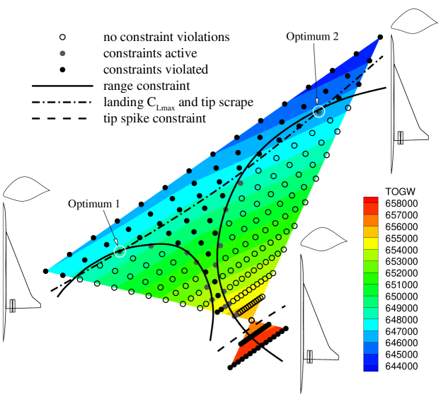
Figure 1: A pocket in an aircraft design space viewed as a slice through three design points [10] (courtesy Layne T. Watson).

The goal of this paper is to describe focused sampling strategies for mining scientific data. Our approach is based on the spatial aggregation language (SAL) [3], which supports construction of data interpretation and control design applications for spatially-distributed physical systems. Used as a basis for describing data mining algorithms, SAL programs also help exploit knowledge of physical properties such as continuity and locality in data fields. They work in a bottom-up manner to uncover regions of uniformity in spatially distributed data. In conjunction with this process, we introduce a top-down sampling strategy that focuses data collection in only those regions that are deemed most important to support a data mining objective. Together, they help define a methodology for mining in data-scarce domains. We describe this methodology at a high-level and devote the major part of the paper to two applications that employ it.

2 A Methodology for Mining in Data-Scarce Domains

It is possible to study the problem of sampling for targeted data mining activities, such as clustering, finding association rules, and decision tree construction [9]. This is the approach taken by work such as [12]. In this paper, however, we are interested in a general framework or language to express data mining operations on datasets and which can be used to study the design of data collection and sampling strategies. The spatial aggregation language (SAL) [3, 19] is such a framework.

2.1 SAL: The Spatial Aggregation Language

As a data mining framework, SAL is based on successive manipulations of data fields by a uniform vocabulary of aggregation, classification, and abstraction operators. Programming in SAL follows a philosophy of building a multi-layer hierarchy of aggregations of data. These increasingly abstract descriptions of data are built using explicit representations of physical knowledge, expressed as metrics, adjacency relations, and equivalence predicates. This allows a SAL program to uncover and exploit structures in physical data.

SAL programs employ what has been called an imagistic reasoning style [20]. They employ vision-like routines to manipulate multi-layer geometric and topological structures in spatially distributed data. SAL adopts a field ontology, in which the input is a field mapping from one continuum to another (e.g. 2-D temperature field: $\mathbb{R}^{2}\rightarrow\mathbb{R}^{1}$; 3-D fluid flow field: $\mathbb{R}^{3}\rightarrow\mathbb{R}^{3}$). Multi-layer structures arise from continuities in fields at multiple scales. Due to continuity, fields exhibit regions of uniformity, and these regions of uniformity can be abstracted as higher-level structures which in turn exhibit their own continuities. Task-specific domain knowledge specifies how to uncover such regions of uniformity, defining metrics for closeness of both field objects and their features. For example, isothermal contours are connected curves of nearby points with equal (or similar enough) temperature.

The identification of structures in a field is a form of data reduction: a relatively information-rich field representation is abstracted into a more concise structural representation (e.g. pressure data points into isobar curves or pressure cells; isobar curve segments into troughs). Navigating the mapping from field to abstract description through multiple layers rather than in one giant step allows the construction of more modular programs with more manageable pieces that can use similar processing techniques at different levels of abstraction. The multi-level mapping also allows higher-level layers to use global properties of lower-level objects as local properties of the higher-level objects. For example, the average temperature in a region is a global property when considered with respect to the temperature data points, but a local property when considered with respect to a more abstract region description. As this paper demonstrates, analysis of higher-level structures in such a hierarchy can guide interpretation of lower-level data.

Figure 2: SAL multi-layer spatial aggregates, uncovered by a uniform vocabulary of operators utilizing domain knowledge. A variety of scientific data mining tasks, such as vector field bundling, contour aggregation, correspondence abstraction, clustering, and uncovering regions of uniformity can be expressed as multi-level computations with SAL aggregates.

(a)	(b)	(c)	(d)
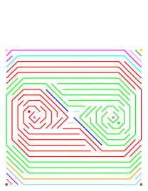
(e)	(f)	(g)	(h)

Figure 3: Example steps in SAL implementation of vector field analysis application. (a) Input vector field. (b) 8-adjacency neighborhood graph. (c) Forward neighbors. (d) Best forward neighbors. (e) Ngraph transposed from best forward neighbors. (f) Best backward neighbors. (g) Resulting adjacencies redescribed as curves. (h) Higher-level aggregation and classification of curves whose flows converge.

// (a) Read vector field. vect_field = read_point_point_field(infile); points = domain_space(vect_field); // (b) Aggregate with 8-adjacency (i.e. within 1.5 units). point_ngraph = aggregate(points, make_ngraph_near(1.5)); // (c) Compare vector directions with node-neighbor direction. angle = function (p1, p2) { dot(normalize(mean(feature(vect_field, p1), feature(vect_field, p2))), normalize(subtract(p2, p1))) } forward_ngraph = filter_ngraph(adj in point_ngraph, { angle(from(adj), to(adj)) > angle_similarity }) // (d) Find best forward neighbor, comparing vector direction // with ngraph edge direction and penalizing for distance. forward_metric = function (adj) { angle(from(adj), to(adj)) - distance_penalty * distance(from(adj),to(adj)) } best_forward_ngraph = best_neighbors_ngraph(forward_ngraph, forward_metric); // (e) Find backward neighbors by transposing best forward neighbors. backward_ngraph = transpose_ngraph(best_forward_ngraph); // (f) At junctions, keep best backward neighbor using metric // similar to that for best forward neighbors. backward_metric = function (adj) { angle(to(adj), from(adj)) - distance_penalty*distance(from(adj),to(adj)) } best_backward_ngraph = best_neighbors_ngraph(backward_ngraph, backward_metric); // (g) Move to a higher abstraction level by forming equivalence classes // from remaining groups and redescribing them as curves. final_ngraph = symmetric_ngraph(best_backward_ngraph, extend=true); point_classes = classify(points, make_classifier_transitive(final_ngraph)); points_to_curves = redescribe(classes(point_classes), make_redescribe_op_path_nline(final_ngraph)); trajs = high_level_objects(points_to_curves);

Figure 4: SAL data mining program for the vector field analysis application of Fig. 3.

SAL supports structure discovery through a small set of generic operators, parameterized with domain-specific knowledge, on uniform data types. These operators and data types mediate increasingly abstract descriptions of the input data (see Fig. 2) to form higher-level abstractions and mine patterns. The primitives in SAL are contiguous regions of space called spatial objects; the compounds are (possibly structured) collections of spatial objects; the abstraction mechanisms connect collections at one level of abstraction with single objects at a higher level.

SAL is currently available as a C++ library providing access to a large set of data type implementations and operations. In addition, an interpreted, interaction environment layered over the library supports rapid prototyping of data mining applications. It allows users to inspect data and structures, test the effects of different predicates, and graphically interact with representations of the structures.

To illustrate SAL programming style, consider the task of bundling vectors in a given vector field (e.g. wind velocity or temperature gradient) into a set of streamlines (paths through the field following the vector directions). This process can be depicted as shown in Fig. 3 and the corresponding SAL data mining program is shown in Fig. 4. The steps in this program are as follows: (a) Establish a field mapping points (locations) to points (vector directions, assumed here to be normalized). (b) Localize computation with a neighborhood graph, so that only spatially proximate points are compared. (c)–(f) Use a series of local computations on this representation to find equivalence classes of neighboring vectors with respect to vector direction (systematically eliminate all edges but those whose directions best match the vector direction at both endpoints). (g) Redescribe equivalence classes of vectors into more abstract streamline curves. (h) Aggregate and classify these curves into groups with similar flow behavior, using the exact same operators but with different metrics (code not shown). As this example illustrates, SAL provides a vocabulary for expressing the knowledge required (e.g., distance metrics and similarity metrics) for uncovering multi-level structures in spatial datasets. It has been applied to applications ranging from decentralized control design [2] to analysis of diffusion-reaction morphogenesis [16].

2.2 Data Collection and Sampling

The above example illustrated the use of SAL in a data-rich domain. The exploitation of physical properties is a central tenet of SAL since it drives the computation of multi-level spatial aggregates. Many important physical properties can be expressed as SAL computations by suitably defining adjacency relations and aggregation metrics. To extend the use of SAL to data-scarce settings, we present the sampling methodology outlined in Fig. 5.

Once again, it is easy to understand the methodology in the context of the vector-field bundling application (Fig. 3). Assume that we apply the SAL data mining program of Fig. 4 with a small dataset and have navigated upto the highest level of the hierarchy (streamlines bundled with convergent flows). The SAL program computes different streamline aggregations from a neighborhood graph and chooses one based on how well its curvature matches the direction of the vectors it aggregates. If data is scarce, it is likely that some of these classification decisions will be ambiguous, i.e., there may exist multiple streamline aggregations. In such a case, we would like to choose a new data sample that reduces the ambiguity and clarifies what the correct classification should be.

This is the essence of our sampling methodology: using SAL aggregates, we identify an information-theoretic measure (here, ambiguity) that can be used to drive stages of future data collection. For instance, the ambiguous streamline classifications can be summarized as a 2D ambiguity distribution that has a spike for every location where an ambiguity was detected. Reduction of ambiguity can be posed as the problem of minimization of (or maximization, as the case may be) a functional involving the (computed) ambiguity. The functional could be the entropy in the underlying data field, as revealed by the ambiguity distribution. Such a minimization will lead us to selecting a data point(s) that clarifies the distribution of streamlines, and hence makes more effective use of data for data mining purposes. The net effect of this methodology is that we are able to capture the desirability of a particular design (data layout) in terms of computations involving SAL aggregates. Thus, sampling is conducted for the express purpose of improving the quality and efficacy of data mining. The dataset is updated with the newly collected value and the process is repeated till a desired stopping criteria is met. For instance, we could terminate if the functional is within accepted bounds, or when there is no improvement in confidence of data mining results between successive rounds of data collection. In our case, when there is no further ambiguity.

This idea of sampling to satisfy particular design criteria has been studied in various contexts, especially spatial statistics [6, 11, 18]. Many of these approaches (including ours) rely on capturing properties of a desirable design in terms of a novel objective function. The distinguishing feature of our work is that it uses spatial information gleaned from a higher level of abstraction to focus data collection at the field/simulation code layer. The applications presented here are also novel in that they span and connect arbitrary levels of abstraction, thus suggesting new ways to integrate qualitative and quantitative simulation [4].

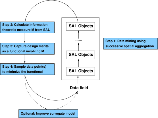
Figure 5: The sampling methodology for SAL mining in data-scarce domains.

We present concrete realizations of the above methodology in the next section. But before we proceed, it is pertinent to note an optional step in our methodology. The newly collected data value can be used to improve a surrogate model which then generates a dense data field for mining. A surrogate function is something that is used in lieu of the real data source, so as to generate sufficient data for mining purposes. This is often more advantageous than working directly with sparse data. Surrogate models are widely used in engineering design, optimization, and in response surface approximations [13, 15].

Together, SAL and our focused sampling methodology address the main issues raised in the beginning of the paper: SAL’s uniform use of fields and abstraction operators allows us to exploit prior knowledge in a bottom-up manner. Discrepancies as suggested by our knowledge of physical properties (e.g., ambiguities) are used in a top-down manner by the sampling methodology. Continuing these two stages alternatively leads to a closed-loop data mining solution for data-scarce domains.

3 Example Applications

3.1 Mining Pockets in Spatial Data

Our first application is motivated by the aircraft design problem and is meant to illustrate the basic idea of our methodology. Here, we are given a spatial vector field and we wish to identify pockets underlying the gradient. In a weather map, this might mean identifying pressure troughs, for instance. The question is: ‘where should data be collected so that we are able to mine the pockets with high confidence?’ We begin by presenting a mathematical function that gives rise to pockets in spatial fields. This function will be used to validate and test our data mining and sampling methodology.

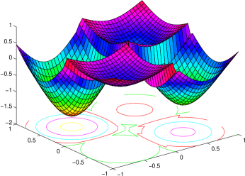
Figure 6: A 2D pocket function.

de Boor’s function

Carl de Boor invented a pocket function that exploits containment properties of the $n$-sphere of radius 1 centered at the origin ($\Sigma{x_{i}}^{2}\leq 1$) with respect to the $n$-dimensional hypercube defined by $x_{i}\in[-1,1],i=1\cdots n$. Even though the sphere is embedded inside the cube, notice that the ratio of the volume of the cube ($2^{n}$) to that of the sphere ($\pi^{n/2}/(n/2)!$) grows unboundedly with $n$. This means that the volume of a high-dimensional cube is concentrated in its corners (a counterintuitive notion at first). de Boor exploited this property to design a difficult-to-optimize function which assumes a pocket in each corner of the cube (Fig. 6), that is just outside the sphere. Formally, it can be defined as:

$$\alpha({\mathbf{X}}) = cos\left(\sum_{i=1}^{n}2^{i}\left(1+{x_{i}\over{\mid x_{i}\mid}}\right)\right)-2$$ (1)

$$\delta({\mathbf{X}}) = \|{\mathbf{X}}-0.5{\mathbf{I}}\|$$ (2)

$$p({\mathbf{X}}) = \alpha({\mathbf{X}})(1-\delta^{2}({\mathbf{X}})(3-2\delta({\mathbf{X}})))+1$$ (3)

where ${\mathbf{X}}$ is the n-dimensional point $(x_{1},x_{2},\cdots,x_{n})$ at which the pocket function $p$ is evaluated, ${\mathbf{I}}$ is the identity n-vector, and $\|\cdot\|$ is the $L_{2}$ norm.

It is easily seen that $p$ has $2^{n}$ pockets (local minima); if $n$ is large (say, 30, which means it will take more than half a million points to just represent the corners of the $n$-cube!), naive global optimization algorithms will require an unreasonable number of function evaluations to find the pockets. Our goal for data mining here is to obtain a qualitative indication of the existence, number, and locations of pockets, using low-fidelity models and/or as few data points as possible. The results can then be used to seed higher-fidelity calculations. This is also fundamentally different from DACE [18], polynomial response surface approximations [13], and other approaches in geo-statistics where the goal is accuracy of functional prediction at untested data points. Here, accuracy of estimation is traded for the ability to mine pockets.

Surrogate Function

In this study, we use the SAL vector-field bundling code presented earlier along with a surrogate model as the basis for generating a dense field of data. Surrogate theory is an established area in engineering optimization and there are several ways in which we can build a surrogate. However, the local nature of SAL computations means that we can be selective about our choice of surrogate representation. For example, global, least-squares type approximations are inappropriate since measurements at all locations are equally considered to uncover trends and patterns in a particular region. We advocate the use of kriging-type interpolators [18], which are local modeling methods with roots in Bayesian statistics. Kriging can handle situations with multiple local extrema (for example, in weather data, remote sensing data, etc.) and can easily exploit anisotropies and trends. Given $k$ observations, the interpolated model gives exact responses at these $k$ sites and estimates values at other sites by minimizing the mean squared error (MSE), assuming a random data process with zero mean and a known covariance function.

Formally (for two dimensions), the true function $p$ is assumed to be the realization of a random process such as:

$$p(x,y)=\beta+Z(x,y)$$ (4)

where $\beta$ is typically a uniform random variate, estimated based on the known $k$ values of $p$, and $Z$ is a correlation function. Kriging then estimates a model $p^{\prime}$ of the same form, based on the $k$ observations:

$$p^{\prime}(x_{i},y_{i})=E(p(x_{i},y_{i})\mathop{\,|\,}p(x_{1},y_{1}),\cdots,p(x_{k},y_{k}))$$ (5)

and minimizing mean squared error between $p^{\prime}$ and $p$:

$$MSE=E(p^{\prime}(x,y)-p(x,y))^{2}$$ (6)

A typical choice for $Z$ in $p^{\prime}$ is $\sigma^{2}R$, where scalar $\sigma^{2}$ is the estimated variance, and correlation matrix $R$ encodes domain-specific constraints and reflects the current fidelity of data. We use an exponential function for entries in $R$, with two parameters $C_{1}$ and $C_{2}$:

$$R_{ij}=e^{-C_{1}|x_{i}-x_{j}|^{2}-C_{2}|y_{i}-y_{j}|^{2}}$$ (7)

Intuitively, values at closer points should be more highly correlated.

The estimator minimizing mean squared error is then obtained by multi-dimensional optimization (the derivation from Eqs. 6 and 7 is beyond the scope of this paper):

$$\max_{C}{\frac{-k}{2}}(\ln\sigma^{2}+\ln|R|)$$ (8)

This expression satisfies the conditions that there is no error between the model and the true values at the chosen $k$ sites, and that all variability in the model arises from the design of $Z$. The multi-dimensional optimization is often performed by gradient descent or pattern search methods. More details are available in [18], which demonstrates this methodology in the context of the design and analysis of computer experiments.

Data Mining and Sampling Methodology

The bottom-up computation of SAL aggregates from the surrogate model’s outputs will possibly lead to some ambiguous streamline classifications, as discussed earlier. Ambiguity can reflect the desirability of acquiring data at or near a specified point, to clarify the correct classification and to serve as a mathematical criterion of information content. There are several ways in which we can use information about ambiguity to drive data collection. In this study, we express the ambiguities as a distribution describing the number of possible good neighbors (for a streamline). This ambiguity distribution provides a novel mechanism to include qualitative information — streamlines that agree will generally contribute less to data mining, for information purposes. The information-theoretic measure $M$ (ref. Fig. 5) was thus defined to be the ambiguity distribution $\wp$.

The functional was defined as the posterior entropy $E(-\log d)$, where $d$ is the conditional density of $\wp$ over the design space not covered by the current data values. By a reduction argument, minimizing this posterior entropy can be shown to be maximizing the prior entropy over the unsampled design space [18]. In turn, this means that the amount of information obtained from an experiment (additional data collection) is maximized. In addition, we also incorporated $\wp$ as an indicator covariance term in our surrogate model (this is a conventional method for including qualitative information in an interpolatory model [11]).

Experimental Results

The initial experimental configuration used a face-centered design ($4$ points in the 2D case). A surrogate model by kriging interpolation then generated data on a $41^{n}$-point grid. de Boor’s function was used as the source for data values; we also employed pseudorandom perturbations of it that shift the pockets from the corners in a somewhat unpredictable way (see [1] for details). In total, we experimented with 100 perturbed variations (each) of the 2D and 3D pocket functions. For each of these cases, data collection was organized in rounds of one extra sample each (that minimizes the above functional). The number of samples needed to mine all the pockets by SAL was recorded. We also compared our results with those obtained from a pure DACE/kriging approach (i.e., where sampling was directed at improving accuracy of function estimation). In other words, we used the DACE methodology to suggest new locations for data collection and determined how these choices fared with respect to mining the pockets.

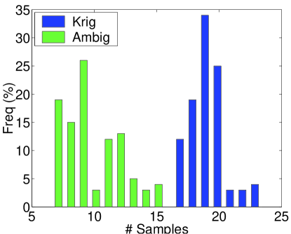
Figure 7: Pocket-finding results (2D) show that focused sampling using a measure of ambiguity always requires fewer total samples (7-15) than conventional kriging (17-23).

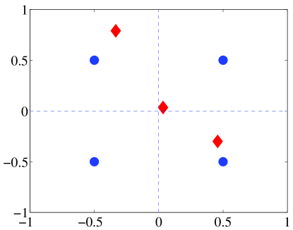
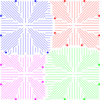
Figure 8: Mining pockets in 2D from only 7 sample points. (left) The chosen sample locations: 4 initial face-centered samples (marked as blue circles) plus 3 samples selected by our methodology (marked as red diamonds). Note that no additional sample is required in the lower-left quadrant. (right) SAL structures in surrogate model data, confirming the existence of four pockets.

Fig. 7 shows the distributions of total number of data samples required to mine the four pockets for the 2D case. We were thus able to mine the 2D pockets using 3 to 11 additional samples, whereas the conventional kriging approach required 13 to 19 additional samples. The results were were more striking in the 3D case: at most 42 additional samples for focused sampling and upto 151 points for conventional kriging. This shows that our focused sampling methodology performs 40-75% better than sampling by conventional kriging.

Fig. 8 (left) describes a 2D design involving only $7$ total data points that is able to mine the four pockets. Counterintuitively, no additional sample is required in the lower left quadrant! While this will lead to a highly sub-optimal design (from the traditional viewpoint of minimizing variance in predicted values), it is nevertheless an appropriate design for data mining purposes. In particular, this means that neighborhood calculations involving the other three quadrants are enough to uncover the pocket in the fourth quadrant. Since the kriging interpolator uses local modeling and since pockets in 2D effectively occupy the quadrants, obtaining measurements at ambiguous locations serves to capture the relatively narrow regime of each dip, which in turn helps to distinguish the pocket in the neighboring quadrant. This effect is hard to achieve without exploiting knowledge of physical properties, in this case, locality of the dips.

3.2 Qualitative Jordan Form Determination

In our second application, we use our methodology to identify the most probable Jordan form of a given matrix. This is a good application for data mining since the direct computation of the Jordan form leads to a numerically unstable algorithm.

Jordan forms

A matrix $\mathcal{A}$ (real or complex) that has $r$ independent eigenvectors has a Jordan form that consists of $r$ blocks. Each of these blocks is an upper triangular matrix that is associated with one of the eigenvectors of $\mathcal{A}$ and whose size describes the multiplicity of the corresponding eigenvalue. For the given matrix $\mathcal{A}$, the diagonalization thus posits a nonsingular matrix $\mathcal{B}$ such that:

$$\mathcal{B}^{-1}\mathcal{A}\mathcal{B}=\left[\begin{array}[]{cccc}{\mathcal{J}}_{1}&&&\\ &{\mathcal{J}}_{2}&&\\ &&\cdot&\\ &&&{\mathcal{J}}_{r}\\ \end{array}\right]$$ (9)

where

$${\mathcal{J}}_{i}=\left[\begin{array}[]{cccc}\lambda_{i}&1&&\\ &\cdot&1&\\ &&\cdot&1\\ &&&\lambda_{i}\\ \end{array}\right]$$ (10)

and $\lambda_{i}$ is the eigenvalue revealed by the $i$th Jordan block ($\mathcal{J}_{i}$). The Jordan form is most easily explained by looking at how eigenvectors are distributed for a given eigenvalue. Consider, for example, the matrix

$$\left[\begin{array}[]{crr}1&1&-1\\ 0&0&2\\ 0&-1&3\\ \end{array}\right]$$

that has eigenvalues at 1, 1, and 2. This matrix has only two eigenvectors, as revealed by the two-block structure of its Jordan form:

$$\left[\begin{array}[]{cr|r}1&1&0\\ 0&1&0\\ \hline\cr 0&0&2\\ \end{array}\right]$$

The Jordan form is unique modulo shufflings of the blocks and, in this case, shows that there is one eigenvalue ($1$) of multiplicity $2$ and one eigenvalue ($2$) of multiplicty $1$. We say that the matrix has the Jordan structure given by $(1)^{2}(2)^{1}$. In contrast, the matrix

$$\left[\begin{array}[]{crr}1&0&0\\ 0&2&0\\ 0&0&1\\ \end{array}\right]$$

has the same eigenvalues but a three-block Jordan structure:

$$\left[\begin{array}[]{c|r|r}1&0&0\\ \hline\cr 0&1&0\\ \hline\cr 0&0&2\\ \end{array}\right]$$

This is because there are three independent eigenvectors (the unit vectors, actually). The diagonalizing matrix is thus the identity matrix and the Jordan form has three permutations. The Jordan structure is therefore given by $(1)^{1}(1)^{1}(2)^{1}$. These two examples show that a given eigenvalue’s multiplicity could be distributed across one, many, or all Jordan blocks. Correlating the eigenvalue with the block structure is an important problem in numerical analysis.

The typical approach to computing the Jordan form is to ‘follow the staircase’ pattern of the structure and perform rank determinations in conjunction with ascertaining the eigenvalues. One of the more serious caveats with such an approach involves mistaking an eigenvalue of multiplicity $>1$ for multiple eigenvalues [8]. In the first example matrix above, this might lead to inferring that the Jordan form has three blocks. The extra care needed to safeguard staircase algorithms usually involves more complexity than the original computation to be performed! The ill-conditioned nature of this computation has thus traditionally prompted numerical analysts to favor other, more stable, decompositions.

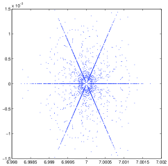
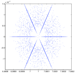
Figure 9: Superimposed spectra for assessing the Jordan form of the Brunet matrix. Two Jordan blocks of multiplicity 3 are observed for eigenvalue 7, at different (left, right) perturbation levels.

Qualitative assessment of Jordan forms

A recent development has been the acceptance of a qualitative approach to Jordan structure determination, proposed by Chaitin-Chatelin and Frayssé [5]. This approach does not employ the staircase idea and, instead, exploits a semantics of eigenvalue perturbations to infer multiplicity. This leads to a geometrically intuitive algorithm that can be implemented using SAL.

Consider a matrix that has eigenvalues $\lambda_{1},\lambda_{2},\cdots,\lambda_{n}$ with multiplicities $\rho_{1},\rho_{2},\cdots,\rho_{n}$ (resp). Any attempt at finding the eigenvalues (e.g., determining the roots of the characteristic polynomial) is intrinsically subject to the numerical analysis dogma: the problem being solved will actually be a perturbed version of the original problem. This allows the expression of the computed eigenvalues in terms of perturbations on the actual eigenvalues. It can be easily seen that the computed eigenvalue corresponding to any $\lambda_{k}$ will be distributed on the complex plane as:

$$\lambda_{k}+|\Delta|^{1\over{\rho_{k}}}e^{{i\phi}\over{\rho_{k}}}$$

where the phase $\phi$ of the perturbation $\Delta$ ranges over {$2\pi,4\pi,\ldots,2\rho_{k}\pi$} if $\Delta$ is positive and over {$3\pi,5\pi,\ldots,2(\rho_{k}+1)\pi$} if $\Delta$ is negative. The insight in [5] is to superimpose numerous such perturbed calculations graphically so that the aggregate picture reveals the $\rho_{k}$ of the eigenvalue $\lambda_{k}$. Notice that the phase variations imply that the computed eigenvalues will be lying on the vertices of a regular polygon centered on the actual eigenvalue and where the number of sides is two times the multiplicity of the considered eigenvalue (this takes into account both positive and negative $\Delta$). Since the diameter of the polygon is influenced by $\Delta$, iterating this process over many $\Delta$ will lead to a ‘sticks’ depiction of the Jordan form.

To illustrate, we choose a matrix whose computations will be more prone to finite precision errors. Perturbations on the 8-by-8 Brunet matrix [5] with Jordan structure $(-1)^{1}(-2)^{1}(7)^{3}(7)^{3}$ induce the superimposed structures shown in Fig. 9. The left part of Fig. 9 depicts normwise relative perturbations in the scale of $[2^{-50},2^{-40}]$. The six sticks around the eigenvalue at 7 clearly reveal that its Jordan block is of size 3. The other Jordan block, also centered at 7, is revealed if we conduct our exploration at a finer perturbation level. Fig. 9 reveals the second Jordan block using perturbations in the range $[2^{-53},2^{-50}]$. The noise in both pictures is a consequence of (i) having two Jordan blocks with the same size, and (ii) a ‘ring’ phenomenon studied in [7]; we do not attempt to capture these effects in this paper.

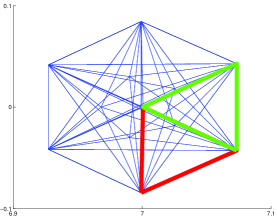
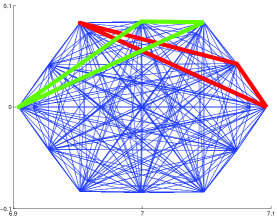
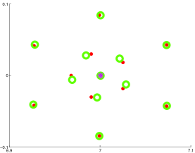
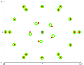
Figure 10: Mining Jordan forms from (left) a small sample set, and (right) large sample set. (top) Approximately congruent triangles. (bottom) Evaluation of correspondence of rotated triangles in terms of match between original (red dots) and rotated (green circles) samples.

Data Mining and Sampling Methodology

For this study, we collect data by random normwise perturbations in a given region and a SAL program determines multiplicity by detecting symmetry correspondence in the samples. The first aggregation level collects the samples for a given perturbation into triangles. The second aggregation level finds congruent triangles via geometric hashing [14], and uses congruence to establish an analogy relation among triangle vertices. This relation is then abstracted into a rotation about a point (the eigenvalue), and evaluated for whether each point rotates onto another and whether matches define regular polygons. A third level then compares rotations across different perturbations, re-visiting perturbations or choosing new perturbations in order to disambiguate (see Fig. 10). The end result of this analysis is a confidence measure on models of possible Jordan forms. Each model is defined by its estimate of $\lambda$ and $\rho$ (notice that we are working only within one region at a time). The measure $M$ was defined to be the joint probability distribution over the space of $\lambda$ and $\rho$.

Experimental Results

Since our Jordan form computation treats multiple perturbations (irresp. of level) as independent estimates of eigenstructure, the idea of sampling here is not ‘where to collect,’ but ‘how much to collect.’ The goal of data mining is hence to improve our confidence in model evaluation. We organized data collection into rounds of 6-8 samples each, varied a tolerance parameter for triangle congruence from 0.1 to 0.5 (effectively increasing the number of models posited), and determined the number of rounds needed to determine the Jordan form. As test cases, we used the set of matrices studied in [5]. On average, our focused sampling approach required 1 round of data collection at a tolerance of 0.1 and up to 2.7 rounds at 0.5. Even with a large number of models posited, additional data quickly weeded out bad models. Fig. 10 demonstrates this mechanism on the Brunet matrix discussed above for two sets of sample points. To the best of our knowledge, this is the only known known focused sampling methodology for this domain; we hence are unable to present any comparisons. However, it is clear that by harnessing domain knowledge about correspondences, we have arrived at an intelligent sampling methodology that resembles what a human would obtain by visual inspection.

4 Discussion

The presented methodology for mining in data-scarce domains has several intrinsic benefits. First, it is based on a uniform vocabulary of operators that can be exploited for a rich diversity of applications. Second, it demonstrates a novel factorization to the problem of mining when data is scarce, namely, formulating an experiment design methodology to clarify, disambiguate, and improve confidences in higher-level aggregates of data. This allows us to bridge qualitative and quantitative information in a unified framework. SAL programs thus uncover bottom-up structures in data systematically and use difficulties encountered in this process (ambiguities, lack of correspondences) to guide top-down selection of additional data samples. By using knowledge of physical properties explicitly, our approach can provide more holistic and explainable results than off-the-shelf data mining algorithms. Third, our methodology can co-exist with more traditional approaches to problem solving (numerical analysis, optimization) and is not meant to be a replacement or a contrasting approach. This is amply demonstrated in each of the two applications above, where connections with various traditional methodologies have been carefully established.

The methodology makes several intrinsic assumptions which we only briefly mention here. All of our applications have been such that the cause, formation, and effect of the relevant physical properties are well understood. This is precisely what allows us to act decisively based on higher-level information from SAL aggregates, through the measure $M$. It also assumes that the problems that will be encountered by the mining algorithm are the same as the problems for which it was designed. This is an inheritance from Bayesian inductive inference and leads to fundamental limitations on what can be done in such a setting. For instance, if new data does not help clarify an ambiguity, does the fault lie with the model (SAL higher-level aggregate) or with the data? We can summarize this problem by saying that the approach requires strong a priori information about what is possible and what is not.

Nevertheless, by advocating targeted use of domain specific knowledge and aiding qualitative model selection, our methodology is more efficient at determining high level models from empirical data. Together, SAL and our information-theoretic measure $M$ encapsulate knowledge about physical properties and this is what makes our methodology a viable one for data mining purposes. In future we aim to characterize more formally the particular forms of domain knowledge that help overcome sparsity and noise in scientific datasets.

It should be mentioned that while the two studies formulate their sampling objectives differently, they are naturally supported by the SAL framework:

• (pockets) Where should I collect data in order to mine the pockets with high confidence?

• (Jordan forms) How much data should I collect in order to determine the right Jordan form with high confidence?

One could imagine extending our framework to also take into account the expense of data samples. If the cost of data collection is non-uniform across the domain, then including this in the design of our functional will allow us to tradeoff the cost of gathering information with the expected improvement in problem solving performance. This area of data mining is referred to as active learning.

Data mining can sometimes be a controversial term in a discipline that is used to mathematical rigor; this is because it often used synonymously with ‘lack of a hypothesis or theory.’ We hope to have convinced the reader that this need not be the case and that data mining can indeed be sensitive to knowledge about the domain, especially physical properties of the kind we have harnessed here. As data mining applications become more prevalent in science, the need to incorporate a priori domain knowledge will only become more important.

References

- [1] C. Bailey-Kellogg and N. Ramakrishnan. Ambiguity-Directed Sampling for Qualitative Analysis of Sparse Data from Spatially Distributed Physical Systems. In Proceedings of the Seventeenth International Joint Conference on Artificial Intelligence (IJCAI-01), pages 43–50, 2001.
- [2] C. Bailey-Kellogg and F. Zhao. Influence-Based Model Decomposition for Reasoning about Spatially Distributed Physical Systems. Artificial Intelligence, Vol. 130(2):pages 125–166, 2001.
- [3] C. Bailey-Kellogg, F. Zhao, and K. Yip. Spatial Aggregation: Language and Applications. In Proceedings of the Thirteenth National Conference on Artificial Intelligence (AAAI’96), pages 517–522, 1996.
- [4] D. Berleant and B. Kuipers. Qualitative and Quantitative Simulation: Bridging the Gap. Artificial Intelligence, Vol. 95(2):pages 215–255, 1998.
- [5] F. Chaitin-Chatelin and V. Frayssé. Lectures on Finite Precision Computations. SIAM Monographs, 1996.
- [6] R.G. Easterling. Comment on ‘Design and Analysis of Computer Experiments’. Statistical Science, Vol. 4(4):pages 425–427, 1989.
- [7] A. Edelman and Y. Ma. Non-Generic Eigenvalue Perturbations of Jordan Blocks. Linear Algebra & Applications, Vol. 273(1-3):pages 45–63, 1998.
- [8] A. Edelman and Y. Ma. Staircase Failures Explained by Orthogonal Versal Forms. SIAM Journal on Matrix Analysis and Applications, Vol. 21(3):pages 1004–1025, 2000.
- [9] V. Ganti, J. Gehrke, and R. Ramakrishnan. Mining Very Large Databases. IEEE Computer, Vol. 32(8):pages 38–45, August 1999.
- [10] A. Goel, C.A. Baker, C.A. Shaffer, B. Grossman, W.H. Mason, L.T. Watson, and R.T. Haftka. VizCraft: A Problem-Solving Environment for Aircraft Configuration Design. IEEE/AIP Computing in Science and Engineering, Vol. 3(1):pages 56–66, 2001.
- [11] A. Journel. Constrainted Interpolation and Qualitative Information - The Soft Kriging Approach. Mathematical Geology, Vol. 18(2):pages 269–286, November 1986.
- [12] J. Kivinen and H. Mannila. The Use of Sampling in Knowledge Discovery. In Proceedings of the Thirteenth ACM Symposium on Principles of Database Systems, pages 77–85, 1994.
- [13] D.L. Knill, A.A. Giunta, C.A. Baker, B. Grossman, W.H. Mason, R.T. Haftka, and L.T. Watson. Response Surface Models Combining Linear and Euler Aerodynamics for Supersonic Transport Design. Journal of Aircraft, 36(1):pages 75–86, 1999.
- [14] Y. Lamdan and H. Wolfson. Geometric Hashing: A General and Efficient Model-Based Recognition Scheme. In Proceedings of the Second International Conference on Computer Vision (ICCV), pages 238–249, 1988.
- [15] R.H. Myers and D.C. Montgomery. Response Surface Methodology: Process and Product Optimization using Designed Experiments. Wiley, Jan 2002.
- [16] I. Ordóñez and F. Zhao. STA: Spatio-Temporal Aggregation with Applications to Analysis of Diffusion-Reaction Phenomena. In Proceedings of the Seventeenth National Conference on Artificial Intelligence (AAAI’00), pages 517–523, 2000.
- [17] N. Ramakrishnan and A.Y. Grama. Mining Scientific Data. Advances in Computers, Vol. 55:pages 119–169, Sep 2001.
- [18] J. Sacks, W.J. Welch, T.J. Mitchell, and H.P. Wynn. Design and Analysis of Computer Experiments. Statistical Science, Vol. 4(4):pages 409–435, 1989.
- [19] K.M. Yip and F. Zhao. Spatial Aggregation: Theory and Applications. Journal of Artificial Intelligence Research, Vol. 5:pages 1–26, 1996.
- [20] K.M. Yip, F. Zhao, and E. Sacks. Imagistic Reasoning. ACM Computing Surveys, Vol. 27(3):pages 363–365, 1995.