Learning from Scarce Experience

Abstract

Searching the space of policies directly for the optimal policy has been one popular method for solving partially observable reinforcement learning problems. Typically, with each change of the target policy, its value is estimated from the results of following that very policy. This requires a large number of interactions with the environment as different polices are considered. We present a family of algorithms based on likelihood ratio estimation that use data gathered when executing one policy (or collection of policies) to estimate the value of a different policy. The algorithms combine estimation and optimization stages. The former utilizes experience to build a non-parametric representation of an optimized function. The latter performs optimization on this estimate. We show positive empirical results and provide the sample complexity bound.

1 Introduction

Research in reinforcement learning focuses on designing algorithms for an agent interacting with an environment to adjust its behavior to optimize a long-term return. For environments which are fully-observable (i.e. the observations the agent makes contain all of the necessary information about the state of the environment), this problem can often be solved using a one-step look ahead analysis to formulate the solution as a dynamic programming problem. However, for the case of partially observable domains (i.e. the observations are stochastic or incomplete representations of the environment’s state), the perceptual aliasing of the observations makes such methods infeasible.

One viable approach is to search directly in a parameterized space of policies for a local optimum. Following Williams’s reinforce algorithm (Williams92), searching by gradient descent has been considered for a variety of policy classes (Marbach; Baird99; MeuleauUAI99; SuttonNIPS99; BaxterICML00). A commonly recognized shortcoming of all these variations on gradient descent policy search is that they require a very large number of samples (instances of agent-environment interaction) to converge.

This inefficiency arises because the value of the policy (or its derivative) is estimated by sampling from the returns obtained by following that same policy. Thus, after one policy is evaluated and a new one proposed, the samples taken from the old policy must be discarded. Each new step of the policy search algorithm requires a new set of samples. The key to solving this inefficiency is to use data gathered when using one policy to estimate the value of another policy. The method known as “likelihood ratio” estimation enables this data reuse.

Stochastic gradient methods and likelihood ratios have been long used for optimization problems (see work of (?; ?; ?; ?)). Recently, stochastic gradient descent methods, in particular reinforce (Williams92; Williams91), have been used in conjunction with policy classes constrained in various ways: with external memory (Peshkin99), finite state controllers (MeuleauUAI99) and in multi-agent settings (Peshkin00). The idea of using likelihood ratios in reinforcement learning was suggested by ? (?) and developed for solving mdps with function approximation by ? (?) and for gradient descent in finite state controllers by ? (?). However, only on-line optimization was considered. (?; ?) developed greedy algorithm for combining samples from multiple policies in normalized estimators and demonstrated a dramatic improvement in performance. ? (?) showed that likelihood-ratio estimation enables the application of methods from statistical learning theory to derive pac bounds on sample complexity.

? (?) provide a method for estimating the return of every policy simultaneously using data gathered while executing a fixed policy without the use of likelihood ratios. In some domains, there is a natural distance between observations and actions which also allows one to re-use experience without likelihood ratio estimation. ? (?) demonstrate algorithms for kernel-based rl in one such domain: financial planing and investments.

This paper extends our previous work by presenting a generalized method of using likelihood ratio estimation in policy search and investigating the performance of this method under different conditions on illustrative examples. By this publication we hope to stimulate a dialog between the communities of reinforcement learning and computational learning theory. We present a clear outline of all algorithms in a hope to attract wider research community to applying these algorithms in various domains. We also present some new bounds on a sample complexity of these algorithms, making an attempt to relate these results to empirical results. We begin this paper with a brief definition of reinforcement learning and sampling in order to clarify our notation. Then we present our algorithm and consider the question of how to sample. Finally we consider the question of how much to sample and present a pac-style bound as a quantitative answer.

2 Background

We introduce the environment model and importance sampling in a single mathematical notation. In particular, we keep the standard notation for partially observable Markov decision processes and modify the sampling notation to be consistent.

2.1 Environment Model

The class of problems we consider can be described by the partially observable Markov decision process (pomdp) model. In a pomdp, a sequence of events occur for each time step: an agent observes the observation $o(t)\in{\cal O}$ dependent on the state of environment $s(t)\in{\cal S}$; it performs an action $a(t)\in{\cal A}$ according to its policy, inducing a state transition of the environment; then it receives a reward $r(t)$ based on the action taken and the environment’s state. A pomdp is defined by four probability distributions (and the spaces over which those distributions are defined): a distribution over starting states, a distribution over observations conditioned on the state, a distribution over next states conditioned on the current state and the agent’s action, and a distribution over rewards given the state and action. These distributions, specifying the dynamics of the environment, are unknown to the agent along with the state space of process, ${\cal S}$.

Let $H=\left\{\langle o(1),a(1),r(1),\ldots,o(t),a(t),r(t),o(t+1)\rangle\right\}$ denote the set of all possible experiences sequences of length $t$. Generally speaking, in a pomdp, a policy $\pi$ is a function specifying the action to perform at each time step as a function of the whole previous history: $\pi:H\rightarrow{\cal P}(A)$. This function is parameterized by a vector $\theta\in\Theta$. Policy class $\Theta$ is a set of policies realizable by all parameter settings. We assume that the probability of the elementary event is bounded away from zero: $0\leq\underline{c}<\Pr(a|h,\theta)<\overline{c}\leq 1$, for any $a\!\in\!A$, $h\!\in\!H$, and $\theta\!\in\!\Theta$. A history $h$ includes several immediate rewards $\langle r(1),\ldots,r(i),\ldots\rangle$ that are typically summed to form a return, $R(h)$, but our results are independent of the method used to compute the return.

Together with the distributions defined by the pomdp, any policy $\theta\in\Theta$ defines a conditional distribution $\Pr(h|\theta)$ on the class of all histories $H$. The value of policy $\theta$ is the expected return according to the probability induced by this policy on the history space: $V(\theta)\!=\!{\rm E}_{\theta}\left[R(h)\right]=\sum_{h\in H}\left[R(h)\Pr(h|\theta)\right],$ where ${\rm E}_{\theta}$ stands for ${\rm E}_{\Pr(h|\theta)}$. We assume that policy values (and returns) are non-negative and bounded by $V_{max}$. The objective of the agent is to find a policy $\theta^{*}$ with optimal value: $\theta^{*}={\rm argmax}_{\theta}V(\theta)$. Because the agent does not have a model of the environment’s dynamics or reward function, it can not calculate $\Pr(h|\theta)$ and must estimate it via sampling.

2.2 Sampling

If we wish to estimate the value $V(\theta)$ of the policy $\theta$, we may draw sample histories from the distribution induced by this policy by executing the policy multiple times in the environment. After taking $N$ samples $\bar{h}=\{h_{i}\},i\in(1,\dots,N)$ we can use the unbiased estimator:

$$\hat{V}_{\bar{h}}(\theta)=\frac{1}{N}\sum_{i}R(h_{i})\,\,.$$

Imagine, however, that we are unable to sample from the policy $\theta$ directly, but instead have samples from another policy $\theta^{\prime}$. The intuition is that if we knew how “similar” those two policies were to one another, we could use samples drawn according to the distribution $\theta^{\prime}$ and make an adjustment proportional to the similarity of the policies. Formally we have:
$V(\theta)=\sum_{h}R(h)\Pr(h|\theta)=\sum_{h}R(h)\frac{\Pr(h|\theta^{\prime})}{\Pr(h|\theta^{\prime})}\Pr(h|\theta)$
      $=\sum_{h}R(h)\frac{\Pr(h|\theta)}{\Pr(h|\theta^{\prime})}\Pr(h|\theta^{\prime})={\rm E}_{\theta^{\prime}}\left[R(h)\frac{\Pr(h|\theta)}{\Pr(h|\theta^{\prime})}\right]\;.$
Now we can construct an unbiased indirect estimator for the distribution $\Pr(h|\theta^{\prime})$ which is called an importance sampling estimator (Rubinstein81) $\hat{V}^{\rm IS}_{\theta^{\prime},\bar{h}}(\theta)$ of $V(\theta)$:

$$\hat{V}^{\rm IS}_{\theta^{\prime},\bar{h}}(\theta)=\frac{1}{N}\sum_{i}R(h_{i})\frac{\Pr(h_{i}|\theta)}{\Pr(h_{i}|\theta^{\prime})}\,\,.$$

We can normalize the importance sampling estimate to obtain a lower variance estimate at the cost of adding bias. Such an estimator is called a weighted importance sampling estimator and has the form

$$\hat{V}^{\rm WIS}_{\theta^{\prime},\bar{h}}(\theta)=\frac{1}{\sum_{i}\frac{\Pr(h_{i}|\theta)}{\Pr(h_{i}|\theta^{\prime})}}\sum_{i}R(h_{i})\frac{\Pr(h_{i}|\theta)}{\Pr(h_{i}|\theta^{\prime})}\,,$$

which has been found to be better-behaved than $V^{\rm IS}_{\theta^{\prime},\bar{h}}(\theta)$ both theoretically and empirically (MeuleauTR00; Shelton01; PrecupICML00).

Note that both estimators contain the quantity $\frac{\Pr(h_{i}|\theta)}{\Pr(h_{i}|\theta^{\prime})}$, a ratio of likelihoods. The key observation for the remainder of this paper is that while an agent is not assumed to have a model of the environment and therefore is not able to calculate $\Pr(h|\theta)$, it is able to calculate the likelihood ratio $\frac{\Pr(h|\theta)}{\Pr(h|{\theta^{\prime}})}$ for any two policies $\theta$ and $\theta^{\prime}$ (SutBar98; MeuleauTR00; PeshkinPhD). $\Pr(h|\theta)$ can be written as a product of $\Phi(h)$ and $\Psi(h)$ where $\Phi(h)=\prod_{t=1}^{T}\Pr(a(t)|o(1),\dots,o(t),\theta)$ is the contribution of all of the agent’s actions to the likelihood of the history, and $\Psi(h)$ is the contribution of environmental events. Because the $\Psi(h)$ component is independent of the policy (i.e. it does not depend on the policy parameter, only on the history and the pomdp distributions), it cancels from the ratio, and we have $\frac{\Pr(h|\theta)}{\Pr(h|{\theta^{\prime}})}=\frac{\Phi(h|\theta)}{\Phi(h|{\theta^{\prime}})}$. $\Phi(h|\theta)$ depends only on the agent, the observations, and the actions (not the states), is known to the agent, and can be computed and differentiated. This allows us to construct more efficient learning algorithms that can take advantage of past experience.

Finally, if the sampling distribution is not constant (i.e. each sample is drawn from a different distribution), a single unbiased importance sampling estimator can be constructed by using all of the samples where the assumed single sampling distribution is the mixture of the true sampling distributions. Thus, if samples were taken according to policies $\theta_{1},\theta_{2},\dots,\theta_{n}$, $\Pr(h|{\theta^{\prime}})$ from above is replaced with $\frac{1}{N}\sum_{j}\Pr(h|{\theta_{j}})$. ? (?) gives more details for importance sampling estimators with independent, but not identically drawn, samples. Using this new estimator allows us to change policies (sampling distributions) during sampling.

3 Algorithms

Consider constructing a proxy environment that contains a non-parametric model of the values of all policies as illustrated by Figure 1. This model is a result of trying several policies $\theta_{1}\ldots\theta_{N}$. Given an arbitrary new policy $\theta\in\Theta$, the proxy environment returns an estimate of its value $\hat{V}(\theta)$ as if the policy were tried in the real environment. Assuming that obtaining a sample from environment is costly, we want to construct the proxy module based only on a small number of queries about policies $\{\theta_{i}\},i=1\dots N$ that return values $R_{i}$. These queries are implemented by the sample routine (Table 1). After getting $N$ samples, it requires memory of size $O(NT(\log|{\cal O}|+\log|{\cal A}|))$ to store the data, where $T$ is the length of a trial and ${\cal O}$ and ${\cal A}$ are the sets of possible observations and action respectively. However, for many policy classes this memory requirement can be reduced. For example, if the policy class is reactive (conditioned on the current observation, the probability of the current action has no dependence on the past), the history can be summarized sufficiently by the counts of the number of times each action was chosen after each observation. This requires memory of size $O(N\log(T)|{\cal O}||{\cal A}|)$.

Figure 1: A diagram of the policy evaluation process. The sampling process is costly and therefore only performed a limited number of times. The proxy collects the samples from the environment and constructs an agent-centric model that predicts the effects of hypothetical agent policies. The agent learns by interacting with the proxy.

Table 1: The sample routine accepts a policy parameter setting and outputs the return and history from one sample of the policy. Note that in many cases the entire history need not be returned.

 

Input: policy $\theta$
Init:
	$h\leftarrow(),R\leftarrow 0$
	Get initial observation $o_{0}$.
For each time step $t$ of the trial:
	Draw next $a_{t}$ from $\pi(o_{t},a_{t},\bar{\theta})$
	Execute $a_{t}$.
	Get observation $o_{t}$, reward $r_{t}$.
	$R\leftarrow R+r_{t}$
	$\text{\tt concatenate}(h,(o_{t},a_{t}))$
Output: experience $\langle R,h\rangle$

 

Table 2: The evaluate routine computes the proxy’s estimate of the value of a policy and its derivative. The inner loop (over $j$) can be removed with caching, making the routine faster.

 

Input: policy $\theta$, data $D=\{\langle\theta_{i},R_{i},h_{i}\rangle\}\ \mbox{for}\ i\in\{1\dots N\}$
Init: $\hat{V}\leftarrow 0$, $\Delta\hat{V}\leftarrow 0$, $\kappa\leftarrow 0$
For $i=1$ to $N$:
	Init: $\Psi_{i}^{\prime}\leftarrow 0$
	For $j=1$ to $N$:
		$\Phi_{i}^{\prime}\leftarrow\Phi_{i}^{\prime}+\Phi(h_{i}|\theta_{j})$
	$\Phi_{i}\leftarrow\Phi(h_{i}|\theta)$
	$\kappa\leftarrow\kappa+\frac{\Phi_{i}}{\Phi_{i}^{\prime}}$
For $i=1$ to $N$:
	$\hat{V}\leftarrow\hat{V}+R_{i}\frac{\Phi_{i}}{\Phi_{i}^{\prime}}$
$\hat{V}\leftarrow\frac{\hat{V}}{\kappa}$
For $i=1$ to $N$:
	$\Delta\Phi_{i}\leftarrow\frac{\partial\Phi(h_{i}|\theta)}{\partial\theta}$
	$\Delta\hat{V}\leftarrow\Delta\hat{V}+(R_{i}-\hat{V})\frac{\Delta\Phi_{i}}{\Phi_{i}^{\prime}}$
$\Delta\hat{V}\leftarrow\frac{\Delta\hat{V}}{\kappa}$
Output: proxy evaluation $\hat{V}$ and derivative $\Delta\hat{V}$

 

This proxy can be queried by the learning algorithm as shown in table 2. In response to a policy parameter settings, the routine evaluate returns its estimate of the expected return and its derivative. The algorithm shown in table 2 computes the weighted importance sampling estimate. For simplicity, the inner loop (over $j$) is shown. In practice the computations in this loop do not need to be redone for every evaluation. Using memory of size $O(N)$, the values $\Phi^{\prime}_{i}$ can be computed ahead of time (in constant time per sample) thus reducing the evaluation to $O(N)$ time.

The evaluate routine relies on two other routines: one to calculate $\Phi(h|\theta)$ and one to calculate the derivative of $\Phi(h|\theta)$. Recall that $\Phi(h|\theta)$ is the policy’s factor of the probability of the history $h$. As an example, if we assume the policy to be reactive, the parameter $\theta_{o,a}$ to be the probability to selecting action $a$ after observing $o$, and $n_{o,a}$ to be the count of the number of times action $a$ was chosen after observing $o$ during the history,

$$\Phi(h|\theta) =\prod_{o,a}\left(\theta_{o,a}\right)^{n_{o,a}}$$

$$\frac{\partial\Phi(h|\theta)}{\partial\theta_{o,a}} =\frac{n_{o,a}}{\theta_{o,a}}\Phi(h|\theta)\,\,.$$

? (?); ? (?) describe how to compute these quantities for reactive policies with Boltzmann distributions and ? (?) describes how to compute these quantities for finite-state controllers.

Table 3: The learn routine accepts the number of trials it is allowed and returns its guess at the optimal policy. It relies on four external routines: pick_sample which selects a policy to sample given the data and the current best guess, sample as shown in table 1, add_data which adds the new data point to the data collected so far, and optimize which performs some form of optimization on the proxy evaluation function.

 

Input: number of samples/trials $N$
Init: $D\leftarrow()$, $\theta^{*}\leftarrow\text{random policy}$
For $i=1$ to $N$:
	$\theta\leftarrow\text{\tt pick\_sample}(D,\theta^{*})$
	$\langle R,h\rangle\leftarrow\text{\tt sample}(\theta)$
	$D\leftarrow\text{\tt add\_data}(D,\langle\theta,R,h\rangle)$
	$\theta^{*}\leftarrow\text{\tt optimize}(D,\theta^{*})$
Output: hypothetical optimal policy $\theta^{*}$

 

Any policy search algorithm can now be combined with this proxy environment to learn from scarce experience. Table 3 shows a general reinforcement learning algorithm family using the proxy. The definitions of pick_sample, add_data, and optimize are crucial to the behavior of the algorithm. The reinforce algorithm (Williams92) is one particular instantiation of the learn routine where pick_sample returns $\theta^{*}$ without consulting the data, add_data forgets all of the previous data and replaces it with the most recent sample, and optimize performs one step of gradient descent (using $\hat{V}^{\rm IS}$ instead of $\hat{V}^{\rm WIS}$). The exploration extension to reinforce proposed by ? (?) is exactly the same except the pick_sample routine now returns a policy that is a mixture of $\theta^{*}$ and a random policy.

In order to make effective use of all of the data, we define add_data to append the new data sample to the collection of data. This allows our algorithm to remember all previous experience. Additionally, we use an optimize routine that performs full optimization (not just a single step). In reinforce and other policy search methods, the current policy guess embodies all of the known information about the past (forgotten) samples. It is therefore important to only take small steps of decreasing size to insure the algorithm converges. Because we now remember all of the previous samples and we do not have any restraint on which policy we must use for the next sample, we can search for the true optimum of the estimator at every step.

4 How to Sample?

We still are left with a choice for the routine pick_sample. This routine represents our balance between exploration and exploitation. For this paper, we will consider a simple possibility to illustrate this trade-off. We let the pick_sample routine have a single parameter $p^{*}$. pick_sample is stochastic and with probability $p^{*}$ it returns $\theta^{*}$. The remainder of the time it returns a random policy chosen uniformly over the space $\Theta$. Thus, the larger the value of $p^{*}$, the more exploitative the algorithm is.

4.1 Illustration: Bandit Problems

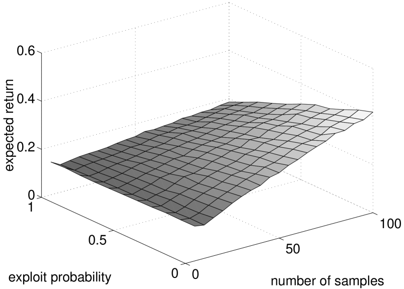
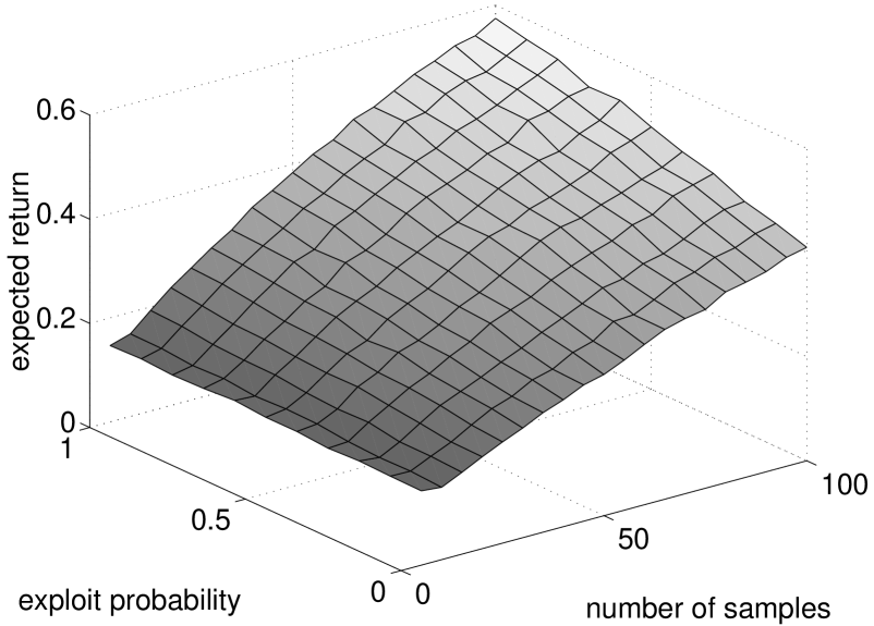
Figure 2: Results for the bandit problems. Top: “HT”: hidden treasure. Bottom: “HF”: hidden failure. Plotted is the expected return of the resulting policy against the number of sample taken, $N$, and the probability of exploiting, $p^{*}$.

Let us consider a trivial example of a bandit problem to illustrate the importance of exploitation and exploration. The environment has a degenerate state space of one state, in which two actions, $a_{1}$ and $a_{2}$, are available. The space of policies available is stochastic and encoded with one parameter, the probability of taking the first action, which is constrained to be in the interval $[\underline{c},\overline{c}]=[.1,.9]$. We consider two problems, called “HT” (hidden treasure) and “HF” (hidden failure) both of which have the same expected returns for actions: $1$ for $a_{1}$ and $0$ for $a_{2}$. In HF, $a_{1}$ always returns $1$, while $a_{2}$ returns $10$ with probability $.99$ and $-990$ with probability $.01$. In HT, $a_{2}$ always returns $0$, while $a_{1}$ returns $-10$ with probability $.99$ and $+1090$ with probability $.01$. We would expect a greedy learning algorithm to sample near policies that look better under scarce information, tending to choose the sub-optimal $a_{2}$ in the HT problem. This strategy is inferior to blind sampling, which samples uniformly from the policy space and will discover the hidden treasure of $a_{1}$ faster. By contrast, for the HF problem we would expect the greedy algorithm to do better by initially concentrating on the $a_{2}$, which looks better, and discovering the hidden failure sooner than blind sampling.

We ran the learn algorithm from table 3 for different settings of the parameters $N$ and $p^{*}$. Figure 2 shows the true value of the resulting policies, averaged over $1000$ runs of the algorithm. While the plots may look discouraging, remember that these problems are in some ways a worse-case situation. The true value of the actions only becomes apparent after sampling on the order of $100$ times. The plots support our hypothesis about the relative success of exploitation. However, although acting greedily is somewhat better in HF, it is much worse in HT. This illustrates why, without any prior knowledge of the domain and given a limited number of samples, it is important not to guide sampling too much by optimization.

5 How Much to Sample?

Table 4: Comparison of sample complexity bounds.

Algorithm	Lower bound on sample complexity $N$
likelihood ratio	$\left(\dfrac{V_{\rm max}}{\epsilon}\right)^{2}2^{4T}(1-\underline{c})^{4T}\left({\cal{K}}(\Theta)+\log(8/\delta)\right)$
reusable trajectories	$\left(\dfrac{V_{\rm max}}{\epsilon}\right)^{2}2^{2T}VC(\Theta)\left(T+\log\left(\dfrac{V_{\rm max}}{\epsilon}\right)+\log(1/\delta)\right)\log(T)$

If we wish to guarantee with probability $1-\delta$ that the error in the estimate of the value function is less than $\epsilon$, we can derive bounds on the necessary sample size $N$, which depend on $\delta$, $\epsilon$, $V_{max}$, and the complexity of the hypothesis class expressed by the covering number ${\cal N}$. Our new result is an extension of the sample complexity bound for the is estimator (Peshkin01) to the wis estimator. We only quote the results here. The key point in the derivation is the fact that

$$\sup_{\bar{h},\bar{h}^{\prime}\in H}\left|\hat{V}^{\rm WIS}_{\bar{h}}-\hat{V}^{\rm WIS}_{\bar{h}^{\prime}}\right|\leq\frac{V_{max}\overline{c}^{T}}{N\underline{c}^{T}+\overline{c}^{T}}\,\,,$$

where $\bar{h}^{\prime}$ differs from $\bar{h}$ only by one member trajectory $h_{i}$. Two inequalities follow from this fact. Denote $\eta=\max(\overline{c}^{T},(1-\underline{c})^{T})$. The variance of the wis estimator according to Devroye’s theorem is bounded as

$${\rm Var}\left\{\hat{V}^{\rm WIS}_{\bar{h}}\right\}\leq\frac{V^{2}_{max}\eta^{4}N}{4(N+\eta^{2})^{2}}$$

and McDiarmid’s theorem ? (?) gives us a pac bound (for derivation see ? (?)):

$$\delta=\Pr\left(\sup_{\theta\in\Theta}\left|\hat{V}^{\rm WIS}(\theta)-{\rm E}\left[\hat{V}^{\rm WIS}(\theta)\right]\right|>\epsilon\right)\\ \leq 4{{\cal N}\left(\Theta,\frac{\epsilon}{8}\right)}\exp\left[-\frac{\epsilon^{2}(N+\eta^{2})^{2}}{32V^{2}_{max}\eta^{4}N}\right]\;,$$

which gives a sample complexity bound very similar to these obtained by ? (?) (see next section). It is well known (Rubinstein81) that variance of wis estimate is $O(\frac{1}{N})$. The weak dependence on the horizon $T$ is interesting and in accordance with empirical findings. The covering number is defined through the value $V(\theta)$ and describes the complexity of a policy class (e.g. reactive policies or finite state controllers) with respect to the structure of a reward function.

5.1 Comparison to vc Bound

The pioneering work by ? (?) considers the issue of generating enough information to determine the near-best policy. We compare our sample complexity results from above with a similar result for their “reusable trajectories” algorithm. Using a random policy (selecting actions uniformly at random), reusable trajectories generates a set of history trees. This information is used to define estimates that uniformly converge to the true values. The algorithm relies on having a generative model of the environment, which allows simulation of a reset of the environment to any state and the execution of any action to sample an immediate reward. The reuse of information is partial: the estimate of a policy value is built only on the subset of experiences that are “consistent” with the estimated policy.

We will make a comparison based on a sampling policy that selects one of two actions uniformly at random: $\Pr(a|h)=\frac{1}{2}$. For the horizon $T$, this gives us an upper bound $\eta$ on the likelihood ratio:

$$w_{\theta}(h,\theta^{\prime})\leq 2^{T}(1-\underline{c})^{T}=\eta\,\,.$$

Substituting this expression for $\eta$, we can compare our bounds to the bound of ? (?) as presented in table 4. The metric entropy ${\cal{K}}(\Theta)$ takes the place of the VC dimension $VC(\Theta)$ in terms of policy class complexity. Metric entropy is a more refined measure of capacity than VC dimension; the VC dimension is an upper bound on the growth function which is an upper bound on the metric entropy (Vapnik98).

5.2 Illustration: Load-Unload Problem

Figure 3: Diagram of the “load-unload” world. The agent observes its position (box) but not whether the cart is loaded (node within the box). The cart loads in the left-most state. If it reaches the right-most position while loaded (upper path), it unloads and gets a unit of reward. The agent has a choice of moving left or right at each position. Each trial begins in the “load” state and lasts $100$ steps. The optimal controller requires one bit of memory.

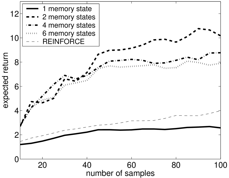
Figure 4: The expected return of the policy found by the algorithm as a function of the number of samples for the environment shown in figure 5.2. The exploitation parameter, $p^{*}$, was set to $0.5$. These results are averaged over $80$ separate runs for each number of samples. The solid line plots the performance using a reactive policy (no memory). The dashed and dotted lines are for policies with differing amounts of memory. Notice that while the reactive policy class converges more quickly, its optimum is much lower. All of the other policy classes have the potential to converge to the optimal return of $13$. However, increased policy complexity results in slower learning.

The complexity of the problem is measured by the covering number, ${\cal N}$. It encodes the complexity of the combination of the pomdp and the policy class. We use the load-unload problem of figure 5.2 to illustrate the effect of policy complexity. The agent is a cart designed to shuttle loads back and forth between two end-points on a line. The cart does not have sensors to indicate whether it is loaded or unloaded, but it can determine its position on the line. The optimal policy is one where the cart moves back and forth between the leftmost and rightmost states moving as many loads as possible. To do so requires some form of memory. For our example, we will use finite-state controllers with fixed memory sizes (SheltonPhD; PeshkinPhD).

A finite-state controller is a class of policies with a fixed memory size. The controller has its own internal memory state that is restricted to one of a finite number of values. At each time step, it not only selects which action to take, but also a memory state for the next time step. The controller’s choice of action and next memory state are independent of the past given the current observation and memory state. This model is an extension of the reactive policy class to allow the controller to remember a small amount about the past. Finite-state controllers have the capability of remembering information for an arbitrarily long period of time.

Figure 4 demonstrates the effect of policy complexity on the performance of the algorithm. This plot is the same as the ones in figure 2 except that the exploitation probability, $p^{*}$, has been fixed at $0.5$. The four lines depict results for different policy classes, $\Theta$. The solid line is for reactive policies (policies with no memory) whereas the dashed and dotted lines are for finite-state controllers with varying amounts of memory. Only one bit of memory is required to perform optimally in this environment. Using more than two states of memory is superfluous. We can see that the simpler the policy class, the more quickly the algorithm converges. However, with too simple a policy class (i.e. reactive policies), the convergence is to a suboptimal policy. For comparison, the thin dashed line presents the behaviour of reinforce with two internal state controller. As we have seen reinforce forgets past experience and picks up very slowly with the size of experience.

6 Discussion

Likelihood-ratio estimation seem to show promise in using data efficiently. The pick_sample routine we present here is only one (simplistic) method of balancing exploitation and exploration. More sophisticated methods including maintaining a distribution over the space of policies might allow for a better balance and the possibility of learning a useful sampling bias in a policy space for a particular application domain and transferring it from one learning problem in that domain to another. In general, estimating the variance of the proxy evaluator could aid in selecting new samples for either exploration or exploitation.

Where reinforce keeps only the most recent sample, our algorithm keeps all of the samples. If a large amount of data is collected, it may be necessary to employ a method between these two extremes and remember a representative set of the samples. Deciding which samples to “forget” would be a difficult, but crucial, task.

Sample complexity bounds depend on the covering number as a measure of the complexity of the policy space. Estimating the covering number is a challenging problem in itself. However it would be more desirable to find a constructive solution to a covering problem in a sense of universal prediction theory  (Merhav98; Shtarkov87). Obviously, given a covering number there might be several ways to cover the space. Finding a covering set would be equivalent to reducing a global optimization problem to an evaluation of several representative policies.

Another way to use sample complexity results is to find what is the minimal experience necessary to be able to provide the estimate for any policy in the class with a given confidence. This would be similar to the structural risk minimization principal by Vapnik ? (?). The intuition is that given very limited data, one might prefer to search a primitive class of hypotheses with high confidence, rather than to get lost in a sophisticated class of hypotheses due to low confidence.

Acknowledgments

The authors would like to thank Leslie Kaelbling for helpful discussions and comments on the manuscript. C.S. was supported by grants from ONR contracts Nos. N00014-93-1-3085 & N00014-95-1-0600, and NSF contracts Nos. IIS-9800032 & DMS-9872936 while at MIT and by ONR contract N00014-00-1-0637 under the MURI program “Decision Making under Uncertainty” while at Stanford. L.P. was supported by ARO grant #DAA19-01-1-0601.

References

- Baird & Moore, (1999) Baird and Moore][1999]Baird99 Baird, L. C., & Moore, A. W. (1999). Gradient descent for general reinforcement learning. Advances in Neural Information Processing Systems (pp. 968–974).
- Baxter & Bartlett, (2000) Baxter and Bartlett][2000]BaxterICML00 Baxter, J., & Bartlett, P. (2000). Reinforcement learning in POMDP’s via direct gradient ascent. Proceedings of the Seventeenth International Conference on Machine Learning (pp. 41–48).
- Glynn, (1986) Glynn][1986]Glynn86 Glynn, P. W. (1986). Optimization of stochastic systems. Proceedings of the Winter Simulation Conference.
- Glynn, (1989) Glynn][1989]Glynn89 Glynn, P. W. (1989). Importance sampling for stochastic simulations. Management Science, 35, 1367–1392.
- Glynn, (1990) Glynn][1990]Glynn90 Glynn, P. W. (1990). Likelihood ratio gradient estimation for stochastic systems. Communications of the ACM, 33, 75–84.
- Glynn, (1994) Glynn][1994]Glynn94 Glynn, P. W. (1994). Importance sampling for Markov chains: asymptotics for the variance. Communication Statistics — Stochastic Models, 10, 701–717.
- (7) Kearns et al.][1999a]KearnsNIPS99 Kearns, M., Mansour, Y., & Ng, A. Y. (1999a). Approximate planning in large POMDPs via reusable trajectories. Advances in Neural Information Processing Systems (pp. 1001–1007).
- (8) Kearns et al.][1999b]KearnsTR99 Kearns, M., Mansour, Y., & Ng, A. Y. (1999b). Approximate planning in large POMDPs via reusable trajectories (Technical Report). AT&T.
- Marbach, (1998) Marbach][1998]Marbach Marbach, P. (1998). Simulation-based methods for Markov decision processes. Doctoral dissertation, MIT.
- McDiarmid, (1989) McDiarmid][1989]McDiarmid89 McDiarmid, C. (1989). Surveys in combinatorics, chapter On the method of bounded differences, 148–188. Cambridge University Press.
- Merhav & Feder, (1998) Merhav and Feder][1998]Merhav98 Merhav, N., & Feder, M. (1998). Universal prediction. IEEE Transactions on Information Theory, 44, 2124–2147. Invited paper.
- Meuleau et al., (2000) Meuleau et al.][2000]MeuleauTR00 Meuleau, N., Peshkin, L., & Kim, K.-E. (2000). Exploration in gradient-based reinforcement learning (Technical Report AIMEMO-1713). MIT.
- Meuleau et al., (1999) Meuleau et al.][1999]MeuleauUAI99 Meuleau, N., Peshkin, L., Kim, K.-E., & Kaelbling, L. P. (1999). Learning finite-state controllers for partially observable environments. Proceedings of the Fifteenth Conference on Uncertainty in Artificial Intelligence (pp. 427–436). Morgan Kaufmann.
- Ormoneit & Glynn, (2000) Ormoneit and Glynn][2000]Glynn00 Ormoneit, D., & Glynn, P. W. (2000). Kernel-based reinforcement learning in average-cost problems: An application to optimal portfolio choice. Advances in Neural Information Processing Systems (pp. 1068–1074).
- Peshkin, (2001) Peshkin][2001]PeshkinPhD Peshkin, L. (2001). Architectures for policy search. Doctoral dissertation, Brown University, Providence, RI 02912.
- Peshkin et al., (2000) Peshkin et al.][2000]Peshkin00 Peshkin, L., Kim, K.-E., Meuleau, N., & Kaelbling, L. P. (2000). Learning to cooperate via policy search. Sixteenth Conference on Uncertainty in Artificial Intelligence (pp. 307–314). San Francisco, CA: Morgan Kaufmann.
- Peshkin et al., (1999) Peshkin et al.][1999]Peshkin99 Peshkin, L., Meuleau, N., & Kaelbling, L. P. (1999). Learning policies with external memory. Proceedings of the Sixteenth International Conference on Machine Learning (pp. 307–314). San Francisco, CA: Morgan Kaufmann.
- Peshkin & Mukherjee, (2001) Peshkin and Mukherjee][2001]Peshkin01 Peshkin, L., & Mukherjee, S. (2001). Bounds on sample size for policy evaluation in Markov environments. Proceedings of the Fourteenth Annual Conference on Computational Learning Theory (pp. 608–615).
- Precup et al., (2000) Precup et al.][2000]PrecupICML00 Precup, D., Sutton, R. S., & Singh, S. P. (2000). Eligibility traces for off-policy policy evaluation. Proceedings of the Seventeenth International Conference on Machine Learning (pp. 759–766).
- Rubinstein, (1981) Rubinstein][1981]Rubinstein81 Rubinstein, R. Y. (1981). Simulation and the Monte Carlo method. New York, NY: Wiley.
- (21) Shelton][2001a]SheltonPhD Shelton, C. R. (2001a). Importance sampling for reinforcement learning with multiple objectives. Doctoral dissertation, MIT.
- (22) Shelton][2001b]Shelton01 Shelton, C. R. (2001b). Policy improvement for POMDPs using normalized importance sampling. Proceedings of the Seventeenth Conference on Uncertainty in Artificial Intelligence (pp. 496–503).
- Shtarkov, (1987) Shtarkov][1987]Shtarkov87 Shtarkov, Y. M. (1987). Universal sequential coding of single measures. Problems of Information Transmission, 175–185.
- Sutton & Barto, (1998) Sutton and Barto][1998]SutBar98 Sutton, R. S., & Barto, A. G. (1998). Reinforcement learning: An introduction. The MIT Press.
- Sutton et al., (1999) Sutton et al.][1999]SuttonNIPS99 Sutton, R. S., McAllester, D., Singh, S. P., & Mansour, Y. (1999). Policy gradient methods for reinforcement learning with function approximation. Advances in Neural Information Processing Systems (pp. 1057–1063).
- Szepesvari, (1999) Szepesvari][1999]Csaba Szepesvari, C. (1999). personal communication.
- Vapnik, (1998) Vapnik][1998]Vapnik98 Vapnik, V. (1998). Statistical learning theory. Wiley.
- Williams & Peng, (1991) Williams and Peng][1991]Williams91 Williams, R., & Peng, J. (1991). Function optimization using connectionist reinforcement learning algorithms. Connection Science, 3, 241–268.
- Williams, (1992) Williams][1992]Williams92 Williams, R. J. (1992). Simple statistical gradient-following algorithms for connectionist reinforcement learning. Machine Learning, 8, 229–256.