The Geometric Maximum Traveling Salesman Problem

Abstract

We consider the traveling salesman problem when the cities are points in ${\mathbb{R}^{d}}$ for some fixed $d$ and distances are computed according to geometric distances, determined by some norm. We show that for any polyhedral norm, the problem of finding a tour of maximum length can be solved in polynomial time. If arithmetic operations are assumed to take unit time, our algorithms run in time $O(n^{f-2}\log n)$, where $f$ is the number of facets of the polyhedron determining the polyhedral norm. Thus for example we have $O(n^{2}\log n)$ algorithms for the cases of points in the plane under the Rectilinear and Sup norms. This is in contrast to the fact that finding a minimum length tour in each case is NP-hard. Our approach can be extended to the more general case of quasi-norms with not necessarily symmetric unit ball, where we get a complexity of $O(n^{2f-2}\log n)$.

For the special case of two-dimensional metrics with $f=4$ (which includes the Rectilinear and Sup norms), we present a simple algorithm with $O(n)$ running time. The algorithm does not use any indirect addressing, so its running time remains valid even in comparison based models in which sorting requires $\Omega(n\log n)$ time. The basic mechanism of the algorithm provides some intuition on why polyhedral norms allow fast algorithms.

Complementing the results on simplicity for polyhedral norms, we prove that for the case of Euclidean distances in ${\mathbb{R}^{d}}$ for $d\geq 3$, the Maximum TSP is NP-hard. This sheds new light on the well-studied difficulties of Euclidean distances.

1 Introduction

In the Traveling Salesman Problem (TSP), the input consists of a set $C$ of cities together with the distances $d(c,c^{\prime})$ between every pair of distinct cities $c,c^{\prime}\in C$. The goal is to find an ordering or tour of the cities that minimizes (Minimum TSP) or maximizes (Maximum TSP) the total tour length. Here the length of a tour $c_{\pi(1)},c_{\pi(2)},\ldots,c_{\pi(n)}$ is

$$\sum_{i=1}^{n-1}d(c_{\pi(i)},c_{\pi(i+1)})+d(c_{\pi(n)},c_{\pi(1)}).$$

Like the Minimum TSP, the Maximum TSP is NP-complete on graphs, even if the triangle inequality holds. After 25 years, the best known performance guarantee for the metric Minimum TSP is still Christofides’s 3/2 approximation algorithm; the results of Arora, Lund, Motwani, Sudan, and Szegedy [4] show that the problem cannot be approximated arbitrarily well, combined with results by Papadimitriou and Yannakakis [26], it follows that this holds even for the special class of instances where all distances are 1 or 2. There has been more development on approximation algorithms for the metric Maximum TSP: Recently, Hassin and Rubinstein [18] have given a 7/8 approximation algorithm.

Of particular interest are geometric instances of the TSP, in which cities correspond to points in ${\mathbb{R}^{d}}$ for some $d\geq 1$, and distances are computed according to some geometric norm. Perhaps the most popular norms are the Rectilinear, Euclidean, and Sup norms. These are examples of what is known as an “$L_{p}$ norm” for $p=1$, $2$, and $\infty$. In general, the distance between two points ${\bit x}=(x_{1},x_{2},\ldots,x_{d})$ and ${\bit y}=(y_{1},y_{2},\ldots,y_{d})$ under the $L_{p}$ norm, $p\geq 1$, is

$$d({\bit x},{\bit y})=\left(\sum_{i=1}^{d}\left|x_{i}-y_{i}\right|^{p}\right)^{1/p}$$

with the natural asymptotic interpretation that distance under the $L_{\infty}$ norm is

$$d({\bit x},{\bit y})=\max{}_{i=1}^{d}\left|x_{i}-y_{i}\right|.$$

This paper considers a second class of norms which also includes the Rectilinear and Sup norms, but can only approximate the Euclidean and other $L_{p}$ norms. This is the class of polyhedral norms. Each polyhedral norm is determined by a unit ball which is a centrally-symmetric polyhedron ${\bit P}$ with the origin at its center. To determine $d({\bit x},{\bit y})$ under such a norm, first translate the space so that one of the points, say ${\bit x}$, is at the origin. Then determine the unique factor $\alpha$ by which one must rescale ${\bit P}$ (expanding if $\alpha>1$, shrinking if $\alpha<1$) so that the other point (${\bit y}$) is on the boundary of the polyhedron. We then have $d({\bit x},{\bit y})=\alpha$.

Alternatively, and more usefully for our purposes, we can view a polyhedral norm as follows. If ${\bit P}$ is a polyhedron as described above and has $f$ facets, then $f$ is divisible by 2 and there is a set $H_{\bit P}=\{{\bit h}_{1},\ldots,{\bit h}_{f/2}\}$ of points in ${\mathbb{R}^{d}}$ such that ${\bit P}$ is the intersection of a collection of half-spaces determined by $H_{{\bit P}}$:

$${\bit P}=\left(\bigcap_{i=1}^{f/2}\{{\bit x}:~{}{\bit x}\cdot{\bit h}_{i}\leq 1\}\right)\cap\left(\bigcap_{i=1}^{f/2}\{{\bit x}:~{}{\bit x}\cdot{\bit h}_{i}\geq-1\}\right).$$

Then we have

$$d({\bit x},{\bit y})=\max\Big{\{}\Big{|}({\bit x}-{\bit y})\cdot{\bit h}_{i}\Big{|}:~{}1\leq i\leq{f/2}\Big{\}}.$$

Note that for the Rectilinear norm in the plane we can take $H_{{\bit P}}$ = $\{(1,1),(-1,1)\}$ and for the Sup norm in the plane we can take $H_{{\bit P}}$ = $\{(1,0),(0,1)\}$.

For the Minimum TSP on geometric instances, two key complexity questions have been answered. As follows from results of Itai, Papadimitriou, and Swarcfiter [19], the Minimum TSP is NP-hard for any fixed dimension $d$ and any $L_{p}$ or polyhedral norm; see also the earlier results by Garey, Graham, and Johnson [15], and Papadimitriou [25]. On the other hand, results of Arora [3] and Mitchell [23] imply that in all these cases a polynomial-time approximation scheme (PTAS) exists, i.e., a sequence of polynomial-time algorithms $A_{k}$, $1\leq k<\infty$, where $A_{k}$ is guaranteed to find a tour whose length is within a ratio of $1+(1/k)$ of optimal.

The situation for geometric versions of the Maximum TSP has been less clear than for its minimum counterpart. Serdyukov [28], and, independently, Barvinok [6], have shown that once again polynomial-time approximation schemes exist for all fixed dimensions $d$ and all $L_{p}$ or polyhedral norms (and in a sense for any fixed norm; see [6]). Until now, however, the complexity of the optimization problems themselves when $d$ is fixed has remained open: For no fixed dimension $d$ and $L_{p}$ or polyhedral norm was the problem of determining the maximum tour length known either to be NP-hard or to be polynomial-time solvable. In this paper, we resolve the question for all polyhedral norms, showing that, in contrast to the case for the Minimum TSP, the Maximum TSP is solvable in polynomial time for any fixed dimension $d$ and any polyhedral norm:

Theorem 1

Let dimension $d$ be fixed, and let $\parallel\cdot\parallel$ be a fixed polyhedral norm in ${\mathbb{R}^{d}}$ whose unit ball is a centrally symmetric polyhedron ${\bit P}$ determined by a set of $f$ facets. Then for any set of $n$ points in ${\mathbb{R}^{d}}$, one can construct a traveling salesman tour of maximum length with respect to $\parallel\cdot\parallel$ in time $O(n^{f-2}\log n)$ in the real number RAM model, where arithmetic operations take unit time and only addition, subtraction, multiplication, and division are allowed.

A similar result also holds for polyhedral quasi-norms, i.e., asymmetric distance functions that can be defined in terms of “unit balls” that are non-symmetric polyhedra containing the origin. These can again be characterized by a set of vectors $H_{P}$, but now we need a vector for each facet of the polyhedron and $d(x,y)=\max\left\{(x-y)\cdot h~{}:~{}h\in H_{P}\right\}$. Serdyukov [28, 29] previously showed that for the case of a quasi-norm in ${\mathbb{R}^{2}}$ with a triangle as the unit ball, the Maximum TSP can be solved in polynomial time. With our techniques we can show the following analog of Theorem 1.

Theorem 2

Let dimension $d$ be fixed, and let $\parallel\cdot\parallel$ be a fixed polyhedral quasi-norm in ${\mathbb{R}^{d}}$ whose unit ball is a polyhedron ${\bit P}$ determined by a set of $f$ facets. Then for any set of $n$ points in ${\mathbb{R}^{d}}$, one can construct a traveling salesman tour of maximum length with respect to $\parallel\cdot\parallel$ in time $O(n^{2f-2}\log n)$ in the real number RAM model.

As an immediate consequence of Theorem 1, we get relatively efficient algorithms for the Maximum TSP in the plane under Rectilinear and Sup norms, with a complexity of $O(n^{2}\log n)$.

The restriction to the real number RAM model in Theorem 1 is made primarily to simplify the statements of the conclusions. Suppose on the other hand that one assumes, as one typically must for complexity theory results, that the components of the vectors in $H_{\bit P}$ and the coordinates of the cities are all rationals. Let $U$ denote the maximum absolute value of any of the corresponding numerators and denominators. Then the conclusions of the Theorem hold for the standard logarithmic cost RAM model with running times multiplied by $n\log(U)$. If the components/coordinates are all integers with maximum absolute value $U$, the running times need only be multiplied by $\log(nU)$. For simplicity in the remainder of this paper, we shall stick to the model in which numbers can be arbitrary reals and arithmetic operations take unit time. The reader should have no trouble deriving the above variants.

The above results make use of a polynomial solution method for the following TSP variant, which may be of independent interest: When visiting a given set of $n$ cities, all connections have to be made via a set of $k$ hubs, where $k$ is a constant.

The complexity of $O(n^{2}\log n)$ for the scenario of planar rectilinear distances can be improved by using special geometric properties of this case. We can show the following optimal running time:

Theorem 3

The Maximum TSP for points in ${\mathbb{R}^{2}}$ under the $L_{1}$ norm can be solved in $O(n)$ time.

By appropriate coordinate transformation, this result can be generalized to all planar polyhedral norms with $f=4$ facets, which includes the Sup norm. It holds even in a restricted model of computation, where no indirect addressing may be used, and hence sorting requires $\Omega(n\log n)$ time. The main idea behind the algorithm is to exploit the fact that rectilinear distances in the plane have a high degree of degeneracy. As a consequence, we can show that the number of optimal tours is very large, $\Omega\left((\frac{n}{4}!)^{4}\right)$, and the set of optimal tours can be described very easily. This contrasts sharply to the case of Euclidean distances, where there may be a single optimal tour.

Indeed the complexity of the Maximum TSP in ${\mathbb{R}^{2}}$ under the Euclidean metric remains an open question, although we have resolved the question for higher dimensions with the following result.

Theorem 4

Maximum TSP under Euclidean distances in ${\mathbb{R}^{d}}$ is an NP-hard problem if $d\geq 3$.

One of the consequences is NP-hardness of the Maximum TSP for polyhedral norms with an unbounded number of facets on the corresponding unit ball. Another consequence concerns the so-called Maximum Scatter TSP, where the objective is to find a tour that maximizes the shortest edge. The Maximum Scatter TSP was first considered by Arkin, Chiang, Mitchell, Skiena, and Yang [2], and the complexity for geometric instances was stated as an open problem. Our result implies NP-hardness for Euclidean instances in 3-dimensional space.

An issue that is still unresolved for the Maximum TSP as well as the Minimum TSP is the question of whether the TSP under Euclidean distances is a member of the class NP, allowing polynomial time verification of a good solution. Even if all city coordinates are rationals, we do not know how to compare a tour length to a given rational target in less than exponential time. Such a comparison would appear to require us to evaluate a sum of $n$ square roots to some precision, and currently the best upper bound known on the number of bits of precision needed to insure a correct answer remains exponential in $n$.

The rest of this paper is organized as follows. Section 2 introduces a new special case of the TSP, the Tunneling TSP. We show how the Maximum TSP under a polyhedral norm can be reduced to the Tunneling TSP with the same number of cities and $k=f/2$ tunnels (and with $k=f$ tunnels for polyhedral quasi-norms). Section 3.1 shows how the solutions for the Tunneling TSP with a fixed number $k\geq 2$ of tunnels can be characterized, setting up an algorithm with a running time of $O(n^{2k-2}\log n)$ described in detail in Section 3.2. Section 4 describes the linear-time algorithm for rectilinear distances in the plane. Section 5 gives the NP-hardness proof of the Maximum Traveling Salesman Problem for Euclidean distances in ${\mathbb{R}^{3}}$, and a number of higher-dimensional extensions. Section 6 concludes with a brief discussion and open problems.

2 The Tunneling TSP

The Tunneling TSP is a special case of the Maximum TSP in which distances are determined by what we shall call a tunnel system distance function. In such a distance function we are given a set $T=\{t_{1},t_{2},\ldots,t_{k}\}$ of $k\geq 2$ auxiliary objects that we shall call tunnels. Each tunnel is viewed as a bidirectional passage having a front and a back end. For each pair $c,t$ of a city and a tunnel we are given real-valued access distances $F(c,t)$ and $B(c,t)$ from the city to the front and back ends of the tunnel respectively. Each potential tour edge $\{c,c^{\prime}\}$ must pass through some tunnel $t$, either by entering the front end and leaving the back (for a distance of $F(c,t)+B(c^{\prime},t)$), or by entering the back end and leaving the front (for a distance of $B(c,t)+F(c^{\prime},t)$). Since we are looking for a tour of maximum length, we can thus define the distance between cities $c$ and $c^{\prime}$ to be

$$d(c,c^{\prime})=\max\Big{\{}F(c,t_{i})+B(c^{\prime},t_{i}),\;B(c,t_{i})+F(c^{\prime},t_{i}):1\leq i\leq k\Big{\}}$$

Note that this distance function, like our geometric norms, is symmetric. (As we will see below, we can make adjustments for asymmetric distance functions.)

It is easy to see that Maximum TSP remains NP-hard when distances are determined by arbitrary tunnel system distance functions. However, for the case where $k=|T|$ is fixed and not part of the input, we will show in the next section that Maximum TSP can be solved in $O(n^{2k-2}\log n)$ time. We are interested in this special case because of the following lemma.

Lemma 5

If $\parallel\cdot\parallel$ is a polyhedral norm determined by a set $H_{\bit P}$ of $k=f/2$ vectors in ${\mathbb{R}^{d}}$, then for any set $C$ of points in ${\mathbb{R}^{d}}$ one can in time $O(dk|C|)$ construct a tunnel system distance function with $k$ tunnels that yields $d({\bit c},{\bit c^{\prime}})=\parallel{\bit c}-{\bit c^{\prime}}\parallel$ for all ${\bit c},{\bit c^{\prime}}\in C$.

Proof: The polyhedral distance between two cities $\parallel{\bit c},{\bit c^{\prime}}\parallel\in{\mathbb{R}^{d}}$ is

$$\parallel{\bit c}-{\bit c^{\prime}}\parallel = \max\Big{\{}\Big{|}({\bit c}-{\bit c^{\prime}})\cdot{\bit h}_{i}\Big{|}:~{}1\leq i\leq k\Big{\}}$$

$$= \max\Big{\{}({\bit c}-{\bit c^{\prime}})\cdot{\bit h}_{i},\;({\bit c^{\prime}}-{\bit c})\cdot{\bit h}_{i}:~{}1\leq i\leq k\Big{\}}$$

Thus we can view the distance function determined by $\parallel\cdot\parallel$ as a tunnel system distance function with set of tunnels $T=H_{\bit P}$ and $F({\bit c},{\bit h})={\bit c}\cdot{\bit h}$, $B({\bit c},{\bit h})=-{\bit c}\cdot{\bit h}$ for all cities ${\bit c}$ and tunnels ${\bit h}$. $\Box$

It is straightforward to extend this characterization to the case of any polyhedral quasi-norm that is characterized by a unit ball with a total of $f$ facets. The only real change is in the complexity of the characterization of the tunnel system in Lemma 5. If we use the definition

$$\tilde{d}(c,c^{\prime})=\max\Big{\{}F(c,t_{i})+B(c^{\prime},t_{i}):1\leq i\leq k\Big{\}}$$

for possibly asymmetric tunnel distances, then by similar reasoning we get the following:

Lemma 6

If $\parallel\cdot\parallel$ is a polyhedral quasi-norm determined by a set $H_{\bit P}$ of $f$ vectors in ${\mathbb{R}^{d}}$, then for any set $C$ of points in ${\mathbb{R}^{d}}$ one can in time $O(df|C|)$ construct a tunnel system distance function with $f$ tunnels that yields $\tilde{d}({\bit c},{\bit c^{\prime}})=\parallel{\bit c}-{\bit c^{\prime}}\parallel$ for all ${\bit c},{\bit c^{\prime}}\in C$.

3 An Algorithm for Bounded Tunnel Systems

In this section we describe an $O(n^{2k-2}\log n)$ algorithm to solve the Tunneling TSP when the number of tunnels is fixed at $k$, assuming the real number RAM model. By Lemmas 5 and 6 this implies our results for polyhedral norms and quasi-norms (Theorems 1 and 2.) The approach described below also yields a polynomial algorithm for a Minimum TSP variant, where a given set of $n$ cities has to be traveled, and all connections have to be made via a set of a fixed number $k$ of hubs.

We start by characterizing solutions for bounded tunnel systems in Section 3.1. This characterization is the basis for our algorithm, which is described in Section 3.2. In Section 3.3 we present an additional idea that may possibly improve the above complexity to $O(n^{2k-2})$.

3.1 Characterizing Solutions for Bounded Tunnel Systems

We start by discussing the solutions for bounded tunnel systems.

Suppose we are given an instance of the Tunneling TSP with sets $C=\{c_{1},\ldots,c_{n}\}$ and $T=\{t_{1},\ldots,t_{k}\}$ of cities and tunnels, and access distances $F(c,t)$, $B(c,t)$ for all $c\in C$ and $t\in T$. We begin by transforming the problem to one about subset construction.

Let $G=(C\cup T,E)$ be an edge-weighted, bipartite multigraph with four edges between each city $c$ and tunnel $t$, denoted by $e_{i}[c,t,X]$, $i\in\{1,2\}$ and $X\in\{B,F\}$. The weights of these edges are $w(e_{i}[c,t,F])=F(c,t)$ and $w(e_{i}[c,t,B])=B(c,t)$, $i\in\{1,2\}$. For notational convenience, let us partition the edges in $E$ into sets $E[t,F]=\{e_{i}[c,t,F]:c\in C,i\in\{1,2\}\}$ and $E[t,B]=\{e_{i}[c,t,B]:c\in C,i\in\{1,2\}\}$, $t\in T$. Each tour for the TSP instance then corresponds to a subset $E^{\prime}$ of $E$ that has $\sum_{e\in E^{\prime}}w(e)$ equal to the tour length and satisfies

• Every city is incident to exactly two edges in $E^{\prime}$.

• For each tunnel $t\in T$, $|E^{\prime}\cap E[t,F]|=|E^{\prime}\cap E[t,B]|$.

• The set $E^{\prime}$ is connected.

To construct the multiset $E^{\prime}$, we simply represent each tour edge $\{c,c^{\prime}\}$ by a pair of edges from $E$ that connect in the appropriate way to the tunnel that determines $d(c,c^{\prime})$. For example, if $d(c,c^{\prime})=F(c,t)+B(c^{\prime},t)$, and $c$ appears immediately before $c^{\prime}$ when the tour is traversed starting from $c_{\pi(1)}$, then the edge $(c,c^{\prime})$ can be represented by the two edges $e_{2}[c,t,F]$ and $e_{1}[c^{\prime},t,B]$. Note that there are enough (city,tunnel) edges of each type so that all tour edges can be represented, even if a given city uses the same tunnel endpoint for both its tour edges. Also note that if $d(c,c^{\prime})$ can be realized in more than one way, the multiset $E^{\prime}$ will not be unique. However, any multiset $E^{\prime}$ constructed in this fashion will still have $\sum_{e\in E^{\prime}}w(e)$ equal to the tour length.

On the other hand, any set $E^{\prime}$ satisfying (T1) – (T3) corresponds to one (or more) tours having length at least $\sum_{e\in E^{\prime}}w(e)$: Let $T^{\prime}\subseteq T$ be the set of tunnels $t$ with $|E^{\prime}\cap E[t,F]|>0$. Then $G^{\prime}=(C\cup T^{\prime},E^{\prime})$ is a connected graph all of whose vertex degrees are even by (T1) – (T3). By an easy result from graph theory, this means that $G^{\prime}$ contains an Euler tour that by (T1) passes through each city exactly once, thus inducing a TSP tour for $C$. Moreover, by (T2) one can construct such an Euler tour with the additional property that if $e_{i}[c,t,x]$ and $e_{j}[c^{\prime},t,y]$ are consecutive edges in this tour, then $x\neq y$, i.e, either $x=F,y=B$ or $x=B,y=F$. Thus we will have $w(e_{i}[c,t,x])+w(e_{j}[c^{\prime},t,y])\leq d(c,c^{\prime})$, and hence the length of the TSP tour will be at least $\sum_{e\in E^{\prime}}w(e)$, as claimed.

In summary, our problem is reduced to finding a maximum weight set of edges $E^{\prime}\subseteq E$ satisfying (T1) – (T3).

3.2 An Efficient Algorithm

3.2.1 Identifiers for Subproblems

From the previous section we know that our problem is reduced to finding a maximum weight set of edges $E^{\prime}\subseteq E$ satisfying (T1) – (T3). Given that $k$ is fixed, we will first show how to decompose the problem into $O(n^{2k-3})$ instances, and then demonstrate how to solve each one of them in $O(n\log n)$ time.

Let $E^{\prime}$ be a subset of edges satisfying (T1) – (T3). We associate five identifiers with $E^{\prime}$.

The first is $T^{\prime}\subseteq T$, the subset of $p$, $p\leq k$, tunnels that are spanned by $E^{\prime}$. (Without loss of generality suppose that $T^{\prime}=\{t_{1},...,t_{p}\}$.) Globally, the total number of identifiers of the first type is $O(2^{k})$.

Due to conditions (T1), (T3) we know that there is a subset of $2(p-1)$ edges $E^{\prime\prime}\subset E^{\prime}$ such that the subgraph $G(E^{\prime\prime})$, induced by $E^{\prime\prime}$, is connected and it spans $T^{\prime}$ and exactly $p-1$ cities. Moreover, each of these cities is incident to exactly two edges in $E^{\prime\prime}$, which connects two adjacent tunnels in $T^{\prime}$. We use the second, the third and the fourth identifiers to characterize $G(E^{\prime\prime})$.

The second identifier is the spanning tree topology connecting the tunnels of $T^{\prime}$ that is induced by the set of edges $E^{\prime\prime}$. There are $p^{p-2}$ identifiers of this type: the number of labeled spanning trees of $K_{p}$, the complete graph on $p$ nodes [9].

The third identifier is an assignment of distinct cities to the spanning tree edges of the previous identifier. The city assigned to the tree edge joining tunnels $t$ and $t^{\prime}$ is one that is connected by one edge of $E^{\prime\prime}$ to $t$ and by another edge of $E^{\prime\prime}$ to $t^{\prime}$. The total number of identifiers of the third type is $O(n^{p-1})$.

The fourth identifier is the subset of $2(p-1)$ edges linking these cities with corresponding tunnel entrances. In the underlying graph $G$ there are four edges (two pairs of identical edges) connecting a city with a tunnel. Therefore, the total number of identifiers of the fourth type is $O(16^{p-1})$.

The fifth and last identifier is the degree sequence of the nodes in $T^{\prime}$ induced by $E^{\prime}$. Let $d=(2d_{1},...,2d_{p})$ denote this sequence of even positive degrees. Note that $d_{1}+...+d_{p}=n$. Therefore, there are clearly $O(n^{p-1})$ identifiers of this third type. However, we will modify the identifier and use one of the degree entries, say $d_{p}$, as an unspecified parameter. Thus, there are only $O(n^{p-2})$ choices for, say, $d_{1},d_{2},...,d_{p-2}$. ($d_{p-1}$ will then depend linearly on the parameter $d_{p}$.) Altogether, we now have $O(n^{2k-3})$ choices for values of identifiers.

In summary, to prove our claim that the Tunneling TSP can be solved in $O(n^{2k-2}\log n)$ time when $k$ is fixed, it will suffice to show that the following problem can be solved in $O(n\log n)$ time.

Given a set of tunnels $T^{\prime}=\{t_{1},...,t_{p}\}$, a set of $p-1$ cities, a set $E^{\prime\prime}$ of $2(p-1)$ edges connecting the cities to the tunnels as above, and a set of positive integers $d_{1},...,d_{p-2}$, find a maximum weight set of edges $E^{\prime}$, containing $E^{\prime\prime}$, satisfying (T1)-(T2), and such that the degree of $t_{i}$ is $2d_{i}$, $1\leq i\leq p-2$.

3.2.2 Solving the Subproblems

Without loss of generality assume that the $p-1$ cities connecting the tunnels in $T^{\prime}$ are $\{c_{1},...,c_{p-1}\}$. Let $C^{\prime}=\{c_{1},...,c_{p-1}\}$, and $C^{\prime\prime}=C-C^{\prime}$. For each $i=1,...,p$, we split the tunnel $t_{i}$ into two nodes, $t_{i}^{B}$ and $t_{i}^{F}$. They are called, respectively, $B$ and $F$ tunnel entrances. Define $T^{\prime}_{B}=\{t_{1}^{B},...,t_{p}^{B}\}$ and $T^{\prime}_{F}=\{t_{1}^{F},...,t_{p}^{F}\}$.

Let $G^{\prime}=(C^{\prime\prime}\cup(T_{B}^{\prime}\cup T_{F}^{\prime}),E^{*})$ be an edge-weighted, bipartite multigraph with two edges, each of weight $B(c_{j},t_{i})$, connecting $c_{j}$ and $t_{i}^{B}$, $j=p,p+1,...,n$, $i=1,...,p$, and two edges, each of weight $F(c_{j},t_{i})$, connecting $c_{j}$ and $t_{i}^{F}$, $j=p,p+1,...,n$, $i=1,...,p$.

Next, using the notation from the previous subsection, for each $i=1,...,p$, let $f_{i}^{B}=|E^{\prime\prime}\cap E[t_{i},B]|$ and $f_{i}^{F}=|E^{\prime\prime}\cap E[t_{i},F]|$. (Note that $f_{i}^{B}$ ($f_{i}^{F}$) is the number of “back” (“front”) type edges in $E^{\prime\prime}$ that are incident to tunnel $t_{i}$.)

Following is a formal description of the maximization problem:

$$g(d_{p})=\max(\sum_{i=1}^{p}\sum_{j=p}^{n}B(c_{j},t_{i})x_{i,j}^{B}+\sum_{i=1}^{p}\sum_{j=p}^{n}F(c_{j},t_{i})x_{i,j}^{F})$$

subject to

$$\sum_{j=p}^{n}x_{i,j}^{B}=d_{i}-f_{i}^{B},\ i=1,...,p-2,p$$

$$\sum_{j=p}^{n}x_{i,j}^{F}=d_{i}-f_{i}^{F},\ i=1,...,p-2,p$$

$$\sum_{j=p}^{n}x_{p-1,j}^{B}=n-d_{p}-f_{p-1}^{B}-\sum_{i=1}^{p-2}d_{i},$$

$$\sum_{j=p}^{n}x_{p-1,j}^{F}=n-d_{p}-f_{p-1}^{F}-\sum_{i=1}^{p-2}d_{i},$$

$$\sum_{i=1}^{p}(x_{i,j}^{B}+x_{i,j}^{F})=2,\ j=p,...,n,$$

$$x_{i,j}^{B}\geq 0,\ i=1,...,p,\ j=p,...,n,$$

$$x_{i,j}^{F}\geq 0,\ i=1,...,p,\ j=p,...,n.$$

It is easy to see that for each integer value $d_{p}\in\{1,2,...,n\}$, the above problem is an instance of the classical transportation problem with $n-p+1$ sources (cities) and $2p$ destinations ( $p$ B tunnels and $p$ F tunnels). Therefore there is an optimal solution to the linear program for each integer value of $d_{p}$ in which all variables are integer. Moreover, since the number of destinations is fixed ($p\leq k$), when $d_{p}$ is specified the dual of this transportation problem can be solved in $O(n)$ time by the algorithm in Zemel [33]. (See also Megiddo and Tamir [22].) In particular, $g(d_{p})$ can be computed by solving the dual in $O(n)$ time. Viewing $d_{p}$ as a (real) parameter, we note that $g(d_{p})$, the optimal objective value of the above transportation problem, is a concave function of $d_{p}$. To see this, observe that if $d<d^{\prime}$ are legal values for $d_{p}$, and $\bar{x}_{d}$ and $\bar{x}_{d^{\prime}}$ are the optimal solutions for these two values viewed as vectors of variable values, then $(\bar{x}_{d}+\bar{x}_{d^{\prime}})/2$ is a feasible solution for $(d+d^{\prime})/2$ and so $g((d+d^{\prime})/2)\geq(g(d)+g(d^{\prime}))/2$. Thus, we can apply a Fibonacci search over the integers $\{1,2,...,n\}$, or alternatively perform a binary search, at each step checking the values at $d-1$, $d$, and $d+1$. (Actually, $d_{p}$ is restricted by $1\leq d_{p}<n-\sum_{i=1}^{p-2}d_{i}$.) Specifically, by computing the function $g(d_{p})$ at $O(\log n)$ values of $d_{p}$ we obtain the (integer) value of $d_{p}$ maximizing $g(d_{p})$. Thus, in $O(n\log n)$ time we find the best value of $d_{p}$.

Therefore, in time $O(n^{2k-3}\cdot n\log n)=O(n^{2k-2}\log n)$ we can determine the set of identifiers for the transportation problem that yields the maximum solution value (including the full degree sequence for the tunnels). This solution value will be the length of the maximum length tour, but because we were solving the dual rather than primal LP’s, we won’t yet have the optimal tour itself. For this, we need only solve the optimal transportation problem directly in its primal form. Since the number of tunnels is bounded, we can do this in deterministic time $O(n)$ using an algorithm described in an unpublished paper by Matsui [21]. The basic idea is to apply complementary slackness properties to the already computed dual solution variables to reduce the problem to a network flow problem for a bounded number of sinks. This can then be solved in linear time using an algorithm of of Gusfield, Martel and Fernandez-Baca [17] (see also Ahuja, Orlin, Stein and Tarjan [1]). Alternatively, one can use the published algorithm of Tokuyama and Nakano [31] that requires time $O(n\log^{2}n)$ time. In either case, the time to find this one primal solution is dominated by the time already spent to solve all the duals, so the overall running time bound is that for the latter: $O(n^{2k-2}\log n)$.

3.3 Further Improvement

One way to improve upon the above bound is to reduce the running time to solve an instance of the parametric transportation problem from $O(n\log n)$ to $O(n)$. At this point we do not know how to achieve the linear bound, but we feel that the following approach might be fruitful.

Consider the above parametric transportation problem, and view the parameter $d_{p}$ as an additional (real) variable. The resulting linear program, which we call the primal, is not a transportation problem. Nevertheless, the algorithms in Zemel [33] and Megiddo and Tamir [22] can still solve the dual of this linear program in $O(n)$ time. The missing ingredient at this point is how to use the dual solution to obtain (in linear time), an optimal solution to the primal program. Specifically, we only need to know the optimal (real) value of the primal variable $d_{p}$, say $d_{p}^{*}$. If $d_{p}^{*}$ is known, we can use the concavity property of the function $g(d_{p})$ to conclude that the optimal integer value of $d_{p}$ is attained by rounding $d_{p}^{*}$ up or down. We can then proceed as above.

4 An $O(n)$ Algorithm

In this section, we describe a linear-time algorithm for determining the length of an optimal tour for the Maximum TSP under rectilinear distances in the plane. This amounts to a proof of Theorem 3, structured into a series of Lemmas and stretching over Subsections 4.1 to  4.3. At the end of the section we sketch how this result can be extended to any 4-facet polyhedral metric. Throughout this section we assume without loss of generality that $n\geq 4$, as otherwise the problem is trivial.

4.1 Stars and Matchings

Our construction uses properties of so-called stars; a star for a given set of vertices $V$ is a minimum Steiner tree with precisely one Steiner point (the center) that contains all vertices in $V$ as leafs. The total length of the edges in a star is an upper bound on any matching in $V$, since any edge $(v_{i},v_{j})$ in the matching can be mapped to a pair of edges $(v_{i},c)$ and $(c,v_{j})$ in the star, and by triangle inequality, $d(v_{i},v_{j})\leq d((v_{i},c)+d(c,v_{j})$. The worst case ratio between the total length of a minimum star $\min S(P)$ and a maximum matching $\max M(P)$ plays a crucial role in several different types of optimization problems. See the paper by Fingerhut, Suri, and Turner [14] for applications in the context of broadband communication networks. Also, Tamir and Mitchell [30] have used the duality between minimum stars and maximum matchings for showing that certain matching games have a nonempty core. The value of the worst case ratio under the Euclidean metric has been determined by Fekete and Meijer; see [13] for this result and several extensions.

In the rest of this section, all distances are planar rectilinear distances, unless noted otherwise at the end of the section. For rectilinear distances, determining the length $\min S(P)$ of a minimum length star (also known as the rectilinear planar unweighted 1-median or rectilinear Fermat–Weber problem) can be done in linear time.

Lemma 7

Suppose we are given a given set of $n$ points $P=\{p_{1},\ldots,p_{n}\}$ with $p_{i}=(x_{i},y_{i})$, $1\leq i\leq n$. Then under $L_{1}$ distances there is an optimal star center $c=(x_{c},y_{c})$, where $x_{c}$ is a median of $\{x_{i}\mid i=1,\ldots,n\}$, and $y_{c}$ is a median of $\{y_{i}\mid i=1,\ldots,n\}$.

This is problem 9-2e in [10]. Recall that if $n=2m$ is even, then both the $m$’th and $(m+1)$’st largest items are medians.) The proof is immediate; for an $O(n)$ running time, use the result by Blum, Floyd, Pratt, Rivest, and Tarjan [11] for computing a median of $n$ numbers.

It should be noted that for Euclidean distances, the problem of determining $\min S(P)$ is considerably harder: It was shown by Bajaj [5] that the problem of finding an optimal star center for five points in the plane is in general not solvable by radicals over the field of rationals. This implies that an algorithm for computing $\min S(P)$ must use stronger tools than constructions by straight edge and compass.

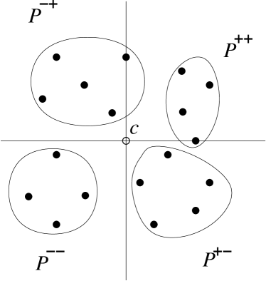
Figure 1: The four quadrants and their point sets.

The following Theorem 8 appears in the paper by Tamir and Mitchell [30] as Theorem 8; independently, it was noted by Fekete and Meijer[13].

Theorem 8

For $|P|$ even, we have $\max M(P)=\min S(P)$ for rectilinear distances in the plane.

The basic idea is that the coordinates of an optimal star center subdivide the plane into four quadrants. If ties are broken in the right way, the number of points in opposite quadrants is the same. See Figure 1. Then

$$L_{1}(v_{i},v_{j})=L_{1}(v_{i},c)+L_{1}(c,v_{j})$$ (1)

holds for any edge $(v_{i},v_{j})$ in the matching, and the theorem follows easily. $\Box$

Since the results of this paper include the case in which $|P|$ is odd, we formalize and generalize this observation.

Let $x_{c}$ and $y_{c}$ be as in Lemma 7 and define $P_{x}^{-}:=\{p_{i}\in P\mid x_{i}<x_{c}\}$, $P_{x}^{0}:=\{x_{i}\mid x_{i}=x_{c}\}$, $P_{x}^{+}:=\{p_{i}\in P\mid x_{i}>x_{c}\}$, $P_{y}^{-}:=\{p_{i}\in P\mid y_{i}<y_{c}\}$, $P_{y}^{0}:=\{y_{i}\mid y_{i}=y_{c}\}$, and $P_{y}^{+}:=\{p_{i}\in P\mid y_{i}>y_{c}\}$, From the above conditions, it follows that

$$n_{x}^{-}: = |P_{x}^{-}|\leq\frac{n}{2}$$ (2)

$$n_{x}^{+}: = |P_{x}^{+}|\leq\frac{n}{2}$$ (3)

$$n_{y}^{-}: = |P_{y}^{-}|\leq\frac{n}{2}$$ (4)

$$n_{y}^{+}: = |P_{y}^{+}|\leq\frac{n}{2}.$$ (5)

Let $n_{x}^{0}:=|P_{x}^{0}|$, and $n_{y}^{0}:=|P_{y}^{0}|$. By picking any subset of $P_{x}^{0}$ of size $\lceil\frac{n}{2}\rceil-n_{x}^{-}$ and joining it with $P_{x}^{-}$, we get a set $P_{x}^{-/0}$ of size $\lceil\frac{n}{2}\rceil$; the remaining $\lfloor\frac{n}{2}\rfloor$ points form the set $P_{x}^{0/+}$. Similarly, we get the partition into $P_{y}^{-/0}$ of size $\lceil\frac{n}{2}\rceil$, and $P_{y}^{0/+}$ of size $\lfloor\frac{n}{2}\rfloor$. Define the following quadrant sets: $P^{--}:=P_{x}^{-/0}\cap P_{y}^{-/0}$, $P^{-+}:=P_{x}^{-/0}\cap P_{y}^{0/+}$, $P^{+-}:=P_{x}^{0/+}\cap P_{y}^{-/0}$, and $P^{++}:=P_{x}^{0/+}\cap P_{y}^{0/+}$. The sets $P^{--}$ and $P^{++}$ are opposite quadrant sets, as are $P^{-+}$ and $P^{+-}$. Two quadrant sets that are not opposite are called adjacent. Finally, let $n^{--}:=|P^{--}|$, etc. We get the following conditions:

Lemma 9

If $n$ is even, then opposite quadrant sets contain the same number of points, i. e.,

$$n^{--} = n^{++}$$ (6)

$$n^{-+} = n^{+-}.$$ (7)

If $n$ is odd, the numbers of points must satisfy

$$n^{--} = n^{++}+1$$ (8)

$$n^{-+} = n^{+-}.$$ (9)

Proof: From the definition of the quadrant sets, it follows for even $n$ that

$$n^{--}+n^{-+}=n^{+-}+n^{++}$$ (10)

$$n^{--}+n^{+-}=n^{-+}+n^{++}.$$ (11)

From this the claims (6) and (7) follow easily, as was noted in  [30] and [13].

For the odd case, the definition of the quadrant sets yields the conditions

$$n^{--}+n^{-+} = n^{+-}+n^{++}+1$$ (12)

$$n^{--}+n^{+-} = n^{-+}+n^{++}+1.$$ (13)

This implies (8) and (9). $\Box$

In the following, we will use Lemma 9 to derive first an optimal 2-factor, consisting of at most two subtours, and then argue how these subtours can be merged optimally.

4.2 2-Factors and Trivial Tours

A 2-factor for a set of vertices is a multi-set of edges that covers each vertex exactly twice. Since any tour is a 2-factor, a maximal length 2-factor is an upper bound for the length of a tour. Using the triangle inequality, it is straightforward to see that twice the length of a star is an upper bound for the length of any 2-factor, even when the star is centered at one of the given vertices. Achieving tightness for this bound is the main stepping stone for our algorithm. Based on the results of the preceding section, we prove the following three lemmas. We start with the easiest case:

Lemma 10

If two of the quadrant sets are empty, then there is a feasible tour of length $2\min S(P)$, which is optimal.

Proof: Note that the conclusion will follow if we can construct a tour in which all edges satisfy property (1) above. If two of the quadrant sets are empty, it follows from Lemma 9 that these must be opposite. Without loss of generality, let us assume that they are $P^{-,-}$ and $P^{+,+}$. For the other two sets, any edge $(v_{i},v_{j})$ between opposite quadrant sets satisfies property (1). If the number of points in the two opposite quadrant sets is the same, we can get a tour by jumping back and forth while there are unvisited points in these quadrant sets. If $n$ is odd and $p_{*}=(x_{c},y_{c})\in P^{--}$, then $p_{*}$ can be inserted into any of these edges, while (1) will still apply to all edges. If $n$ is odd and $p_{*}=(x_{c},y_{c})\not\in P^{--}$, then $P^{--}$ must contain two points, one with $x_{c}$ as its $x$-coordinate and one with $y_{c}$ as its $y$-coordinate. The tour connects these two together and then jumps back and forth between quadrants. All edge lengths again satisfy (1). $\Box$

Lemma 11

Suppose no quadrant set is empty, $n$ is odd and $|P_{x}^{0}\cup P_{y}^{0}|>1$. Then there is a feasible tour of length $2\min S(P)$, which is optimal.

By conditions 2 and 4 and because $x_{c}$ and $y_{c}$ are both coordinates of points, we know that $P_{x}^{0}\cap P_{x}^{-/0}$ and $P_{y}^{0}\cap P_{y}^{-/0}$ each must contain a point. As $|P_{x}^{0}\cup P_{y}^{0}|>1$, we can consider two points $p_{a}\in P_{x}^{0}$, $p_{b}\in P_{y}^{0}$ with $a\neq b$. Let us assume without loss of generality that when we constructed $P_{x}^{-/0}$ and $P_{y}^{-/0}$ we assigned $p_{a}$ to the former and $p_{b}$ to the latter.

We distinguish the following cases – see Figure 2:

Figure 2: Getting optimal 2-factors.

$(a)\ p_{a},p_{b}\in P^{--}$:

By connecting $p_{a}$ with a point in $P^{-+}$, and $p_{b}$ with a point in $P^{+-}$, and otherwise jumping back and forth between opposite quadrant sets, we get a tour that satisfies (1) for any edge.

$(b1)\ p_{a}\not\in P^{--},p_{b}\in P^{--}$:

In this case, $p_{a}\in P^{-+}$. By changing the membership of $p_{b}$ from $P^{--}$ to $P^{-+}$, we get $|P^{--}|=|P^{++}|$ and $|P^{-+}|=|P^{+-}|+1$. Then a tour for the modified $P^{-+}$ and $P^{+-}$ can be obtained as in case (a).

$(b2)\ p_{a}\in P^{--},p_{b}\not\in P^{--}$:

This is treated in the same way as case (b1).

$(c)\ p_{a},p_{b}\not\in P^{--}$:

In this case, $p_{a}\in P^{-+}$ and $p_{b}\in P^{+-}$. By changing the membership of $p_{a}$ from $P^{-+}$ to $P^{++}$ and the membership of $p_{b}$ from $P^{+-}$ to $P^{++}$, we get $|P^{++}|=|P^{--}|+1$ and $|P^{-+}|=|P^{+-}|$, so we can get tours as in case (a). $\Box$

In the remaining cases we may no longer be able to get a tour that meets the $2\min S(P)$ upper bound, but the next Lemma says that we can construct two disjoint tours whose total length meets this bound. We will subsequently show how these tours can be combined with only a small decrease in total length to obtain a single optimal tour.

Lemma 12

Suppose no quadrant is empty and either $n$ is even or $n$ is odd and $|P_{x}^{0}\cup P_{y}^{0}|=1$. Then there is a tour $T_{--/++}$ of the points in $P^{--}\cup P^{++}$, and a tour $T_{-+/+-}$ of the points in $P^{-+}\cup P^{+-}$, such that $\ell(T_{--/++})+\ell(T_{-+/+-})=2\min S(P)$.

Proof: If $n$ is even, we can argue like in the proof of Lemma 10: We get two subtours, one covering each pair of opposite quadrant sets.

If $n$ is odd and there is only one point $p_{*}$ in $P_{x}^{0}\cup P_{y}^{0}$, the case reduces to $n$ even, since $p_{*}=(c_{x},c_{y})\in P^{--}$, and $p_{*}$ can be inserted into any tour of $P^{--}\setminus\{p_{*}\}$ and $P^{++}$ while still guaranteeing (1) for any tour edge. $\Box$

4.3 How to Merge 2-Factors

Suppose that no quadrant set is empty and that we have a pair of subtours, whose total length matches the $2\min S(P)$ upper bound on optimal tour length, as in Lemma 12. Now we shall show how the upper bound has to be adjusted if we are to restrict ourselves to connected tours, and how the adjusted bound can be met.

We start with the easier case of $n$ odd and the median being part of the point set, before dealing with the more complicated case of even $n$.

4.3.1 Odd $n$

Let $n$ be odd and $|P_{x}^{0}\cup P_{y}^{0}|=1$, which means that $p_{*}=(x_{c},y_{c})$ is in $P$.

Lemma 13

Let $n$ be odd, $|P_{x}^{0}\cup P_{y}^{0}|=1$, and all quadrant sets be nonempty. Then any tour of $P$ contains an edge that connects two adjacent quadrant sets and is not incident on $p_{*}$.

Proof: Any tour $T$ of $P$ induces a tour $T^{\prime}$ on the set $P\setminus\{p_{*}\}$; $T^{\prime}$ must contain at least two different edges $e_{1}$ and $e_{2}$ that connect adjacent quadrant sets, i. e., that connect $S_{1}=(P^{--}\setminus\{p_{*}\}\cup P^{++})$ to $S_{2}=(P^{-+}\cup P^{+-})=P\setminus S_{1}$. One of these two edges must also be part of $T$, and the claim follows. $\Box$

Lemma 14

Let $e_{1}=(p_{1},p_{2})$ be an edge connecting two horizontally (or vertically) adjacent quadrant sets. Let $p_{i}=(x_{i},y_{i})$, and define $z:=\min\{|y_{c}-y_{1}|,|y_{c}-y_{2}|\}$ (or $z:=\min\{|x_{c}-x_{1}|,|x_{c}-x_{2}|\}$). Then any tour containing $e_{1}$ has length at most $2\min S(P)-2z$.

Proof: In either case, we have $L_{1}(p_{1},p_{2})=L_{1}(p_{1},c)+L_{1}(c,p_{2})-2z$, and the claim follows. $\Box$

By considering all possible edges $(p_{1},p_{2})$ connecting adjacent quadrant sets, we get an adjusted upper bound on the tour length. Note that only the smaller distance from a median line matters for this bound. More formally, let $Z_{1}=\min\{|y_{c}-y_{i}|\mid p_{i}\in P\setminus\{p_{*}\}\}$, and $Z_{2}=\min\{|x_{c}-x_{i}|\mid p_{i}\in P\setminus\{p_{*}\}\}$, and let $Z_{*}=\min\{Z_{1},Z_{2}\}$.

Lemma 15

Let $n$ be odd, $|P_{x}^{0}\cup P_{y}^{0}|=1$, and all quadrant sets be nonempty. Then an optimal tour of $P$ has length $\min S(P)-2Z_{*}$, and such a tour can be found in linear time.

Proof: By Lemma 13 and Lemma 14, $\min S(P)-2Z_{*}$ is a valid upper bound on the tour length. It follows from the discussion of $S(P)$ and the definition of $Z_{*}$ that the bound can be computed in linear time. Finally suppose for example that $Z_{*}=Z_{1}$ and that $p_{1}\in P^{--}$ is a point for which the value of $Z_{1}$ is met. Connect $p_{1}$ to a vertex in $P^{+-}$, and $p_{*}$ to vertics in $P^{++}$ and $P^{-+}$. As shown in Figure 3, it is straightforward to add only edges between opposite quadrants in order to get a tour of the required length. Other cases are handled analogously. $\Box$

Figure 3: Getting an optimal tour for odd $n$, when the median is in $P$.

4.3.2 Even $n$

The proof proceeds similarly to the case for odd $n$ but requires a more involved combinatorial analysis. Let us say that a pair of edges $e_{1}=(v_{1},v_{2})$ and $e_{2}=(v_{3},v_{4})$ is a quadrant matching of the first type if $v_{1}\in P^{--}$, $v_{2}\in P^{-+}$, $v_{3}\in P^{+-}$, $v_{4}\in P^{++}$ or if $v_{1}\in P^{--}$, $v_{2}\in P^{+-}$, $v_{3}\in P^{-+}$, $v_{4}\in P^{++}$. See Figure 4. We will call $e_{1}$ and $e_{2}$ a quadrant matching of the second type if one edge joins adjacent quadrants and the other lies within a third quadrant.

Figure 4: (a1+2) Quadrant matchings of the first and second type. (b+c) Edges connecting adjacent quadrant sets.

Lemma 16

Let $n$ be even and all quadrant sets be nonempty. Then any tour of $P$ contains a quadrant matching of either the first or the second type.

Proof: As in the proof of Lemma 13, any tour of $P$ must contain at least two different edges $e_{1}=(v_{1},v_{2})$ and $e_{2}=(v_{3},v_{4})$ that connect adjacent quadrant sets, i. e., that connect $S_{1}=(P^{--}\cup P^{++})$ to $S_{2}=(P^{-+}\cup P^{+-})=P\setminus S_{1}$.

We consider the following cases; in all cases, we name particular choices of quadrants for clearer notation and better reference to Figure 4. All other choices are completely analogous. Moreover, all arguments remain valid if two of the named vertices coincide.

$(a)\ \ (v_{1},v_{2}),(v_{3},v_{4})$ form a quadrant matching of either type:

In this case, there is nothing to prove.

$(b)\ \ (v_{1},v_{2}),(v_{3},v_{4})$ connect one quadrant with both adjacent quadrants:

Suppose without loss of generality $v_{1},v_{3}\in P^{--}$, $v_{2}\in P^{+-},v_{4}\in P^{-+}$, as shown in the figure. Since two edges adjacent to vertices in $P^{--}$ are already given, there can be at most $2n^{--}-2=2n^{++}-2$ edges between $P^{--}$ and $P^{++}$, so there must be an edge connecting two vertices in $P^{++}$, or two edges connecting $P^{++}$ to adjacent quadrant sets. In the first case we have a quadrant matching of the second type and in the second case we have a quadrant matching of the first type, so the claim follows.

$(c)\ \ (v_{1},v_{2}),(v_{3},v_{4})$ connect the same pair of adjacent quadrants:

Suppose without loss of generality $v_{1},v_{3}\in P^{--}$, $v_{2},v_{4}\in P^{+-}$. Since two edges adjacent to vertices in $P^{+-}$ are already given, there can be at most $2n^{+-}-2=2n^{-+}-2$ edges between $P^{-+}$ and $P^{+-}$, so there must be an edge connecting two vertices in $P^{-+}$ (and we are done), or there must be two edges between $P^{-+}$ and adjacent quadrant sets, either yielding a quadrant matching of the first type (and we are done), or reducing this case to case (b). $\Box$

Now we can give an upper bound on the length of an optimal tour with a given pair of edges.

Lemma 17

Let $e_{1}=(p_{1},p_{2})$ be an edge connecting two adjacent quadrant sets, say, $P^{--}$ and $P^{+-}$. Let $e_{2}=(p_{3},p_{4})$ be an edge forming a quadrant matching with $e_{1}$. Let $p_{i}=(x_{i},y_{i})$, and define $z_{1}:=\min\{(y_{c}-y_{1}),(y_{c}-y_{2})\}$, $z_{2}:=\min\{(y_{3}-y_{c}),(y_{4}-y_{c})\}$.

Then any tour containing $e_{1}$ and $e_{2}$ has length at most $2\min S(P)-2z_{1}-2z_{2}$.

Proof: Since $L_{1}(p_{1},p_{2})=L_{1}(p_{1},c)+L_{1}(c,p_{2})-2z_{1}$, and $L_{1}(p_{3},p_{4})\leq L_{1}(p_{3},c)+L_{1}(c,p_{4})-2z_{2}$, the claim follows. $\Box$

By considering all pairs of edges, we get an adjusted upper bound on the tour length. For this purpose, let $Z_{1}=\min\{|y_{c}-y_{i}|\mid p_{i}\in P^{--}\cup P^{+-}\}$, and let $Z_{2}=\min\{|y_{i}-y_{c}|\mid p_{i}\in P^{-+}\cup P^{++}\}$. Similarly, let $Z_{3}=\min\{|x_{c}-x_{i}|\mid p_{i}\in P^{--}\cup P^{-+}\}$, and let $Z_{4}=\min\{|x_{i}-x_{c}|\mid p_{i}\in P^{+-}\cup P^{++}\}$. Finally, let $Z_{*}=\min\{Z_{1}+Z_{2},Z_{3}+Z_{4}\}$.

Lemma 18

Let $n$ be even, and all quadrant sets be nonempty. Then an optimal tour of $P$ has length $\min S(P)-2Z_{*}$, and such a tour can be found in linear time.

Figure 5: Getting an optimal tour for even $n$.

Proof: It follows immediately from Lemmas 16, 17 and the definition of $Z_{*}$ that $\min S(P)-2Z_{*}$ is a valid upper bound that can be computed in linear time. To see that there is a tour of this length, consider a pair of vertices where the value $Z_{*}$ is met. Without loss of generality, let this be for $p_{1}\in P^{--}$ and $p_{2}\in P^{++}$. Connect $p_{1}$ to any vertex in $P^{+-}$, and $p_{2}$ to any vertex in $P^{-+}$. Now it is easy to see that using only edges connecting opposite quadrant sets, we can get a tour. See Figure 5. $\Box$

This concludes the proof of Theorem 3.

4.4 An extension

Using a rotation by $\pi/4$, it is easy to transform $L_{\infty}$ distances to $L_{1}$ distances, so the theorem remains valid for this case. Moreover, any 4-facet polyhedral metric can be transformed into the $L_{1}$ metric with an appropriate coordinate transformation, turning the unit ball into a square. See Figure 6 for an illustration. All arguments described in the preceding section can still be applied for these transformed coordinates, so the following generalization holds:

Theorem 19

For any 4-facet polyhedral metric in the plane, a tour of maximum possible length can be constructed in linear time.

Figure 6: Transforming an arbitrary 4-facet norm into the $L_{1}$ norm.

We conclude this section by noting that Theorem 8 does not appear to extend to two-dimensional metrics with more than four facets, the two-dimensional Euclidean metric, or the rectilinear metric in higher dimensions.

To see that there is no easy generalization even for $L_{1}$ distances in higher dimensions, note that the partition into orthants by an optimal star center may not induce a “balanced” partition of the point set, such that we have subsets of equal size in opposite orthants.

Example 20

Consider $P$ with $\frac{n-1}{4}$ points in each of the orthants $\{q=(x,y,z)\mid x>0,y>0,z>0\}$, $\{q=(x,y,z)\mid x<0,y<0,z>0\}$, $\{q=(x,y,z)\mid x<0,y>0,z<0\}$, $\{q=(x,y,z)\mid x>0,y<0,z<0\}$, plus the point $(0,0,0)$. Then $(0,0,0)$ is the unique optimal star center. No connection of points in different orthants keeps the triangle inequality tight.

That there is a fundamental difference between the Euclidean and rectilinear metrics for the plane is clear from the following.

Corollary 21

For any set of $n$ points in the plane, there are $\Omega\left((\frac{n}{4}!)^{4}\right)$ many tours which are optimal for the Maximum TSP under rectilinear distances. If the distances are Euclidean, there may only be one optimal tour.

Proof: Any tour that can be constructed as in Lemma 10, Lemma 15, or Lemma 18 is optimal, so we can choose an arbitrary permutation for each quadrant set. This yields the above lower bound on the number of optimal tours. Conversely, we see that any optimal tour must have the structure described in the Lemmas.

To see that there may only be one optimal tour for Euclidean distances, consider a set of $n=2k+1$ points that are evenly distributed around a unit circle. $\Box$

5 NP-Hardness Results

Now we proceed to show that changing from polyhedral to Euclidean distances, or to distances in spaces of unbounded dimension, changes the problem complexity from polynomial (or even linear) to NP-hard. This dramatic effect illustrates that failing to model geometric instances of optimization problems beyond their combinatorial graph structure can miss out on important differences in problem complexity.

5.1 Euclidean Distances in 3D

In this section, we establish the NP-hardness of the Maximum TSP under Euclidean distances in ${\mathbb{R}^{d}}$. The proof gives a reduction of the well-known problem Hamilton Cycle in Grid Graphs, which was shown to be NP-complete by Itai, Papadimitriou, and Swarcfiter [19]. A grid graph $G$ is given by a finite set of vertices $V=\{v_{1}\,v_{2},\ldots,v_{n}\}$, with each vertex $v_{i}$ represented by a grid point $(x_{i},y_{i})\in Z^{2}$; for easier notation, we write $v_{i}=(x_{i},y_{i})$. Two vertices $v_{i}$ and $v_{j}$ in $G$ are adjacent if and only if they are at distance 1, i. e., if $(x_{i}-x_{j})^{2}+(y_{i}-y_{j})^{2}=1$. Without loss of generality, we may assume that $G$ is connected, and that $n$ is sufficiently large. Note that any grid graph is bipartite: vertices $v_{i}$ with $x_{i}+y_{i}$ even can only be adjacent to vertices $v_{j}$ with $x_{j}+y_{j}$ odd, and vice versa. In the following, we will denote this partition by $V=V_{e}\dot{\cup}V_{o}$, where $V_{e}$ is the set of vertices with even coordinate sum, while $V_{o}$ is the set of vertices with odd coordinate sum.

The basic idea of the proof is to embed any grid graph $G$ into the surface of a sphere in ${\mathbb{R}^{3}}$, such that edges in the grid graph correspond to longest distances within the point set. This can be achieved by representing the vertices in $V_{e}$ by points that are relatively close to each other around a position $(a,b,c)$ on the sphere, and the vertices in $V_{o}$ by points close to each other at a position on the sphere that is roughly opposite (i. e., antipodal) to $(a,b,c)$; for simplicity of description by spherical coordinates, we will use positions that are close to the equator. Locally, the mapping of the two point sets onto the sphere is an approximation of the relative position of vertices in the grid graph. Since adjacent vertices in a grid graph have different parity, unit edges in the grid graph representation correspond to edges connecting points that are almost at opposite positions on the sphere, and vice versa.

In the following, the technical details are described. For simplicity, we use spherical coordinates and multiples of $\pi$. However, it will become clear from our discussion that we only require computations of bounded accuracy. It is straightforward to use only Cartesian coordinates that can be obtained by polynomial time approximation within the desired overall error bound of $O\left(n^{-8}\right)$ for the length of an edge.

Represent each vertex $v_{i}$ by a point $S(v_{i})$ on the unit sphere, described by spherical coordinates $(r,\phi,\theta)$, which translate into Cartesian coordinates by $x=r\cos\phi\cos\theta$, $y=r\sin\phi\cos\theta$, $z=r\sin\theta$. Note that, as in standard geographic coordinates, the “equator” of the sphere is given by $\theta=0$; the angle $\theta$ describes the “latitude” of a point, while $\phi$ describes the “longitude”. Since we will only consider points with $r=1$, we will simply write $(\phi,\theta)$ in spherical coordinates, but $(x,y,z)$ in Cartesian coordinates. Let $\psi=\frac{2\pi}{n^{3}}$. Now any vertex $v_{i}\in V_{e}$ is represented by a point $S(v_{i})=(x_{i}\psi,y_{i}\psi)$. Any vertex $v_{i}\in V_{o}$ is represented by a point $S(v_{i})=(\pi+x_{i}\psi,-y_{i}\psi)$.

Lemma 22

There is a small constant $\varepsilon_{n}=O\left(n^{-8}\right)$, which can be computed in polynomial time, such that for the three-dimensional Euclidean distance $L_{2}$ between two points $S(v_{i})$ and $S(v_{j})$, the relation $L_{2}\left(S(v_{i}),S(v_{j})\right)\geq 2-\frac{\psi^{2}}{4}-\varepsilon_{n}$ holds if and only if $v_{i}$ and $v_{j}$ are adjacent in $G$. In that case, $L_{2}\left(S(v_{i}),S(v_{j})\right)\leq 2-\frac{\psi^{2}}{4}+\varepsilon_{n}$. If $v_{i}$ and $v_{j}$ are not adjacent in $G$, then $L_{2}\left(S(v_{i}),S(v_{j})\right)\leq 2-\sqrt{5}\frac{\psi^{2}}{4}+\varepsilon_{n}$.

Proof: Since the diameter of the grid graph cannot exceed $n$, it is easy to see that we have $L_{2}\left(S(v_{i}),S(v_{j})\right)\leq n\psi=O\left(n^{-2}\right)$ whenever $v_{i}$ and $v_{j}$ have the same parity. Therefore consider $v_{i}\in V_{e}$ and $v_{j}\in V_{o}$. Then

$$\left[L_{2}\left(S(v_{i}),S(v_{j})\right)\right]^{2}$$

$$= \left[L_{2}\left(\left(\cos(x_{i}\psi)\cos(y_{i}\psi),\sin(x_{i}\psi)\cos(y_{i}\psi),\sin(y_{i}\psi)\right),\right.\right.$$

$$\left.\left.\left(\cos(\pi+x_{j}\psi)\cos(-y_{j}\psi),\sin(\pi+x_{j}\psi)\cos(-y_{j}\psi),\sin(-y_{j}\psi)\right)\right)\right]^{2}$$

$$= \left[\cos(x_{i}\psi)\cos(y_{i}\psi)+\cos(x_{j}\psi)\cos(y_{j}\psi)\right]^{2}+\left[\sin(x_{i}\psi)\cos(y_{i}\psi)+\sin(x_{j}\psi)\cos(y_{j}\psi)\right]^{2}$$

$$+\left[\sin(y_{i}\psi)+\sin(y_{j}\psi)\right]^{2}$$

$$= \left[\left(1-\frac{(x_{i}\psi)^{2}}{2}+O\left((x_{i}\psi)^{4}\right)\right)\left(1-\frac{(y_{i}\psi)^{2}}{2}+O\left((y_{i}\psi)^{4}\right)\right)\right.$$

$$+\left.\left(1-\frac{(x_{j}\psi)^{2}}{2}+O\left((x_{j}\psi)^{4}\right)\right)\left(1-\frac{(y_{j}\psi)^{2}}{2}+O\left((y_{j}\psi)^{4}\right)\right)\right]^{2}$$

$$+ \left[\left(x_{i}\psi-O\left((x_{i}\psi)^{3}\right)\right)\left(1-\frac{(y_{i}\psi)^{2}}{2}+O\left((y_{i}\psi)^{4}\right)\right)\right.$$

$$+\left.\left(x_{j}\psi-O\left((x_{j}\psi)^{3}\right)\right)\left(1-\frac{(y_{j}\psi)^{2}}{2}+O\left((y_{j}\psi)^{4}\right)\right)\right]^{2}$$

$$+ \left[y_{i}\psi-O\left((y_{i}\psi)^{3}\right)+y_{j}\psi-O\left((y_{j}\psi)^{3}\right)\right]^{2}$$

$$= \left[2-\frac{(x_{i}\psi)^{2}}{2}-\frac{(y_{i}\psi)^{2}}{2}-\frac{(x_{j}\psi)^{2}}{2}-\frac{(y_{j}\psi)^{2}}{2}+O\left(n^{-8}\right)\right]^{2}$$

$$+\left[x_{i}\psi+x_{j}\psi+O\left(n^{-6}\right)\right]^{2}+$$

$$+\left[y_{i}\psi+y_{j}\psi+O\left(n^{-6}\right)\right]^{2}+$$

$$= \left[4-2{(x_{i}\psi)^{2}}-2{(y_{i}\psi)^{2}}-2{(x_{j}\psi)^{2}}-2{(y_{j}\psi)^{2}}+O\left(n^{-8}\right)\right]$$

$$+\left[(x_{i}\psi)^{2}+(x_{j}\psi)^{2}+2x_{i}x_{j}\psi^{2}+O\left(n^{-8}\right)\right]+\left[(y_{i}\psi)^{2}+(y_{j}\psi)^{2}+2y_{i}y_{j}\psi^{2}+O\left(n^{-8}\right)\right]$$

$$= 4-(x_{i}-x_{j})^{2}\psi^{2}-(y_{i}-y_{j})^{2}\psi^{2}+O\left(n^{-8}\right).$$

Since $v_{i}$ and $v_{j}$ have different parity, we have $(x_{i}-x_{j})^{2}\psi^{2}+(y_{i}-y_{j})^{2}\psi^{2}=\psi^{2}$ if $v_{i}$ and $v_{j}$ are adjacent in $G$, and $(x_{i}-x_{j})^{2}\psi^{2}+(y_{i}-y_{j})^{2}\psi^{2}\geq 5\psi^{2}$ if $v_{i}$ and $v_{j}$ are not adjacent in $G$, so the claim follows. $\Box$

From Lemma 22, it is straightforward to conclude that there is a tour of length at least $2n-n\frac{\psi^{2}}{4}-n\varepsilon_{n}$, if and only if the grid graph $G$ is Hamiltonian.

By setting additional coordinates equal to zero, we conclude the proof of Theorem 4 for arbitrary dimensions $d\geq 3$.

5.2 Higher-Dimensional Implications

There are various implications of Theorem 4 to higher dimensions. It is not hard to generalize the construction and the proof of Lemma 22 to the case of $L_{p}$ norms, as long as $p\not\in\{1,\infty\}$: Instead of using a unit sphere for the embedding, use an $L_{p}$ ball of dimension 3, which has a smooth surface whenever $p\neq 1,\infty$. The error bounds can be worked out in an analogous way.

Combined with Theorem 1, we note:

Corollary 23

Provided that P$\neq$NP, the Maximum TSP under an $L_{p}$ norm in ${\mathbb{R}^{d}}$ with $d\geq 3$ fixed is solvable in polynomial time, if and only if $p\in\{1,\infty\}$.

There is a close connection between the Euclidean norm and polyhedral norms when the number of facets $k$ is not fixed, as was pointed out by Joe Mitchell [24]: Since we only need to consider $O\left(n^{2}\right)$ directions for connections between points, we can replace the Euclidean distances $L_{2}$ by a polyhedral norm with $O\left(n^{2}\right)$ facets.

Corollary 24

The Maximum TSP under a polyhedral norm having a unit ball with $k$ facets in ${\mathbb{R}^{d}}$ is an NP-hard problem, if $d\geq 3$ and $k$ is part of the input.

Another easy consequence concerns the Maximum Scatter TSP, which was first considered by Arkin, Chiang, Mitchell, Skiena, and Yang [2]. In this problem, the objective is to find a tour that maximizes the length of the shortest edge. Arkin et al. gave an NP-hardness proof for the general case and a 2-approximation that uses only triangle inequality. The complexity for geometric instances was left as an open problem. Using the above construction and Lemma 22, we get:

Corollary 25

The Maximum Scatter TSP under Euclidean distances in ${\mathbb{R}^{d}}$ is an NP-hard problem if $d\geq 3$.

Finally, it is straightforward with the above construction to show the following:

Corollary 26

The Maximum TSP and the Maximum Scatter TSP under shortest distances on the $(d-1)$-dimensional surface of the $d$-dimensional unit sphere $S^{d-1}$ are NP-hard for $d\geq 3$.

It was also noted by Joe Mitchell that another corollary can be derived by using an approximation with $O\left(n^{2}\right)$ facets:

Corollary 27

The Maximum TSP and the Maximum Scatter TSP on the $(d-1)$-dimensional surface of a $d$-dimensional convex polytope with an unbounded number of facets under geodesic distances are NP-hard for $d\geq 3$.

Another set of questions concerns the complexity of the Maximum TSP when $d$ is not fixed. It is relatively easy to show that the problem is NP-hard for $L_{p}$ norms:

Theorem 28

The Maximum TSP and the Maximum Scatter TSP are NP-hard for points in $d$-dimensional space under $L_{p}$ norms, $1<p\leq\infty$, when $d$ is part of the input.

Proof: We use a transformation from the Hamiltonian Circuit problem for simple cubic graphs $G=(V,E)$, which was shown to be NP-complete by Garey, Johnson, and Tarjan [16]. We use a separate dimension for each edge $e\in E$, and a point $p_{i}$ for each vertex $v_{i}\in V$: For edge $e=(v_{i},v_{j})$, choose the $x_{e}$-coordinate of one of the points (say, $p_{i}$) to be $1$, and the $x_{e}$-coordinate of the other point (say, $p_{j}$) to be $-1$. All other $x_{e}$-coordinates are chosen to be $0$. This means that the $L_{p}$-distance between points representing adjacent vertices in $G$ is the “long” value $L_{\max}:=\sqrt[p]{2^{p}+4}$ (2 for $L_{\infty}$), while nonadjacent vertices get the “short” distance $L_{\min}:=\sqrt[p]{6}$ (1 for $L_{\infty}$). For fixed $p>1$, it is straightforward to compute a critical value $L<L_{max}$ in polynomial time such that there is a tour of length $nL$ or greater if and only if there is a Hamiltonian cycle in $G$. $\Box$

This leaves open the case of the $L_{1}$ metric when $d$ is not fixed, although we conjecture that the $L_{1}$ case is NP-complete as well. Also open is the question of whether there might be a PTAS for any such norm when $d$ is not fixed. Trevisan [32] has shown that the Minimum TSP is Max-SNP-hard for any such norm, and so cannot have such PTAS’s unless P = NP. We can obtain a similar result for the Maximum TSP under $L_{\infty}$ by modifying our NP-hardness transformation to prove Max-SNP-hardness and hence by [4] the existence of an $\epsilon$ such that no polynomial time approximation algorithm can guarantee a solution within a factor of $1+\epsilon$ of optimal unless P = NP.

Theorem 29

The Maximum TSP and the Maximum Scatter TSP are Max-SNP-hard for points in $d$-dimensional space under $L_{\infty}$-norms when $d$ is part of the input.

Proof: The source problem is the Minimum TSP with all edge lengths in $\{1,2\}$, a special case that was proved Max-SNP-hard by Papadimitriou and Yannakakis [26]. We use the construction of our previous proof, with edges of length 1 as “edges,” edges of length 2 as “non-edges,” and each “edge” having its own coordinate in $|E|$-dimensional space. For this coordinate, one endpoint gets value $+1$, the other gets $-1$, and all other points get value $0$. Thus, adjacent vertices in $G$ get mapped to points at the “long” $L_{\infty}$-distance 2, while each pair of vertices at distance 2 in $G$ gets mapped to a pair of points at “short” $L_{\infty}$-distance 1. Therefore, long tours in the constructed point set correspond to short tours in the original graph. Now the Max-SNP-hardness is immediate, as a Maximum TSP tour of length at least $(2-\varepsilon)n$, i.e., with at most $\varepsilon n$ short edges, corresponds to a Minimum TSP tour of length at most $(1+\varepsilon)n$, i.e., with at most $\varepsilon n$ edges of length 2. $\Box$

The question remains open for $L_{p}$, $1\leq p<\infty$, although we conjecture that these cases are Max-SNP-hard as well.

6 Conclusion

We have derived polynomial time algorithms for the Maximum TSP when the cities are points in ${\mathbb{R}^{d}}$ for some fixed $d$ and when the distances are measured according to some polyhedral norm or quasi-norm, with running time $O(n^{k-2}\log n)$ for norms based on $k$-facet polyhedra and $O(n^{2k-2}\log n)$ for quasi-norms based on $k$-facet polyhedra. Our approach is based on a solution method for the Tunneling TSP; we believe that the related Minimum TSP variant with city connections via a fixed set of hubs is of independent interest. We also gave an optimal $O(n)$ algorithm for the special case of 4-facet polyhedra in the plane, such as the rectilinear norm. We suspect it may be possible to improve on our complexity for $L_{1}$ distances in ${\mathbb{R}^{3}}$ by using some of our geometric ideas. (Since the unit ball for $L_{1}$ distances in ${\mathbb{R}^{3}}$ is an octahedron, the running time for our general algorithm is $O(n^{6}\log n)$.)

We have also shown that the Maximum TSP under Euclidean norm in ${\mathbb{R}^{d}}$ is NP-hard for any fixed $d\geq 3$. This shows that the complexity of an optimization problem is not just a consequence of its combinatorial structure or its geometry, but may be ruled by the structure of the particular distance function that is used. The result has similar implications for closely related problems.

The Euclidean case $d=2$ remains open; in the light of our results, it seems more likely that this problem is NP-hard, even though its counterpart with rectilinear distances turned out to be extremely simple. However, it is much harder to use strictly local arguments for geometric maximization problems, so a proof of NP-hardness may have to use a more involved construction.

Conjecture 30

The Maximum TSP for Euclidean distances in the plane is an NP-hard problem.

Acknowledgment. Thanks to Henk Meijer, Estie Arkin, Volker Kaibel, Joe Mitchell, Bill Pulleyblank, Mauricio Resende, Peter Shor, and Peter Winkler for helpful discussions, and to an anonymous referee for useful comments.

References

- [1] Ahuja, R.K., Orlin, J.B., Stein, C., and Tarjan, R.E., “Improved algorithms for bipartite network flow,” SIAM J. Comp. 23, (1994), 906–933.
- [2] Arkin, E.M., Chiang, Y.-J, Mitchell, J.S.B., Skiena, S.S., and Yang, T.-C., “On the Maximum Scatter TSP,” Proc. 8th ACM-SIAM Symp. Disc. Alg. (SODA 97), 1997, 211–220.
- [3] Arora, S., “Polynomial-time approximation schemes for Euclidean TSP and other geometric problems,” J. ACM 45, (1998), 753–782.
- [4] Arora, S., Lund, C., Motwani, R., Sudan, M., and Szegedy, M., “Proof Verification and Hardness of Approximation Problems,” J. ACM, 45, (1998), 501–555.
- [5] Bajaj, C., “The algebraic degree of geometric optimization problems,” Disc. Comp. Geom., 3 (1988), 177–191.
- [6] Barvinok, A.I., “Two algorithmic results for the traveling salesman problem,” Math. Op. Res., 21 (1996), 65–84.
- [7] Barvinok, A.I., Johnson, D.S., Woeginger, G.J., and Woodroofe, R., “The maximum traveling salesman problem under polyhedral norms,” Proc. 6th Int. Integer Prog. Comb. Opt. Conf. (IPCO VI), Springer LNCS 1412, 1998, 195–201.
- [8] Ben-Or, M., “Lower bounds for algebraic computation trees,” Proc. 15th ACM Symp. Theory Comp. (STOC 83), 1983, 80–86.
- [9] Cayley, A., “A theorem on trees,” Quarterly Journal on Mathematics, 23 (1889), 376–378.
- [10] Cormen, T.H., Leiserson, E.L., Rivest, R.L., and Stein, C. Introduction to Algorithms (2nd ed.), MIT Press, Cambridge, 2001, p. 195.
- [11] Blum, M., Floyd, R.W., Pratt, V.R., Rivest, R.L., and Tarjan, R.E., “Time bounds for selection,” J. Computer Syst. Sc., 7 (1972), 448–461.
- [12] Fekete, S.P., “Simplicity and hardness of the maximum Traveling Salesman Problem under geometric distances,” Proc. Tenth ACM-SIAM Symp. Disc. Alg. (SODA 99), 1999, 337–345.
- [13] Fekete, S.P., and Meijer, H., “On minimum stars and maximum matchings,” Disc. Comp. Geom., 23 (2000), 389–407.
- [14] Fingerhut, J.A., Suri, S., and Turner, J.S., “Designing least-cost nonblocking broadband networks,” J. Alg., 24 (1997), 287–309.
- [15] Garey, M.R., Graham, R.L., and Johnson, D.S., “Some NP-complete geometric problems,” Proc. 8th ACM Symp. on Theory of Computing (STOC 76) 1976, 10–22,
- [16] Garey, M.R., Johnson, D.S., and Tarjan, R.E., “The planar Hamiltonian circuit problem is NP-complete,” SIAM J. Comput. 5 (1976), 704–714.
- [17] Gusfield, D., Martel, C., and Fernandez-Baca, D., “Fast algorithms for bipartite network flow,” SIAM J. Comp., 16 (1987), 237-251.
- [18] Hassin, R. and Rubinstein, S. “A -approximation algorithm for metric Max TSP,” Inf. Proc. Lett., 81 (2002), 247–251.
- [19] Itai, A., Papadimitriou, C., and Swarcfiter, J.L., “Hamilton paths in grid graphs,” SIAM J. Comp. 11 (1982), 676–686.
- [20] Lawler, E.L., Lenstra, J.K., Rinnooy Kan, A.H.G., and Shmoys, D.B., The Traveling Salesman Problem, Wiley, Chichester, 1985.
- [21] Matsui, T., “Linear time algorithm for the Hitchcock transportation problem with a fixed number of supply points,” Optimization -Modeling and Algorithms-, Cooperative Research Report 35 (1992), The Institute of Statistical Mathematics, Minami-Azabu, Minato-ku, Tokyo, Japan, 128–138.
- [22] Megiddo, N., and Tamir, A., “Linear time algorithms for some separable quadratic programming problems,” Oper. Res. Lett. 13 (1993), 203–211.
- [23] Mitchell, J.S.B., “Guillotine subdivisions approximate polygonal subdivisions: Part II – A simple PTAS for geometric -MST, TSP, and related problems,” SIAM J. Comp., 28 (1999), 1298–1309.
- [24] Mitchell, J.S.B., personal communication, 1998.
- [25] Papadimitriou, C.H., “The Euclidean traveling salesman problem is NP-complete,” Theoretical Comp. Sci. 4 (1977), 237–244.
- [26] Papadimitriou, C.H., and Yannakakis, M., “The traveling salesman problem with distances one and two,” Math. of Oper. Res. 18 (1993), 1–11.
- [27] Serdyukov, A. I., “An asymptotically exact algorithm for the traveling salesman problem for a maximum in Euclidean space” (Russian), Upravlyaemye Sistemy 27 (1987), 79–87.
- [28] Serdyukov, A. I., “Asymptotic properties of optimal solutions of extremal permutation problems in finite-dimensional normed spaces” (Russian), Metody Diskret. Analiz. 51 (1991), 105–111.
- [29] Serdyukov, A. I., “The Traveling Salesman Problem for a maximum in finite-dimensional real spaces” (Russian), Diskret. Anal. Issled. Oper. 2, 1 (1995), 50–56.
- [30] Tamir, A., and Mitchell, J.S.B., “A maximum -matching problem arising from median location models with applications to the roommates problem,” Math. Prog., 80 (1998), 171–194.
- [31] Tokuyama, T., and Nakano, J., “Efficient algorithms for the Hitchcock transportation problem,” SIAM J. Comp. 24, (1995), 563-578.
- [32] Trevisan, L., “When Hamming meets Euclid: The approximability of geometric TSP and MST,” Proc. 29th ACM Symp. Theory Comp. (STOC), ACM, New York, 1997, 21–29.
- [33] Zemel, E., “An algorithm for the linear multiple choice knapsack problem and related problems,” Inf. Proc. Lett. 18 (1984), 123–128.