Models and Tools for Collaborative Annotation

Abstract

The Annotation Graph Toolkit (AGTK) is a collection of software which facilitates development of linguistic annotation tools. AGTK provides a database interface which allows applications to use a database server for persistent storage. This paper discusses various modes of collaborative annotation and how they can be supported with tools built using AGTK and its database interface. We describe the relational database schema and API, and describe a version of the TableTrans tool which supports collaborative annotation. The remainder of the paper discusses a high-level query language for annotation graphs, along with optimizations, in support of expressive and efficient access to the annotations held on a large central server. The paper demonstrates that it is straightforward to support a variety of different levels of collaborative annotation with existing AGTK-based tools, with a minimum of additional programming effort.

1. Introduction

Annotation graphs provide a comprehensive formal framework for constructing, maintaining and searching linguistic annotations, while remaining consistent with many alternative data structures and file formats. An annotation graph is a directed acyclic graph where edges are labeled with fielded records, and nodes are (optionally) labeled with time offsets. The annotation graph model is capable of representing virtually all types of linguistic annotation in widespread use today [Bird and Liberman, 2001].

The Annotation Graph Toolkit (AGTK) provides software infrastructure based on annotation graphs, allowing developers to quickly create special-purpose annotation tools using common components. AGTK consists of three parts: the annotation graph library, which is the internal data structure of annotation graphs, the I/O library, which handles the input and output of files of different formats, and wrappers which provide interfaces for scripting languages Tcl and Python.

AGTK also provides a model and tools to facilitate collaborative annotation. In typical annotation projects, tasks are divided into multiple passes; different people work on different passes individually or together. At any given time, only one person edits an annotation file. With AGTK it is straightforward to develop tools that permit a group of people (who may be geographically dispersed) to collaborate on the same annotation project. AGTK provides a database interface which allows users to load or retrieve annotation graphs from a shared server. The database interface is flexible with respect to the database server software and with respect to the location of the data.

This paper is organized as follows. Section 2 describes various kinds of collaborative annotation, while section 3 lays out the database schema and the related API functions. Section 4 is a case study of real world problem and how it was addressed with the model we propose. Section 5 describes our efforts towards more expressive and efficient annotation graph queries, and section 6 concludes the paper.

2. Collaborative Annotation

In recent years, annotation projects have grown in size and complexity, and it is now standard for multiple annotators and sites to be involved in a single large project. Managing this collaboration becomes a significant task in its own right.

At a minimum, we would like to be able to control access to different regions and types of annotation, to log modifications, and track the quality checks that have been made. While version control software and database servers may meet these requirements, it is not trivial to incorporate this functionality into annotation tools and expose it to end-users. Instead, we seek lightweight solutions that can easily be integrated with existing tools.

In this section we describe three approaches to this problem that we are pursuing in the context of the Annotation Graph Toolkit. These are treated in order of increasing difficulty.

2.1. Exploiting the annotations

Annotation graphs permit labels to contain fielded records. There is constraint on the name and content of the fields, except that they must be strings. There can be an arbitrary number of fields. We can exploit this flexibility in managing an annotation project by storing management information with the annotations themselves. Thus, there could be fields for such things as the identity of the last person who edited the annotation, various significant dates in the lifetime of the annotation, the level of quality control which has been completed, the chapter and verse of the coding manual which justifies the annotation, free text comments about additional checks that should be undertaken, and so forth.

API functions that provide search capabilities over the annotation label data permit exactly the same functionality for this management information. Tools can hide this information, but use it in presenting annotation content to users. For instance, annotations may have a QC feature whose values ranges from 1 to 5. For a particular task, the tool could highlight all annotations with QC level less than 3.

While this management information resides in the live database, it does not need to live in all (or any) exported formats. When saving to particular formats, the appropriate export module only queries the annotation graph library for the relevant fields; all other fields are ignored. Thus, annotation graphs can be enriched with management information in unforseen ways, yet saved in the existing supported formats without any modification to the export modules.

This feature of annotation graphs is amenable to collaborative annotation, since it is easy for the cooperating parties to agree on additional fields which help document and manage their joint work. We will not have anything further to say about this approach here, but want to emphasize that it is adequate for managing many kinds of collaborative annotation.

2.2. Exploiting the database

The database access method provided by the annotation graph library uses the ODBC standard (Open Database Connectivity). In the past, if a single program needed to connect to an Oracle database, an Informix database or a MySQL database, it was necessary to maintain three versions of the interface code, one for each database. With ODBC, applications write to the ODBC API and let the ODBC Manager and Driver take care of the database language specifics.

The annotation graph database schema, which is explained in detail in next section, allows annotation graphs to be stored and retrieved in any relational database server that supports ODBC. The annotations can then be queried directly in SQL or in a customized query language. A client-side annotation tool can initiate queries and display annotation content on behalf of the end user. An annotation tool and server, integrated using the model shown below, enables users to access local or remote annotation databases transparently.

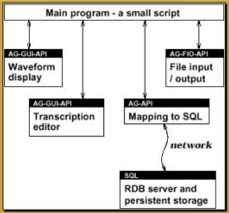
Figure 1: Interactions Among Annotation Tools and the Annotation Server

Incorporating ODBC support in AGTK greatly facilitates data sharing and collaborative annotation. Different users may be granted different levels of access to the server, e.g. to modify existing annotations, or just to add commentary to existing annotations (e.g. write a prose recommendation that a certain annotation be changed).

Annotation graph based annotation tools can also be tailored to permit certain categories of user to do certain kinds of edits. This supports annotation projects where there is a high degree of specialization amongst the geographically separated collaborators (e.g. if we were annotating discourse and intonation, and if junior annotators were given simple tasks, and senior annotators and researchers added their own specialized annotations, and checked the work of the junior annotators).

Updates may occur at various levels of granularity. For example, with record-level locking, two annotators could be working on the same annotation region without interfering with each other’s work. Section 4 also gives an example of how annotators can collaborate using column locking where different annotators are given different read/write permissions to edit certain annotation features.

So far we have focussed on collaborative annotation as the key benefit derived from moving to a relational database model. There are several other advantages as well.

With ODBC, an annotation application can access remote annotation servers. The user simply tells the application what annotation graph database on which server he/she wants to access by using an ODBC connect string which contains information of the name of the server, the name of the database, the user name and password. Note that the signal data does not need to reside in the same place as the annotation data. Distributed annotators may have local copies of large signal files while storing their annotations in a common central location.

While other annotation tools are able to store their annotations in a database [Cassidy, 1999], we are not aware of any projects which use this to support collaborative annotation.

We briefly note one final, significant benefit of storing all annotations in relational form. As Cieri and Bird ?) have discussed, many annotated recordings come with a variety of non-temporal data, such as speaker demographics, lexicons, and the like. These tables can be stored in relational form alongside the annotations, enabling us to integrate all of the data. Now, queries can perform joins across the temporal and atemporal data. For further discussion the reader is referred to [Cieri and Bird, 2001].

2.3. Exploiting the query language

In many annotation projects, the only way to view an annotation is with the same software that was used to create it. For any large annotation task – especially those involving collaboration – browsing individual annotations is usually not an efficient way to identify annotations requiring further work. The standard solution is to create special-purpose scripts which scan a collection of annotation files, opening the editor on each file which satisfies the user’s requirements.

Storing the annotations in a database is an obvious win since SQL queries can be used to efficiently identify the annotations requiring further attention. Such queries may even operate across multiple corpora. Unfortunately, SQL has some expressive limitations which render it unsuitable for certain kinds of query. For instance, we cannot express kleene closure over the annotation relation, since this requires a variable number of joins. However, regular expressions are a common feature of linguistic queries, and are heavily used in the special-purpose scripts (mentioned above).

In section 5 we will report the result of our experiments on pre-compiling the kleene closure so that these linguistically natural queries can be expressed. This work promises to greatly improve the flexibility of the annotation tools, permitting users to identify and load previously-created annotations according to complex criteria without leaving the annotation tool.

3. Relational Representation

This section discusses the database schema and the API that are used for storing and accessing a set of annotation graphs.

The design of the relational database schema is closely related to the AG library’s C++ implementation. Figure 2 depicts how AG library objects relate to each other. As the diagram shows, an AGSet is a collection of timelines and AGs. A timeline is a collection of signals. An AG contains multiple anchors and annotations. The annotation graph library objects also reference each other, for example, an annotation graph can reference a timeline; an annotation references two anchors (the start and end anchor); a Metadata object (’MD’ in the figure) could be referenced by an AGSet, AG, timeline or signal. There are also attributes associated with each library object, as shown in the picture. Please see [Maeda et al., 2002] for further details.

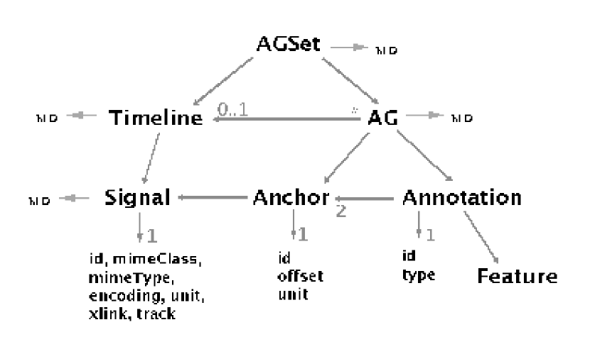
Figure 2: The Annotation Graph Object Model

3.1. Schema

The model described above is represented in a relational database as follows.

AGSET

Table AGSET stores attributes of all AGSets. XMLNS is the XML namespace of the ATLAS Interchange Format (AIF). XLINK specifies the XML Linking Language (XLink) specification the AGSet is using.

CREATE TABLE AGSET (
  AGSETID     VARCHAR(50) NOT NULL,
  VERSION     CHAR(10),
  XMLNS       CHAR(30),
  XLINK       CHAR(30),
  PRIMARY KEY (AGSETID))

AG

Table AG stores attributes of all AGs. AGSETID specifies the AGSet an AG belongs to. TIMELINEID indicates the timeline an AG is associated with. An AG can also have an optional type, indicated by TYPE.

CREATE TABLE AG (
  AGID        VARCHAR(50) NOT NULL,
  AGSETID     VARCHAR(50) NOT NULL,
  TIMELINEID  VARCHAR(50),
  TYPE        CHAR(10),
  PRIMARY KEY (AGID),
  FOREIGN KEY (AGSETID) REFERENCES AGSET)

TIMELINE

Table TIMELINE stores attributes of all timelines.

CREATE TABLE TIMELINE (
  AGSETID     VARCHAR(50) NOT NULL,
  TIMELINEID  VARCHAR(50) NOT NULL,
  PRIMARY KEY (TIMELINEID)
  FOREIGN KEY (AGSETID) REFERENCES AGSET)

SIGNAL

Table SIGNAL keeps attributes of all signals. AGSETID and TIMELINEID specify the AGSet and timeline a signal belongs to.

CREATE TABLE SIGNAL (
  AGSETID     VARCHAR(50) NOT NULL,
  TIMELINEID  VARCHAR(50) NOT NULL,
  SIGNALID    VARCHAR(50) NOT NULL,
  MIMECLASS   VARCHAR(50),
  MIMETYPE    VARCHAR(50),
  ENCODING    VARCHAR(50),
  UNIT        VARCHAR(50),
  XLINKTYPE   VARCHAR(50),
  XLINKHREF   VARCHAR(50),
  TRACK       VARCHAR(50),
  PRIMARY KEY (SIGNALID),
  FOREIGN KEY (AGSETID) REFERENCES AGSET,
  FOREIGN KEY (TIMELINEID) REFERENCES TIMELINE)

ANNOTATION

Table ANNOTATION keeps attributes of all annotations. AGSETID and AGID specifies the AGSet and the AG an annotation belongs to. STARTANCHOR and ENDANCHOR are the IDs of the start anchor and end anchor of the annotation. An annotation also has an type.

CREATE TABLE ANNOTATION (
  AGSETID      VARCHAR(50) NOT NULL,
  AGID         VARCHAR(50) NOT NULL,
  ANNOTATIONID VARCHAR(50) NOT NULL,
  STARTANCHOR  VARCHAR(50),
  ENDANCHOR    VARCHAR(50),
  TYPE         VARCHAR(50),
  PRIMARY KEY (ANNOTATIONID),
  FOREIGN KEY (AGID) REFERENCES AG,
  FOREIGN KEY (AGSETID) REFERENCES AGSET)

ANCHOR

Table ANCHOR stores attributes of all anchors. AGSETID and AGID specify the AGSet and the AG an anchor belongs to. OFFSET is the offset of an anchor. UNIT specifies the unit for the offset. SIGNALS indicates the signals that an anchor refers to.

CREATE TABLE ANCHOR (
  AGSETID     VARCHAR(50) NOT NULL,
  AGID        VARCHAR(50) NOT NULL,
  ANCHORID    VARCHAR(50) NOT NULL,
  OFFSET      FLOAT,
  UNIT        VARCHAR(50),
  SIGNALS     VARCHAR(50),
  PRIMARY KEY (ANCHORID),
  FOREIGN KEY (AGID) REFERENCES AG,
  FOREIGN KEY (AGSETID) REFERENCES AGSET)

METADATA

Table METADATA stores all the metadescriptions for AGSet, AG, Timeline and Signal. ID could be AGSETID, AGID, TIMELINEID or SIGNALID. These metadescriptions could use the Dublin Core elements to identify the title, creator and date of the work, and to give a prose description of its contents. For more discussion of the use of metadata for describing language resources, see [Bird and Simons, 2001].

CREATE TABLE METADATA (
  AGSETID     VARCHAR(50) NOT NULL,
  AGID        VARCHAR(50),
  ID          VARCHAR(50) NOT NULL,
  NAME        VARCHAR(50) NOT NULL,
  VALUE       TEXT,
  PRIMARY KEY (ID,NAME),
  FOREIGN KEY (AGSETID) REFERENCES AGSET)

Note that some values of the above tables, such as AGSETID, are stored redundantly to enable efficient loading. For example, this permits all the anchors of an AGSet can be loaded in a single query, which cannot be done if AGSETID is not stored in the ANCHOR table.

Feature Tables

AGTK also creates a feature table for each corpus. Each column of the feature table represents one possible feature of an annotation. The name of the column is the feature name and its value is the feature value. For example, to represent features of corpus ABC with possible feature names GENDER, AGE and POB (place of birth), AGTK creates the following table:

CREATE TABLE ABC (
  ANNOTATIONID VARCHAR(50) NOT NULL,
  GENDER      TEXT,
  AGE         TEXT,
  POB         TEXT,
  PRIMARY KEY (ANNOTATIONID),
  FOREIGN KEY (ANNOTATIONID) REFERENCES ANNOTATION)

Since an application can add or remove annotation features, AGTK must add or remove columns in the corresponding feature table. AGTK takes care of this when storing data back to the server, i.e. it changes the structure of the table if necessary before it stores annotation data back to the feature table.

3.2. AG database API

The AG database interface provides load and store functions.

LoadFromDB

void LoadFromDB(string connStr, AGSetId agsetId);

LoadFromDB loads the specified AGSet from the database server to memory. The variable connStr specifies the connection string that ODBC uses to connect to the server. It contains information such as hostname, database name, user name, and password.

Table 1 shows some of the parameters used in a connect string, for a complete list, see [http://www.mysql.com/doc/M/y/MyODBC_connect_parameters.html].

ODBC connect string arguments	What the argument specifies
DSN	Registered ODBC Data Source Name.
SERVER	The hostname of the database server.
UID	User name as established on the server.
	SQL Server this is the login name.
PWD	Password that corresponds with the login name.
DATABASE	Database to connect to. If not given, DSN is used.

Table 1: Parameters in Connect String

DSN is the registered ODBC Data Source Name. It should be defined in the .odbc.ini file in user’s home directory. All other arguments can be either defined in the .odbc.ini file, or defined in the connect string itself. To gain access to most ODBC data sources, the user must provide a valid user ID and corresponding password. These values are initially registered by the database administrator. The following is a sample driver section for DSN “talkbank” in the configuration file for iODBC. To make explanation easier, line numbers are included. Note that UID and PWD become USER and PASSWORD in iODBC’s configuration file.

1  [talkbank]
2  Driver   = /usr/local/lib/libmyodbc.so
3  DSN      = talkbank
4  SERVER   = talkbank.ldc.upenn.edu
5  USER     = myuserid
6  PASSWORD = mypasswd
7  DATABASE = talkbank

Line 1 is the name of the driver section, “talkbank” (the user can have multiple driver sections in a single configuration file). Line 2 specifies which ODBC driver to use. Line 3 gives the name of the DSN, which is “talkbank”. Line 4 specifies the hostname of the machine on which the database server is running. Lines 5 and 6 give the user name and password for connecting to the server. Line 7 identifies the database server to connect to. With a complete .odbc.ini file such as the above, the connection string can be just DSN=talkbank;. If the user has not specified some of the arguments in the configuration file, say USER and PASSWORD, he/she can still specify them in the connect string:

DSN=talkbank;UID=myuserid;PWD=mypasswd;

StoreToDB

void StoreToDB(string connStr, AGSetId agSetId);

StoreToDB stores the specified AGSet to the database server. The variable connStr contains connection information as explained above.

4. Collaborative Annotation with TableTrans

In this section we describe a collaborative annotation need which has been presented to us, and how this need can be addressed using the TableTrans tool. The context is research by Robert Seyfarth, Dorothy Cheney and colleagues at the University of Pennsylvania on social behavior and vocal communication in nonhuman primates. These researchers make extended audio recordings of primate interactions, making detailed notes of the social context and physical environment. Later, they listen to the recordings and identify particular vocalizations of interest, noting their start and end times and classifying the call types. Observations may be dense, or very sparse with extended periods in which nothing is coded. Each observation is entered into a row of a spreadsheet, and rows may have upwards of a dozen columns, each covering a different aspect of the observation, e.g.: recording offsets, tape number, date, time, location, animal id, group id, context (foraging/predator), call type, signal quality, and comments. Each row may also contain quantities derived from the corresponding period of the signal, such as mean energy. In this way, many thousands of observations are coded. Quantitative analysis of these tables addresses research questions in behavioral ecology and language evolution.

Much of the coding task is relatively straightforward and does not require highly trained annotators. Working from a digitized recording and field notes, an annotator can convert tape counter numbers to millisecond offsets, and enter such fields as the tape number, date, time and location. This work is typically done at a digitization station; while tapes are being uploaded to disk, the annotator works on previously uploaded materials. The result is a set of spreadsheets in which each row corresponds to an extent of audio, but where certain columns are left empty.

In the original version of this process, annotation files would remain on the digitization station until the first round of annotation was complete, at which time they would be transferred to a specialist – usually the original field researcher – for further annotation. The specialist would fill in columns that require a greater degree of critical judgement, such as the call type. However, during the course of listening to hundreds of calls, the untrained annotator gradually learns to discriminate most call types, and can usefully make a first pass at annotating some of the specialized columns. Later, these can be reviewed and post-edited by the specialist.

The unfortunate consequence of this regime is that the collaboration between the annotator and the specialist requires copies of the annotations to be circulated (e.g. by email) and/or arranging meetings. Neither of these is an efficient way to quickly resolve the unpredictable questions that may arise (and hold up) the annotation process. In addressing this problem, we have added a new capability to the TableTrans tool [Bird et al., 2002] which enables the user to choose to store all of its annotations in a central database. The configurations for the trainee and specialist versions of the tool specify which columns are available for read-only access, and which columns are available for read-write access. Even if physically separated, both parties can review the same material, listen to the audio segments, and discuss judgements (e.g. by email or telephone). In this way, collaboration, training and quality control can be done remotely, while each person has full access to the up-to-date annotations. The tool is able to prevent unauthorized modification of read-only columns, and indicates these columns by shading (see Figure 3).

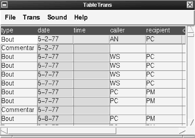
Figure 3: TableTrans With Read-Only Columns

This mode of collaborative annotation is possible because the data resides on a shared server, and because the tool can enforce a simple policy for the permission to edit particular spreadsheet columns.

5. Efficient AG Queries

Given that annotation graphs are stored in a relational database, it seems reasonable to use SQL for search. However, SQL turns out to be unsuitable for annotation graphs in terms of expressiveness and optimizability. Thus, a new query language for annotation graphs has been proposed [Bird et al., 2000]. In most cases, the new query language can be mapped into SQL. Therefore, it is still possible to utilize SQL and relational database technologies. There are a couple of advantages in this approach. First, given that we are taking full advantage of a relational database system, implementation is straightforward; we only need to map between query languages. Second, the optimization problem is reduced to the optimization of SQL queries, in which there is relatively little room for improvement.

The major problem in mapping between the proposed annotation graph query language and SQL is the arbitrary steps of arc tracing which cannot be expressed well in SQL. In this section, we propose a solution for the problem. Also, with a series of experiments, we probe the feasibility of this mapping approach in terms of efficiency which is critical in real time applications.

5.1. The experimental database

For the experiment, we set up a test database on a Linux PC running at 500 MHz. PostgreSQL [PostgreSQL Global Development Group, 2002] was used for the relational database. For test data, a part of the TIMIT corpus [Garofolo et al., 1986] was used, consisting of 1,680 TIMIT speech annotations. The contents of the database are summarized in the following table:

Object	Count
Agset	1
Ag	1,680
Annotation	80,378
txt	1,680
wrd	14,553
phn	64,145
Anchor	67,375

5.2. AG query example

Consider the following annotation graph query against our test database:

1. Query 1. Find word arcs whose phonetic transcription starts with a ‘hv’ and contains a ‘dcl’.

This query can be depicted by an annotation graph pattern as shown in Figure 4. It matches any wrd annotation that starts at anchor $X$ and ends at anchor $Y$ such that there exist a phn annotation labeled ‘hv’ that starts at anchor $X$ and ends at anchor $A$, a phn annotation labeled ‘dcl’ that starts at anchor $B$ and ends at anchor $C$, paths $A\leadsto B$ and $C\leadsto Y$ of phn annotations.

Figure 4: Annotation graph pattern for query 1.

This pattern can be written as follows using annotation graph query syntax:

    X.[].Y <- db/wrd
    X.[:hv].[]*.[:dcl].[]*.Y <- db/phn

Here is a complete annotation graph query for query 1.

    SELECT I
    WHERE  X.[id:I].Y <- db/wrd AND
           X.[:hv].[]*.[:dcl].[]*.Y <- db/phn;

Note that id:I is added to the pattern to select ids of matched annotations. Also note that there is no direct mapping to SQL for the above query because of the paths of phn annotations. The solution for this problem is discussed in the following sections.

5.3. $K^{*}$: Transitive closure of annotations

$K^{*}$ is a table containing connectability information between anchors. For example, if there is a path from anchor $A$ to anchor $B$ following annotations of type $t$, $K^{*}$ should contain a tuple $(A,B,t)$, and vice versa. The schema for $K^{*}$ is shown below:

CREATE TABLE Kstar (
  StartAnchor  VARCHAR(50),
  EndAnchor    VARCHAR(50),
  Type         VARCHAR(20),
  PRIMARY KEY (StartAnchor,EndAnchor,Type),
  FOREIGN KEY (StartAnchor,EndAnchor) REFERENCES Anchor);

Precomputing $K^{*}$, the transitive closure of annotations, eliminates the mapping problem. In fact, query 1 is now translated to SQL in Figure 5.

SELECT W.annotationid

FROM  (SELECT AnnotationId, StartAnchor, EndAnchor
       FROM   Annotation
       WHERE  Type=’wrd’) AS W,

      (SELECT StartAnchor, EndAnchor
       FROM   Annotation A, TIMIT F
       WHERE  A.Type=’phn’ AND
              A.AnnotationId=F.annotationId AND
              F.Label=’hv’) AS P1,

      (SELECT StartAnchor, EndAnchor
       FROM   Annotation A, TIMIT F
       WHERE  A.Type=’phn’ AND
              A.AnnotationId=F.annotationId AND
              F.Label=’dcl’) AS P2,

      (SELECT StartAnchor, EndAnchor
       FROM   Kstar
       WHERE  Type=’phn’) AS K1,

      (SELECT StartAnchor, EndAnchor
       FROM   Kstar
       WHERE  Type=’phn’) AS K2

WHERE  W.StartAnchor=P1.StartAnchor AND
       P1.EndAnchor=K1.StartAnchor AND
       K1.EndAnchor=P2.StartAnchor AND
       P2.EndAnchor=K2.StartAnchor AND
       K2.EndAnchor=W.EndAnchor
;

Figure 5: SQL query for query 1.

Domain Restriction

In the query in Figure 5, $K^{*}$ tuples of type phn are used. This is wasteful because it allows irrelevant anchors to be considered in the computation. For example, for two connected anchors, the SQL query will take those anchors into consideration as long as they are connected by phn annotations, even though they belong to different words.

To avoid this problem, we can restrict the domain of computation of transitive closure. In the above case, we can compute the transitive closure only for the phn annotations that belong to the same word. This will make the size of $K^{*}$ much smaller, making queries faster. The following table shows statistics for $K^{*}$ for the test database. The transitive closures are computed for wrd and phn annotations and for phn annotations within the wrd domain, denoted by phn/wrd.

Type	Count
wrd	91,960
phn	1,423,134
phn/wrd	271,323
Total	1,786,417

The following queries are variations of query 1.

1. Query 2. Find word arcs whose phonetic transcription starts with a ‘hv’:

   SELECT I
   WHERE  X.[id:I].Y <- db/wrd
          X.[:hv].[]*.Y <- db/phn;
   

2. Query 3. Find word arcs whose phonetic transcription starts with a ‘hv’ and ends with a ‘ix’:

   SELECT I
   WHERE  X.[id:I].Y <- db/wrd
          X.[:hv].[]*.[:ix].Y <- db/phn;
   

3. Query 4. Find word arcs whose phonetic transcription contains a ‘dcl’:

   SELECT I
   WHERE  X.[id:I].Y <- db/wrd
          X.[]*.[:dcl].[]*.Y <- db/phn;
   

The following table shows the performance of those queries and the effect of domain restriction.

Query	phn	phn/wrd
1	2.22	1.59
2	0.85	0.79
3	2.40	2.41
4	22.70	3.90

Since $K^{*}$ is a huge table, it is expected that queries with many references to $K*$ will suffer from the size of $K^{*}$. In considering this issue, suppose that we have the following general pattern for an annotation graph query:

    X.[].Y <- db/wrd
    X.[:l1].[]*.[:l2].[]*......[:ln].[]*.Y <- db/phn

The pattern has $n$ phn annotations and each pair of phn annotations has an intervening $K^{*}$ reference, a total of $n$ $K^{*}$ references. Figure 6 shows how the performance scales as the number of $K^{*}$ references increases. With 5 $K^{*}$ references, it took 23 hours and 40 minutes with a lot of memory swapping.

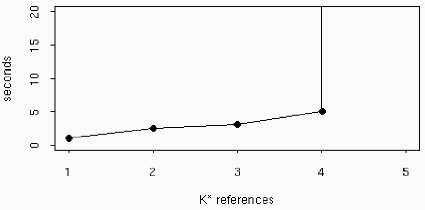
Figure 6: Long joins with $K^{*}$.

5.4. $K^{*}-$array: Alternative to $K^{*}$

$K^{*}$ shows poor performance when the query contains large number of $K^{*}$ references. In this section, we propose an alternative to $K^{*}$ to solve the problem.

Consider a boolean $n\times n$ matrix, where $n$ is the number of anchors in an annotation graph. We require a distinct matrix for each type $t$. The value of cell $(i,j)$ is true iff there is a path from anchor $i$ to anchor $j$ following annotations of type $t$. In general, the number of matrices required for an annotation graph is $N_{t}$ (number of annotation types) + $N_{d}$ (number of domain restrictions). Therefore, if tuples have a matrix as their attribute, the size of the $K^{*}$ table can be reduced to ($N_{t}$+$N_{d}$) $\times$ (number of annotation graphs).

A table is built as described above, using PostgreSQL’s array data type, and we call it $K^{*}-$array. The schema is shown below:

CREATE TABLE Kstar (
  AGId         VARCHAR(50),
  A            BOOL[][],
  Type         VARCHAR(20),
  PRIMARY KEY (AGId, Type),
  FOREIGN KEY (AGId) REFERENCES AG);

The size of $K^{*}-$array for our test database is 5,040; remember the size of $K^{*}$ is 1.8 million. Note that $K^{*}-$array reduces not only the size of the table but also the number of joins. For instance, Figure 7 is the $K^{*}-$array version of the SQL query in Figure 5, where two connectability tests are done by one $K^{*}-$array join. (anchor_num() is a function to map anchor ids to a natural number.) We can expect that this will improve performance for queries involving a large number of joins.

SELECT W.annotationid

FROM  (SELECT AnnotationId,StartAnchor,EndAnchor,AGId
       FROM   Annotation
       WHERE  Type=’wrd’) AS W,

      (SELECT StartAnchor, EndAnchor
       FROM   Annotation A, TIMIT F
       WHERE  A.Type=’phn’ AND
              A.AnnotationId=F.annotationId AND
              F.Label=’hv’) AS P1,

      (SELECT StartAnchor, EndAnchor, AGId
       FROM   Annotation A, TIMIT F
       WHERE  A.Type=’phn’ AND
              A.AnnotationId=F.annotationId AND
              F.Label=’dcl’) AS P2,

      (SELECT AGId, A
       FROM   Kstar_array
       WHERE  Type=’phn’) AS K

WHERE  W.StartAnchor=P1.StartAnchor AND
       K.AGId=W.AGId AND
       P2.AGId=W.AGId AND
       K.A[anchor_num(P1.EndAnchor)][anchor_num(P2.St artAnchor)] AND
       K.A[anchor_num(P2.EndAnchor)][anchor_num(W.End Anchor)]
;

Figure 7: SQL query for query 1 with $K^{*}-$array.

The following table shows the effect of the $K^{*}-$array for queries 1-4. There are clearly time savings, although there is little benefit from domain restriction.

	$K^{*}$		$K^{*}-$array
Query	phn	phn/wrd	phn	phn/wrd
1	2.22	1.59	1.24	1.24
2	0.85	0.79	0.57	0.57
3	2.40	2.41	2.40	2.40
4	22.70	3.90	2.42	2.24

Figure 8 demonstrates that the $K^{*}-$array can handle queries having a large number of joins.

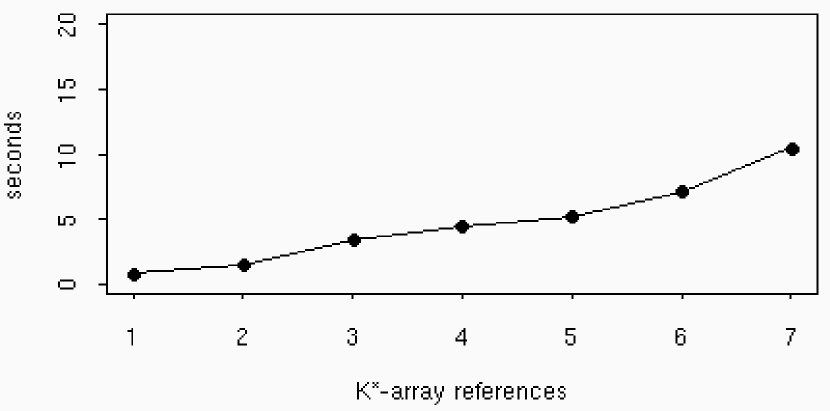
Figure 8: Long joins with $K^{*}-$array.

5.5. Future work

The result of these experiments shows that this approach to implementing annotation query is quite promising. There are, however, remaining tasks to complete the implementation. Tasks include: (i) implementation of translator (or mapper) from annotation graph query to SQL, (ii) further experimentation on vertical queries to allow efficient search on hierarchical information between annotations such as inclusion and overlapping, and (iii) specifying details of the query language syntax.

6. Conclusion

This paper has reported on models and tools for collaborative annotation based on annotation graphs. Annotation graphs are an extremely general and versatile data model for representing all kinds of annotation data. Moreover, they can be stored in a relational database and accessed remotely. The Annotation Graph Toolkit supports connections to ODBC-compliant database servers, making it easy for developers to create annotation tools that store all their data in a server. Apart from the obvious benefits for data management, this storage method opens up new possibilities for collaborative annotation, as reported above. We hope to have shown that it is completely straightforward to support a variety of different levels of collaborative annotation with existing AGTK-based tools, with a minimum of additional programming effort.

References

- Bird and Liberman, 2001 S. Bird and M. Liberman. 2001. A formal framework for linguistic annotation. Speech Communication, 33:23–60.
- Bird and Simons, 2001 S. Bird and G. Simons. 2001. The OLAC metadata set and controlled vocabularies. In Proceedings of ACL/EACL Workshop on Sharing Tools and Resources for Research and Education. http://arXiv.org/abs/cs/0105030.
- Bird et al., 2000 S. Bird, P. Buneman, and W.-C. Tan. 2000. Towards a query language for annotation graphs. In Proceedings of the Second International Conference on Language Resources and Evaluation. Paris: European Language Resources Association.
- Bird et al., 2002 S. Bird, K. Maeda, X. Ma, H. Lee, B. Randall, and S. Zayat. 2002. Tabletrans, multitrans, intertrans and treetrans: Diverse tools built on the annotation graph toolkit. In Proceedings of the Third International Conference on Language Resources and Evaluation.
- Cassidy, 1999 S. Cassidy. 1999. Compiling multi-tiered speech databases into the relational model: experiments with the Emu system. In Proceedings of the 6th European Conference on Speech Communication and Technology. http://www.shlrc.mq.edu.au/emu/eurospeech99.shtml.
- Cieri and Bird, 2001 C. Cieri and S. Bird. 2001. Annotation graphs and servers and multi-modal resources: Infrastructure for interdisciplinary education, research and development. In Proceedings of ACL/EACL Workshop on Sharing Tools and Resources, pages 23–30. Somerset, NJ: Association for Computational Linguistics.
- Garofolo et al., 1986 J. S. Garofolo, L. F. Lamel, W. M. Fisher, J. G. Fiscus, D. S. Pallett, and N. L. Dahlgren. 1986. The DARPA TIMIT Acoustic-Phonetic Continuous Speech Corpus CDROM. NIST. http://www.ldc.upenn.edu/Catalog/LDC93S1.html.
- Maeda et al., 2002 K. Maeda, S. Bird, X. Ma, and H. Lee. 2002. Creating annotation tools with the annotation graph toolkit. In Proceedings of the Third International Conference on Language Resources and Evaluation.
- PostgreSQL Global Development Group, 2002 PostgreSQL Global Development Group. 2002. PostgreSQL v7.2. http://www.postgresql.org/.