Active Virtual Network Management Prediction: Complexity as a Framework for Prediction, Optimization, and Assurance

Abstract

Research into active networking has provided the incentive to re-visit what has traditionally been classified as distinct properties and characteristics of information transfer such as protocol versus service; at a more fundamental level this paper considers the blending of computation and communication by means of complexity. The specific service examined in this paper is network self-prediction enabled by Active Virtual Network Management Prediction. Computation/communication is analyzed via Kolmogorov Complexity. The result is a mechanism to understand and improve the performance of active networking and Active Virtual Network Management Prediction in particular. The Active Virtual Network Management Prediction mechanism allows information, in various states of algorithmic and static form, to be transported in the service of prediction for network management. The results are generally applicable to algorithmic transmission of information. Kolmogorov Complexity is used and experimentally validated as a theory describing the relationship among algorithmic compression, complexity, and prediction accuracy within an active network. Finally, the paper concludes with a complexity-based framework for Information Assurance that attempts to take a holistic view of vulnerability analysis.

Keywords: Active Virtual Network Management Prediction, Kolmogorov Complexity, Information Assurance and Active Networks.

1 . Introduction

Kolmogorov Complexity ($K(x)$) [14] is the optimal compression of string $x$. This incomputable, yet fundamental property of information has vast implications in a wide range of applications including system management and optimization [11, 12], security [3, 7], and bioinformatics. Active networks [4] form an ideal environment in which to study the effects of tradeoffs in algorithmic and static information representation because an active packet is concerned with the efficient transport of both code and data. A question active network application developers must answer is: “How can I best leverage the capabilities that active networks have to offer?”. Because the word “active” in active networks refers to the ability to dynamically move code and modify execution of components deep within the network, this typically leads to another question: “What is the optimal proportion of content for an active application that should be code versus data?”. A method for obtaining the answer to this question comes from direct application of Minimum Description Length (MDL) [16] to an active packet. Let $D_{x}$ be a binary string representing $x$. Let $H_{x}$ be a hypothesis or model, in algorithmic form, that attempts to explain how $x$ is formed. Later in this paper, we view $H_{x}$ as a predictor of $x$ in the analysis of Active Virtual Network Management Prediction. For now let us focus on developing a measure of the complexity of $x$. MDL states that the sum of the length of the shortest encoding of a hypothesis about the model generating the string and the length of the shortest encoding of the string encoded by the hypothesis will estimate the Kolmogorov Complexity of string $x$, $K(x)=K(H_{x})+K(D_{x}|H_{x})$. Note that error in the hypothesis or model must be compensated within the encoding. A small hypothesis with a large amount of error does not yield the smallest encoding, nor does an excessively large hypothesis with little or with no error. A method for determining $K(x)$ can be viewed as separating randomness from non-randomness in $x$ by “squeezing out” non-randomness, which is computable, and representing the non-randomness algorithmically. The random part of the string, i.e. the part remaining after all pattern has been removed, represents pure randomness, unpredictability, or simply, error. Thus, the goal is to minimize $l(H_{e})+l(D_{x}|H_{e})+l(E)$ where $l(x)$ is the length of string $x$, $H_{e}$ is the estimated hypothesis used to encode the string ($D_{x}$) and $E$ is the error in the hypothesis. The more accurately the hypothesis describes string $x$ and the shorter the hypothesis, the shorter the encoding of the string. A series of active packets carrying the same information are measured as shown in Figure  1. Choosing an optimal proportion of code and data minimizes the packet length. The goal is to learn how to optimize the combination of communication and computation enabled by an active network. Clearly, if $K(x)$ is estimated to be high for the transfer of a piece of information, then the benefit of having code within an active packet is minimal. On the other hand, if the complexity estimate is low, then there is great potential benefit in including it in algorithmic form within the active packet. When this algorithmic information changes often and impacts low-level network devices, then active networking provides the best framework for implementing solutions (a specific example of separating non-randomness from randomness, although not explicitly stated as such, can be found in predictive mobility management as discussed in [4, 15]. However, the optimization of code/data or computation/communication has an additional constraint, namely security. Complexity also plays a significant role in the analysis of potential vulnerability within a network as discussed later in this paper.

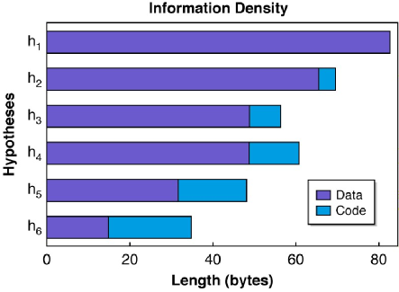
Figure 1: Algorithmic Content.

An active packet that has been reduced to the length of the best estimate of the Kolmogorov Complexity of the information it transmits will be called the minimum size active packet. When the minimum size active packet is executed to regenerate string $x$, the $D_{x}|H_{e}$ portion of the packet predicts $x$ using static data ($E$) to correct for inaccuracy in the estimated hypothesis. There are interesting relationships among Kolmogorov Complexity, prediction, compression and the Active Virtual Network Management Prediction (AVNMP) mechanism described in [4]. Details on the operation and mechanism of operation for AVNMP can be found in papers as early as [2]. Space limitations in this paper preclude a detailed description of operation, however, an overview of the characteristics and properties of AVNMP as well as new experimental results are presented and the relationships among complexity, predictability, and compressibility and information assurance are discussed and experimentally validated throughout this paper. The next section provides an overview of AVNMP before discussing its relationship to Kolmogorov Complexity. After required relevant background on AVNMP is explained, the relationship to Complexity Theory is developed beginning from a high level overview, then driving down into detailed relationships and experimental results.

2 . Active Virtual Network Management Prediction Overview

The Active Virtual Network Management Prediction (AVNMP) architecture provides a network prediction service that utilizes the capability of active networking to inject fine-grained models into the communication network to enhance network performance. Active Virtual Network Management Prediction (AVNMP) provides a network prediction service designed to facilitate the management of large, complex, active networks in a proactive manner. Network management includes a wide variety of responsibilities including configuration, fault, performance, accounting, and security management. A network management system must be able to monitor, control, and report upon the status of all these areas. In addition, the network management system should be more than a tool to generate reports and help fix problems, it should have the capability to anticipate and correct problems before they impact network performance. AVNMP accomplishes prediction and fault anticipation using a novel coupling of concepts from distributed simulation and active networking. A simple example demonstrating AVNMP results on a single node for load prediction is shown in Figure 2. In today’s management systems, a Management Information Base (MIB) maintains only current state values. In AVNMP, load is predicted into the future as real-time, called Wallclock, advances. Thus anticipated future values are available on the node as well as current values. In Figure 2, the Local Virtual Time (LVT) (future time), runs ahead of Wallclock Time (current time). Predicted load values are refined until Wallclock reaches the LVT of a particular value. This capability, described in detail in this paper, has been enabled by a new proactive network management framework combining three key enabling technologies; namely, distributed simulation, optimistic synchronization, and active networks.

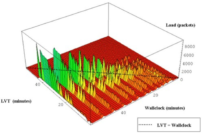
Figure 2: Convergence of Prediction and Reality in the AVNMP State Queue.

The predictive capability provided by AVNMP facilitates the development of a variety of predictive applications from mobile wireless location management and network security to improved QoS. AVNMP provides an ideal predictive service for mobile systems to predict their location [4]. Because mobile location can be predicted, hand-off situations are known ahead of time and setup for hand-off can take place prior to the hand-off event resulting in fast hand-off and improved QoS. In the domain of network security, AVNMP can anticipate the progress of an attack along most likely vulnerability paths and incorporate that information into decision-making. An attack can be propagated through the system before it actually occurs in order to determine its impact. In collaboration with the United States National Institute of Standards and Technology, AVNMP has been demonstrated with CPU prediction models showing the system’s ability to detect malicious active packets. Combined with the load prediction capability of AVNMP, Denial-of-Service attacks that use either abnormal amounts of CPU time or large numbers of small CPU packets can be detected and stopped [5]. With regards to QoS, the load application previously discussed allows resources and routing to be better managed by anticipating traffic in order to optimize load distribution within the network. A few additional selected uses for AVNMP are the ability to choose an optimum management polling interval that minimizes overhead based upon predicted rate of change and fault probability of the monitored data in a managed entity, fault correction before the system is impacted and with time available to perform dynamic optimization of repair parts, service, and solution entities such as software agent or human co-ordination and optimal resource allocation and planning not only for load, but also for CPU utilization that becomes significant in active networks. AVNMP allows “What if…?” scenarios to become an integral part of the network and finally, AVNMP-enhanced components are enabled with the ability to protect themselves by taking proactive, evasive action, such as migrating to safe hardware before anticipated disaster occurs.

A severe limitation of state-of-the-art network management techniques is that they are inherently reactive. They attempt to isolate the problem and determine solutions after the problem has occurred. Proactive management is a necessary ingredient for managing future networks. Part of the proactive capability is provided by analyzing current performance and predicting future performance based on likely future events and the network’s reaction to those events. This can be a highly dynamic, intensely computational operation. This has prevented management software from incorporating prediction capabilities. But distributed simulation techniques take advantage of parallel processing of information. If the management software can be distributed, it is possible to perform computation in parallel and aggregate the results to minimize computation overhead at each of the network nodes. The usefulness of optimistic techniques has been well documented for improving the efficiency of simulations. In optimistic logical process synchronization techniques, also known as Time Warp [2], causality can be relaxed in order to trade model fidelity for speed. If the system that is being simulated can be queried in real time, prediction accuracy can be verified and measures taken to keep the simulation in line with actual performance. AVNMP is implemented in an active network to provide predictive management of an active network. AVNMP is designed to utilize the additional processing and flexibility of an active network to provide better management of the added complexity in processing and bandwidth in an active network. AVNMP requires extreme network flexibility, primarily in the ability to inject fine-grained component models into the network. A much less flexible version of AVNMP could be implemented in legacy systems by building dedicated network component models directly into legacy network devices such as today’s routers. However, these models would be immobile and not easily updated or removed, most likely requiring the network device to be taken down when models are changed or updated. A better mechanism for using AVNMP to manage legacy networks would be to provide an active network overlay capable of monitoring legacy nodes. AVNMP should reside in the active network overlay providing a predictive management service for the legacy network. This has the added benefit of transitioning a legacy network to an active network.

AVNMP, injected into the network as an active application, is capable of modeling load and propagating state information in a manner that meets the demand for accuracy at a particular active node. Greater demand for prediction accuracy is met at the cost of AVNMP performance, that is, the ability of AVNMP to predict farther into the future. While this paper focuses on network traffic and load prediction, an AVNMP application to predict CPU utilization for active network in collaboration with National Institute of Standards and Technology [5, 9, 8] has been demonstrated. The inherently distributed nature of communication networks and the computational power unleashed by the active networking paradigm have been used to mutual benefit in the development of the Active Virtual Network Management Prediction mechanism. The active network benefits from AVNMP by continuously receiving information about potential problems before they occur.

AVNMP benefits from the active network in many ways. The first, and most practical way is the ease of development and deployment of this novel prediction mechanism. This could not have been accomplished so quickly or easily given today’s closed, proprietary network device processing. Another benefit is the fact that network packets now have the unprecedented ability to control their own processing. Great advantage was taken of this new capability in AVNMP. Virtual messages, varying widely in content and processing, can adjust their predicted values as they travel through the network. Finally, active networks add a level of robustness that cannot be found in today’s networks. This robustness is due to the ability of AVNMP system components, which are active packets, to easily migrate from one node to another in the event of failure –or the prediction of failure provided by AVNMP itself.

The desired characteristics of AVNMP are a large lookahead time, high prediction accuracy, low overhead and robust operation. Each of these characteristics is inter-related and a suitable tradeoff needs to be determined during configuration of the system. The AVNMP experimental validation configuration for the initial test discussed in this paper is a feed forward network consisting of a host containing the Driving Process and four intermediate active network nodes containing Logical Processes as shown in Figure 3. AH-1 and AH-2 are host nodes and AN-1 through AN-5 are active network nodes. The edges between the nodes represent links between the labeled ports on each node. All nodes are Sun Sparcs running the Magician active network execution environment. The AVNMP system parameters were configured as shown in Table 1. In this experiment AVNMP is predicting the packet input and output rate for each link at each node, from an application residing on AH-1 that is transmitting an active audio packets.

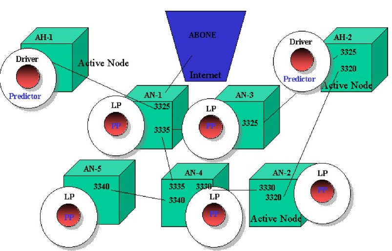
Figure 3: AVNMP Test Configuration.

Parameter	Value
Sliding Window Lookahead Length ($\Lambda$)	200 seconds
Virtual Message Generation Rate	0.5 virtual messages/millisecond
Virtual Message Prediction Step Size	20 seconds
Tolerance for Prediction Error ($\theta$)	500 Messages/second
Virtual Real Message Ratio	1 virtual/real message
Load Hypothesis ($H_{e}$)	Linear Extrapolation

Table 1: AVNMP Test Parameters.

The State Queue plot, Figure 2, shows the predicted traffic load values cached in the State Queue as a function of Local Virtual Time (LVT) and Wallclock. As Wallclock approaches any given Local Virtual Time, the predicted load values converge towards the actual load. The dashed line placed diagonally across the surface highlights where predicted time and actual time converge. The general operation is illustrated in the next five graphs where all measurements, unless otherwise indicated, are from node AN-4. These curves validate intuitive trends in the operation of AVNMP. Figure 4 shows the reduction in tolerance versus time that is pre-programmed into each Logical Process. The Y-axis is the tolerance that is demanded between the predicted value and the actual value of an Simple Network Management Protocol (SNMP) packet counter. This value is decreased purposely in this experiment in order to create a greater demand over time for accuracy and thus create a challenging validation of the AVNMP system under gradually increasing stress. In Figure 5 the proportion of out-of-tolerance messages is shown as a function of Wallclock. The Y-axis is the proportion of messages that arrived at a specific node out of tolerance, that is, the actual value exceeded the predicted value by an amount greater than the tolerance setting. As Wallclock progresses, the tolerance is purposely reduced causing a greater likelihood of messages exceeding the tolerance. This is done in order to validate the performance of the system as stress, in the form of greater demand for accuracy, is increased. Figure 6 shows the prediction error as a function of Wallclock. The Y-axis is the difference in the number of packets received versus the number of packets predicted to have been received. This graph verifies that the system is producing more accurate predictions as the demand for accuracy increases. However, the Y-axis of Figure 7 shows the lookahead decreasing versus Wallclock. The expected lookahead time is the difference between Wallclock and the Local Virtual Time at a particular node. The demand for greater accuracy reduces the distance into the future that the system can predict. Finally, in Figure 8, speedup, the ratio of virtual time to Wallclock of the real system, is shown as a function of Wallclock. The speedup is reduced as the demand for accuracy is increased. As previously mentioned, only for purposes of this experiment, the tolerance is being reduced as Wallclock progresses, causing the accuracy to increase while loosing performance in terms of speedup and lookahead.

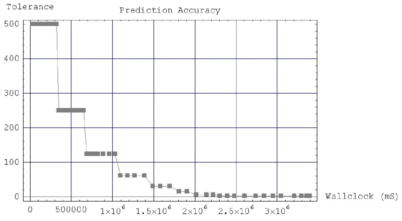
Figure 4: Tolerance Setting Decreases as Wallclock Increases Thus Demanding Greater Accuracy.

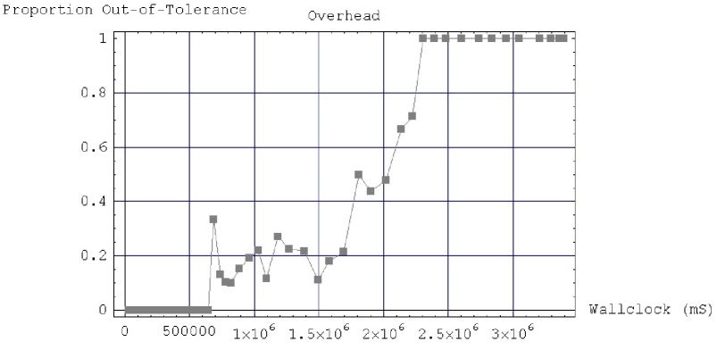
Figure 5: Demand for Greater Accuracy Causes the Proportion of Out-of-Tolerance Messages to Increase.

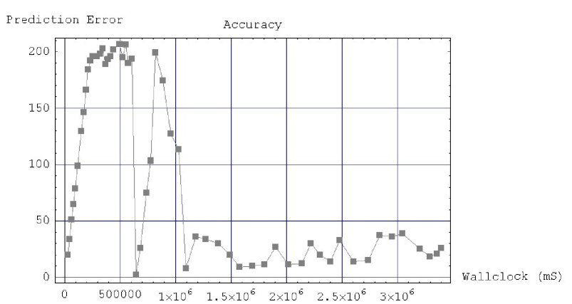
Figure 6: Predictions Become More Accurate…

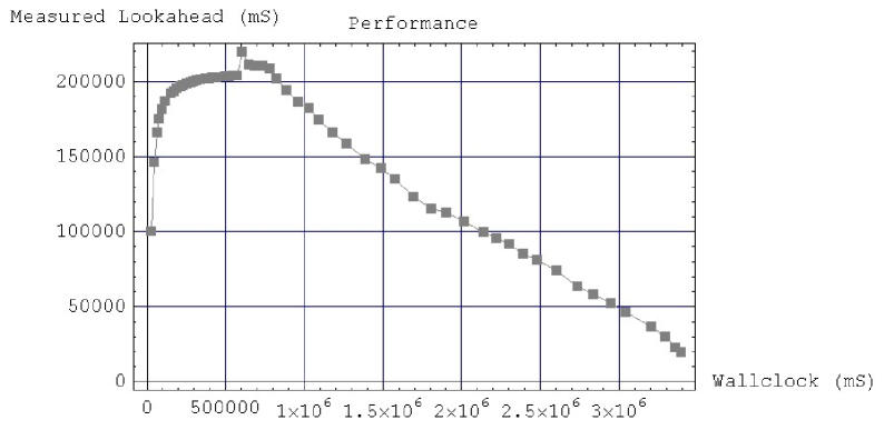
Figure 7: …at the Expense of Lookahead…

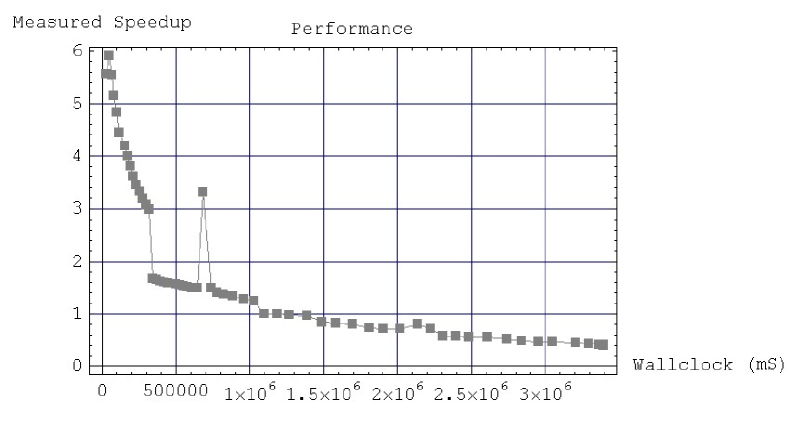
Figure 8: …and Speedup.

2.1 . AVNMP Overhead

AVNMP has the potential to generate two forms of overhead, processing overhead and bandwidth overhead. If the predicted results are within the user specified error tolerance and the user fully utilizes the predicted results, then overhead is at a minimum. The question of overhead versus benefit becomes one that depends upon the perceived utility of predictive capability and depends significantly upon the manner and application in which it is used. It is the author’s belief that load and processing prediction are of particularly great importance in an active network where routing is based upon not only load, but the processing capability required by active applications. In this section, the load prediction application example is continued with overhead results displayed in terms of processing time and number of packets transmitted. The expected Active Network Encapsulation Protocol (ANEP) [4] packet size measured during this test was 1000 bytes.

2.1.1 Task Execution Time and Message Overhead

The task execution time is the Wallclock time the system spends executing a non-rollback message. It was expected that task execution time would be essentially constant; however, it increases in direct proportion to the number of rollbacks as shown in Figure 9. This is caused by the lack of fossil collection. The increase in the number of values in the State Queue is causing access of the State Queue and Management Information Base (MIB) to slow in proportion to the queue size. Figure 10 displays the number of virtual messages versus Wallclock and Figure 11 displays the total number of anti-messages. This is expected to increase over time. This value is reset every time the tolerance is tightened (every 5 minutes in this case).

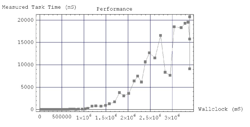
Figure 9: Expected Task Execution Time as a Function of Wallclock.

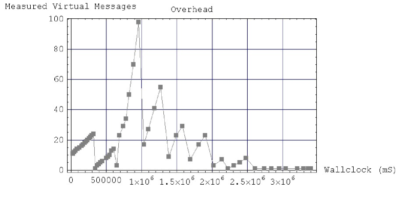
Figure 10: Number of Virtual Messages versus Wallclock.

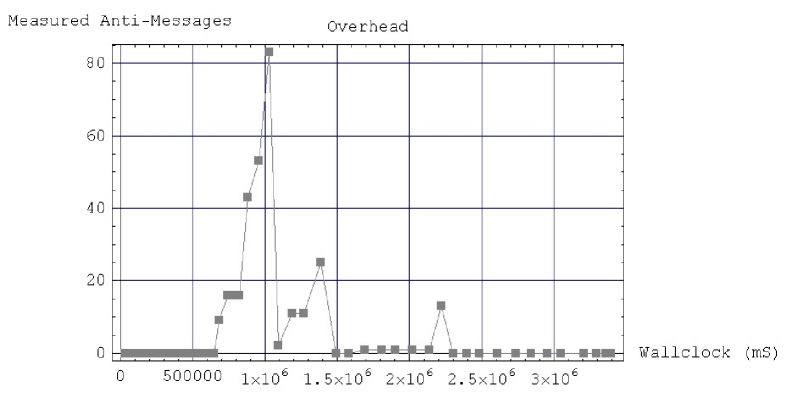
Figure 11: Number of Anti-Messages versus Wallclock.

2.2 . AVNMP Robustness

AVNMP is both an active application and an application whose purpose is to provide predictive management of other active applications. As a management application it must be robust in the presence of a failing environment. So far, it has shown to provide graceful predictive degradation in the presence of dropped packets and broken links. AVNMP consists of two main types of active packets: AvnmpLP, which is the Logical Process, and AvnmpPacket, which is the virtual message. If an AvnmpLP packet is dropped, the destination node will not have the capability to work forward in time or forward virtual messages. Thus, AVNMP features will not be available on the node for which AvnmpLP was destined and the accuracy of other nodes may be reduced. If an AvnmpPacket is dropped or unexpectedly delayed, accuracy will be reduced because the State Queues of downstream nodes will lack a predicted value. However, AVNMP will continue to operate with degraded performance. In the next section the role of complexity in understanding prediction is discussed. Ideally, of course, AVNMP should have predicted the error condition and taken action to mitigate it. However, control mechanisms have not yet been implemented.

2.3 . Networking Viewed Through the Lens of Complexity

AVNMP can provide early warning of potential problems; however, the identification of a solution and marshaling of automated solution entities within an active network has not yet been fully addressed. This project has begun to lay the groundwork for such automated composition of management solutions within an active network [4]. This direction is being carried forward by exploration of a relatively unexplored area -understanding the benefits of active networking, Algorithmic Information Theory, and its close companion, Complexity Theory. To our knowledge, this work is the first to propose and begin investigation into the newly available processing power of active networking through the concept of Complexity and Algorithmic Information (“Streptichrons”) as shown in Figure 12. Legacy networks, which are today’s passive networks, have been designed to optimize transmission of passive data using bit compression based upon the underlying notion of Shannon Entropy. AVNMP has shown that active networks allow for the possibility of executable models and that the corresponding information packets might be best studied with Kolmogorov Complexity as the underlying theory. It is serendipitous that Complexity Theory has been receiving more attention lately and is making significant theoretical progress at the same time that research into active networking is taking place. Active networks provide a new paradigm and enhanced capabilities, which, when combined with ideas from Algorithmic Information Theory [14], might lead to superior, innovative solutions to problems of network management. One possible approach proposes to combine Kolmogorov Complexity with the science of Algorithmic Information Theory (sometimes called Complexity Theory) to build self-managed networks that draw on fundamental properties of information to identify, analyze, and correct faults, as well as security vulnerabilities, in a distributed information system [11, 12]. Specifically, we suspect that complexity measures can be used to detect and analyze problems in a network, and to facilitate techniques to remedy network faults. We also envision that Kolmogorov Complexity can be applied directly to improve the performance of AVNMP. In general, complexity is not computable; however, the bounds on complexity tighten continuously as fundamental research in Kolmogorov Complexity progresses.

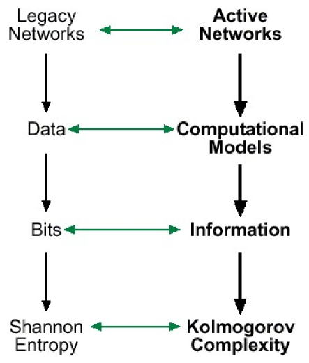
Figure 12: Active Networks and Legacy Networks as Viewed by AVNMP.

One potential drawback to AVNMP, gently pointed out earlier in this paper, is the fact that AVNMP itself consumes resources in an effort to predict resource usage in a network. Resource consumption by AVNMP is tied directly to accuracy: higher accuracy costs more in terms of bandwidth utilization, associated with simulation rollbacks and the concomitant transmission of anti-messages. Despite this relationship, potential exists to nearly reach the theoretical minimum amount of bandwidth to achieve maximal model accuracy. This possibility arises because AVNMP consists of many small, distributed models (each a description of a theory) that work together in an optimistic, distributed manner via message passing (data). Each AVNMP model can be transferred, using an active network, as a Streptichron [4], which is any message that contains an executable model in addition to data for prediction. Using Streptichrons, the optimal mix of data and model can be transmitted to implement MDL. Achieving maximal model accuracy at minimal bandwidth provides the best AVNMP accuracy at the least cost in AVNMP resource consumption.

Other possibilities exist to exploit Kolmogorov Complexity to improve AVNMP performance. For example, one can apply the MDL technique to the rollback frequency of all the AVNMP enhanced nodes in a network. A low rollback complexity (which suggests a high compressibility in the observed data) would indicate patterns in the rollback behavior that could be corrected relatively easily by tuning AVNMP parameters. High complexity (low compressibility) would indicate the lack of any computable patterns, and would suggest that little performance improvement could be achieved by simply tuning parameters. Thus, we hypothesize that our tuning gradient should be guided toward regions of high complexity, which suggests that we can tune parameters to improve the rollback frequency. The next section focuses upon experimental results relating prediction to complexity gathered from the operation of the AVNMP system.

2.4 . AVNMP and Kolmogorov Complexity

In AVNMP, information that impacts the network is transmitted based upon prediction at a low level within the network. Thus, AVNMP allows experimentation in defining the boundaries within which active networking is beneficial. In Figure 13 an active and passive form of AVNMP is represented. The passive case is represented in the upper portion of the figure. In the passive case, actual data ($D_{x}$) is observed at the Driving Process. Note that in the AVNMP architecture, Driving Processes exist at the edge of the system. They monitor external forces acting upon the system, such as load, and generate virtual messages, which are a short-term local prediction about a specific property such as input load, that are injected into the AVNMP system. The Driving Process has a hypothesis that has been formed about the data; predicted data ($D_{y}$) is generated in the form of static virtual messages. The term static indicates that information content within the message contains no executable code. The virtual messages are propagated through the network driving the the system ahead of Wallclock. When error in the hypothesis exceeds a preset threshold, AVNMP causes rollbacks to occur in order to adjust for the inaccuracy. In the lower portion of Figure 13, the hypothesis is included within each packet and is used to encode $D_{y}$ within the code portion of the active packet.

Figure 13: Active versus Passive Form of AVNMP.

What is the relationship between the estimated operating hypothesis ($H_{e}$) that can encode an AVNMP packet and $H_{e}$ as the predictor in the Driving Processes? First, they are the same hypothesis. Second, it has been shown [14] that the shorter the packet, the better the predictor. Conversely, the worse the prediction, the longer the $E$ value, where $E$ can be considered any of the following equivalent names: error, complexity, or randomness within the AVNMP packet encoding. Can Active Virtual Network Management Prediction benefit from the fact that the smallest algorithmic form is also the most likely predictor of a sequence? This can come about because Driving Processes and Streptichrons (active virtual messages anticipating events in the future) benefit by being both small and accurate as shown in Figure 14. The objective is to increase the rate of convergence of the predictions held within the State Queue to converge to the actual value that will occur in the future, and to converge to that value before it actually exists. Actual and predicted values within a particular instance of a State Queue were shown in Figure 2. Let us examine AVNMP results in light of complexity in more detail in the next section.

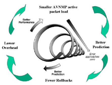
Figure 14: Better Prediction Implies Smaller Packets Implies Better AVNMP Performance Implies Better Prediction.

2.5 . Load Prediction And Complexity In Active Virtual Network Management Prediction

With regard to active packets and information theory, passive data is simple Shannon compressed data, and active packets are a combination of data and program code whose efficiency can be estimated by means of Kolmogorov Complexity. The active network Kolmogorov Complexity estimator is currently implemented as a quick and simple compression estimation method. It returns an estimate of the smallest compressed size of a string. It is based upon computing the entropy of the weight of ones in a string. Specifically it is defined in Equation 1 where $x\#1$ is the number of 1 bits and $x\#0$ is the number of 0 bits in the string whose complexity is to be determined. Entropy is defined in Equation 2. See [6] for other measures of empirical entropy and their relationship to Kolmogorov Complexity. The expected complexity is asymptotically related to entropy as shown in Equation 3.

$$\hat{K}(x)=l(x)H({{x\#1}\over{x\#1+x\#0}})+\log_{2}(l(x))$$ (1)

$$H(p)=-p\log_{2}p-(1.0-p)\log_{2}(1.0-p)$$ (2)

$$H(X)=\sum_{l(x)=n}P(X=x)K(x)$$ (3)

Load prediction data sampled from execution of AVNMP is analyzed relative to several hypotheses. The goal is to use a simple example to demonstrate the relationship among accuracy of hypotheses, complexity, and compression. The initial hypothesis ($H_{e}$) (regardless of naivete in choice of hypothesis) is that the data can be characterized by a simple linear extrapolation based upon the last sampled load values. This is shown in Figure 15 where the gray boxes are actual load samples and the black stars are predicted load samples. Note that the predicted load is based upon a short history shown in the graph as the initial match between predicted and actual load.

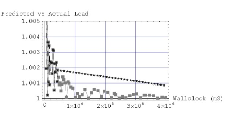
Figure 15: Prediction Hypothesis ($H_{e}$) Compared with Actual Load in AVNMP Test.

Various enhancements are added to the initial hypothesis to create new hypotheses for our test. In this specific case, a running average was used to smooth the data before the extrapolation. The size of the running average defines a hypothesis. Each enhancement is considered a new hypothesis ($H_{e}$) in this experiment. In Figure 16, for each $H_{e}$ the sum of the error in predictions is graphed as the gray boxes in the lower portion of the graph. The compressed size of the corresponding error is plotted as the black stars in the upper portion of the figure. Clearly a better hypothesis concerning the origination of the data results in better prediction and greater compression, while poor hypotheses result in inaccurate prediction and reduced compression. This provides a concrete demonstration of the relation between complexity and prediction accuracy.

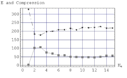
Figure 16: Prediction Error and Complexity Estimate over a Range of AVNMP Hypotheses for Load Prediction.

A key contribution presented in this paper is the hypothesis and supporting experimental validation that greater complexity results in greater prediction error, and thus greater likelihood of AVNMP rollback. Load prediction error from AN-1 (see the experimental configuration shown in Figure 3) within the network is compared with the estimated complexity of the actual load. In Figure 17 the load prediction error is plotted with the estimated complexity versus Wallclock where values are taken over intervals of the same length as the Sliding Lookahead Window shown in Table 1. Larger error, and thus more likely rollback, occurs during periods of relatively high complexity, while complexity is low during periods of low prediction error.

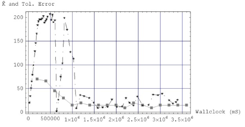
Figure 17: Estimated Complexity and Error within AVNMP.

As predictions become more inaccurate in AVNMP, virtual messages should slow down, rather than burden the system with potential rollbacks. Poorly predicted messages will naturally be larger in their minimum size, which slows down their rate of propagation in proportion to their inaccuracy.

Another issue concerns a mechanism for feedback to the Driving Process in order to improve $H_{e}$. Such a feedback mechanism can be based upon input from the complexity estimate, or minimum encoded packet size, of virtual messages. The hypothesis is adjusted in a manner that drives the system towards minimizing encoded virtual message size.

3 . Complexity and Assurance

Complexity is useful not only for management prediction and active packet length optimization, but also for security. The vulnerability analysis technique presented in this section takes into account the innovation of an attacker. A metric for innovation is not new; 700 years ago William of Occam suggested a technique [10]. The salient point of Occam’s Razor and complexity-based vulnerability analysis is that the better one understands a phenomenon, the more concisely the phenomenon can be described. This is the essence of the goal of science: to develop theories that require a minimal amount of information to be fully described. Ideally, all the knowledge required to describe a phenomenon can be algorithmically contained in formulae, and formulae that are larger than necessary lack of a full understanding of the phenomenon. Consider an attacker as a scientist trying to learn more about his environment, that is, the target system. Parasitic computing [1] is a literal example of a scientist studying the operation of a communication network and utilizing it to his advantage in an unintended manner. In Parasitic computing, checksums, additional overhead supposedly designed to insure the integrity of the information, are turned against the system and used to the attacker’s advantage. In fact, because information assurance safeguard developers do not yet have a comprehensive conceptual framework in which to evaluate the effectiveness of their safeguards individually or as composites of safeguards, such scenes are unfortunately all too common. Safeguard designers must be able to capture and quantify the mechanism by which an attacker as scientist generates hypotheses and theorems about a system under attack. Theorems are attempts to increase understanding of a system by assigning a cause to an event, rather than assuming all events are randomly generated. If theorem $x$, described in bits, is of length $l(x)$, then a theorem of length $l(m)$, where $l(m)$ is much less than $l(x)$, is not only much more compact, but also $2^{l(x)-l(m)}$ times more likely to be the actual cause than pure chance [10]. Thus, the more compactly a theorem can be stated, the more likely the theorem is to be correct. A measure of this compactness is described and utilized in more detail later in this paper.

Imagine a vulnerability identification process that consists of the following: waiting for an information system to be attacked, then, assuming it survives and one can detect the attack, analyzing the attack, and if the information system is still not compromised, adding this information to one’s knowledge base. This technique would be unacceptable to most people, but it is essentially the technique used today. Information assurance, and vulnerability analysis in particular, are hard problems primarily because they involve the application of the scientific method by a defender to determine a means of evaluating and thwarting the scientific method applied by an attacker. This self-reference of scientific methods would seem to imply a non-halting cycle of hypothesis and experimental validation being applied by both offensive and defensive entities, each affecting the operation of the other. Information assurance depends upon the ability to discover the relationships governing this cycle and then quantifying and measuring the progress made by both an attacker and defender. The salient factor controlling the paths taken by attacker and defender are governed by the complexity of the system. Whether such properties are measurable and how they will behave in a complex system is a topic of open debate. However, a metric and framework are required for quantifying information assurance in such an environment of escalating knowledge and innovation. Progress in vulnerability analysis and information assurance research cannot proceed without fundamental metrics. The metrics should identify and quantify fundamental characteristics of information in order to guarantee assurance.

A fundamental definition of vulnerability analysis is formulated in this paper based upon attacker and defender as reasoning entities, capable of innovation. Truly innovative implementations of attack and defense lead to the evolution of complexity in an information system. Understanding the evolution of complexity in a system enables a better understanding of where to measure and how to quantify vulnerability and leads towards a calculus of information complexity. The design and implementation of a complexity-based vulnerability analysis technique is under development as a tool for automated measurement of information assurance. The motivation for complexity-based vulnerability analysis comes from the fact that complexity is a fundamental property of information and can be ubiquitously applied. The presentation and analysis of the Kolmogorov Complexity-based vulnerability analysis framework must accomplish several goals. As initially stated, the vulnerability analysis technique must demonstrate the ability to account for the innovation of an attacker. The technique should be based upon fundamental properties of information, rather than suffer from the combinatorial explosion that occurs when explicitly examining all possible events generated by specific systems. The vulnerability results should make intuitive sense; vulnerability is reduced by increasing the apparent complexity of access to information from potential attackers while increasing vulnerability for less complicated, or in some sense shortest paths of access to information. A topological view of vulnerability can be demonstrated. This is demonstrated by means of a Kolmogorov Complexity Map (K-Map) in which low complexity paths, which are likely to be easy for an attacker to follow, are identified. The concept of a K-Map, or complexity grid, is shown in Figure 18 and the K-Map for a specific example is derived later in this paper and shown in Figure 29. Figure 18 may itself appear quite complex upon first glance; however, focus upon individual parts of the figure in a logical progression. Begin with the information to be protected that lies at the bottom of Figure 18. Attacks are illustrated as the thin downward-pointing arrows attempting to penetrate the system in order to manipulate the information. Numerous safeguards, supposedly designed to protect the information, each designed to mitigate particular types of attack, are shown as barriers with various levels of porosity inserted across the middle of the figure. The overall complexity of the system is illustrated by the surface contour located above the information and safeguards and is comprised of the complexity of several entities, namely: the information itself, the complexity of the system in which the information resides and the complexity of the safeguards. Innovative attacks will be more likely to successfully penetrate areas of low complexity, easier to comprehend components of the system. In addition, specific types of attacks, such as Distributed Denial of Service (DDoS) will appear as warps in the complexity grid. This is due the inherent system correlation in DDoS attack-streams. The vulnerability analysis technique should be applicable in a highly dynamic and amorphous information environment; an active network environment is chosen because information can be transmitted through an active network while its proportion of algorithmic content varies. In other words, static data or executable code or various combinations of both can represent information; both forms of information should have high assurance. The assurance of their interaction at a low level within an active network presents a nice challenge.

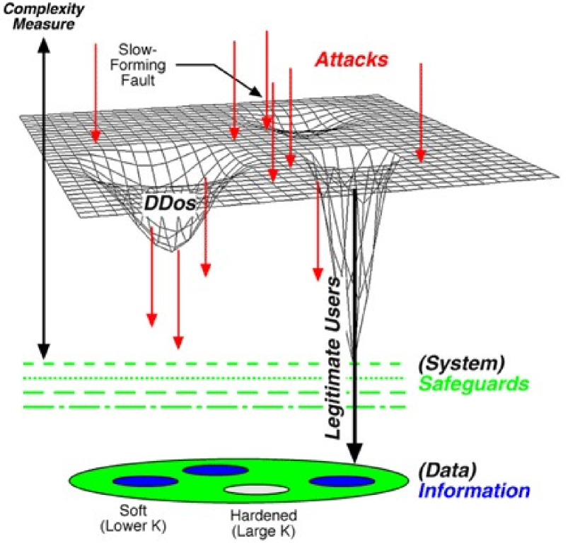
Figure 18: Conceptual Illustration of a Vulnerability and Attack Detection Complexity Grid.

Kolmogorov Complexity provides a measure of complexity that can be utilized for vulnerability analysis. Observe an input sequence at the bit-level and concatenate with an output sequence at the bit-level. This input/output concatenation is observed for either the entire system or for components of the system. Low complexity input/output observations quantify the ease of understanding by a potential attacker. Previous work has demonstrated the use of Kolmogorov Complexity for Distributed Denial of Service (DDoS) attack detection [13]. Definition 1 explicitly states the means of measuring the complexity of a system component, or protocol interaction, to a potential attacker.

Definition 1:Vulnerability Metric

Vulnerability is inversely proportional to $K(x[opstart:opend])/l(x[opstart:opend])$ where $opstart$ is the bit at which an operation to be discovered within an information system begins, and $opend$ is the last bit in an attacker’s observation.

In the remainder of the paper, excerpts from a Mathematica Notebook are included. The excerpts contain code using common mathematical and programming constructs and therefore should be intuitively obvious without requiring knowledge specific to Mathematica; any Mathematica specific details are explained in the text. As a specific example of the algorithmic capabilities of active networks, consider the transmission of an estimate of $\pi$. One could choose to send $\pi$ as an extremely large number of digits; in contrast, one could send a smaller algorithm capable of generating $\pi$ to an arbitrary number of digits. Consider an illustration of this concept in more detail. The Mathematica code, $\{\{\#1/\#2\&\}\},\{22.,7.\}\}$, represents an unnamed function that divides the first argument by the second argument; the function implements $22/7$. Consider that the function ($\{\{\#1/\#2\&\}\}$) and the data ($\{22.,7.\}$) remain unevaluated and are transmitted together. This represents an active packet; it contains part code and part data. The RUN function evaluates the function and returns the result; the result in this case is static data, a legacy data packet. Mathematica code that analyzes the characteristics of algorithmic and passive information transmission is shown in Figure 19. The active packet is defined as $\{\{\#1/\#2\&\}\},\{22.,7.\}\}$, which contains a pair of values and the code necessary to perform division. The legacy, or passive packet, is defined as $RUN\{\{\#1/\#2\&\}\},\{22.,7.\}\}$, which pre-computes the result of the division and transmits the same information in non-algorithmic form. The argument defined as $\{\{1,2,3,4\},\{4,3,2,1\}\}$ identifies the links traversed by the active and passive packets respectively. In this case, the first packet begins by crossing link one and the second packet begins by crossing link four. The argument defined as $\{100,100,1000,1000\}$ indicates link capacities for links one, two, three, and four. Thus, the first packet transmits both code and data that generates the intended information, while the second packet transmits raw data only. The result of executing the function below is load and processing time spent on each link and node for each packet. In Figure 20, the load induced by sending the estimate of $\pi$ using AnetSim in Figure 20 is plotted for each link. Clearly, the algorithmic representation of the information is more compact and used less link capacity. In fact, this reinforces the fact that, by knowing how to compute $\pi$, one could build a more compact representation; this demonstrates Occam’s Razor for a useful purpose, information compression. This has facilitated study of active (algorithmic) versus passive transmission of information. For example, we allow the ratio of data to code to change for the same information as the packet traverses the network in a manner that optimizes both link capacity and node processor speed.

Before continuing with a specific analysis, consider Figure 24 which shows a topological view of components of a sample system under analysis. The nodes are active application components and the links are security relationships between the components; the links are quantified using Kolmogorov Complexity-based vulnerability analysis. START is a state that is outside the system that represents the state of the system before it has been penetrated by an attacker.

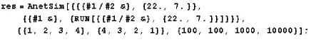
Figure 19: Algorithmic View of Active Packets.

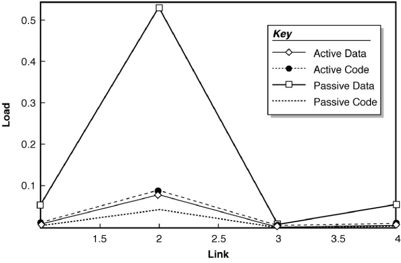
Figure 20: Algorithmic versus Static Active Network Information Load.

3.1 . Complexity Surface: The Kolmogorov Complexity Map

The General Electric Corporate Research and Development active network test bed implements complexity probes as part of the active execution environment. The choice was made to embed the complexity probe in the execution environment rather than as an active application because it is necessary to examine the content of active packets before they reach the execution environment. In the Mathematica simulation, each component of the active application contains probe-input points through which bit level input and output is collected. A complexity estimator based upon the simple inverse compression ratio from Equation 1 is used to estimate complexity in the density metric. Figure 21 graphs results from density estimates taken of accumulated input and output of three separate components of the active network application. The graph shows the complexity of bit-level input and output strings concatenated together. That is, every input sequence is concatenated with an output sequence and the density of the sequence is recorded at the bit-level. The input/output concatenation is generated either for individual components of the system of for a composition of components. If there is low complexity in the input/output observation pairs, then it is likely to be easy for an attacker to understand the system, as in Definition 1. The X-axis is the number of input and output observations concatenated to form a single string of bits. From Figure 21, it would appear that Component E is most vulnerable due to its consistently low complexity while Component B appears to be the least vulnerable due to its larger complexity. These results make intuitive sense because Component E simply forwards data without any form of protection while Component B adds noise to the data. This vulnerability method does not take into account whether a component reduces or increases complexity; in other words whether the change was endothermic or exothermic complexity. These results demonstrate how vulnerabilities are systematically discovered using complexity; vulnerabilities can be quantified to a value within the bounds of the complexity measure error.

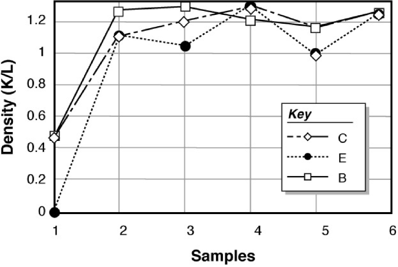
Figure 21: Component Complexity for Components B, C, and E.

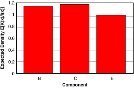
Figure 22: Mean Component Complexities for Components B, C, and E.

In order to develop the Kolmogorov Complexity Map (K-Map), consider the topology in more detail. Figure 23 shows the resulting densities inserted into a Mathematica graph object. The graph object allows graph theory related analyses to be applied. The directed graph in Figure 24 shows the relationship among the vulnerabilities. The START state, located in the center of the topology, represents a location outside the system. In Figure 25 a matrix is generated that shows the cost, in terms of complexity, of traveling from any node to any other node in the K-Map.

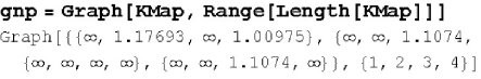
Figure 23: Kolmogorov Complexity Map (K-Map) Matrix.

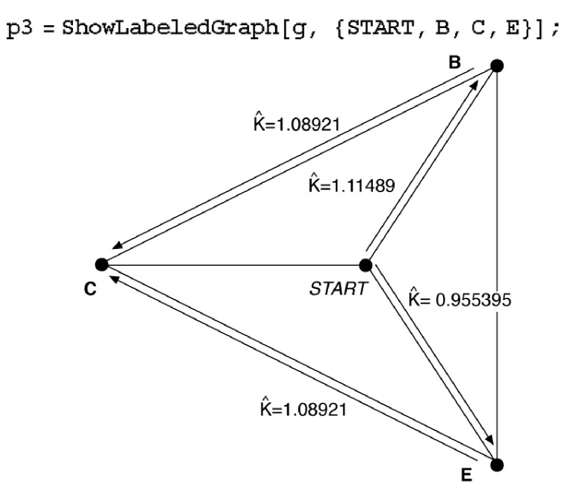
Figure 24: System under Analysis: Components and Topology.

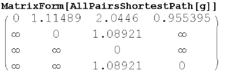
Figure 25: Minimum Complexity Paths Matrix.

In Figure 26 the function CoordVul computes a maximum flow through the K-Map graph using the node positions as shown in Figure 24. Density ($K(x)/l(x)$) from Definition 1, acts as a resistance, while its inverse acts as conductance, supporting insecurity flows as illustrated in Figure 28. The resulting flow matrix in Figure 27 shows the maximum flow through each link. Figure 29 shows the complexity surface of the resulting flows. Higher areas correspond to less vulnerable states, while lower areas correspond to more vulnerable states. Note that in the following contour maps, areas of infinite height are simply shown without a surface. By comparing Figure 24 and Figure 29, it is apparent that the START state, the infinite mountain in the center of the topology, is invulnerable, which makes intuitive sense. State E is the weakest individual component and lowest area on the right side. Note that while State C cannot be directly attacked from the START state, it can be attacked via states B and E, located in the upper and lower right side of the figure respectively, have a relatively intermediate level of vulnerability.

In the insecurity flow contour shown in Figure 30, the density from Definition 1 is resistance and all possible flows from and to every node are summed to obtain an insecurity level. While Node C is assigned infinite complexity as shown in Figure 29, it actually is the most insecure component given that flows exist from Nodes B and E.

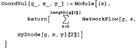
Figure 26: Insecurity Flow Graph.

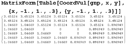
Figure 27: Insecurity Flow Results.

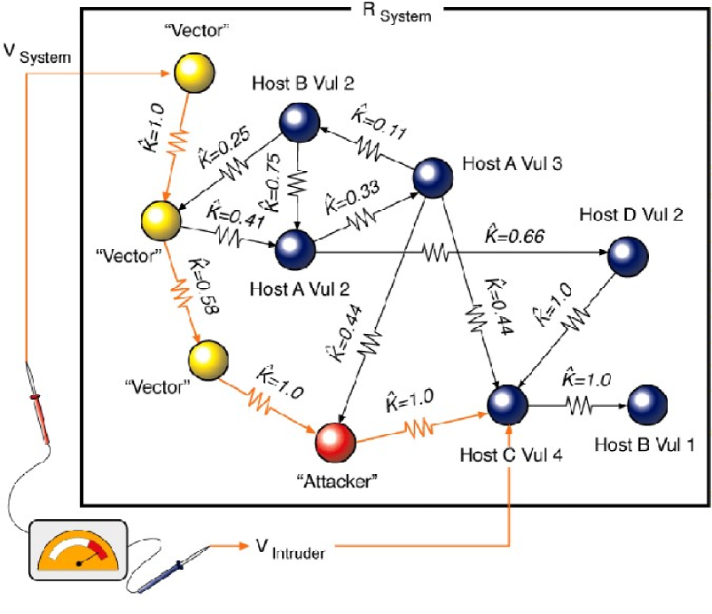
Figure 28: Grid-Based Representation of Information Assurance.

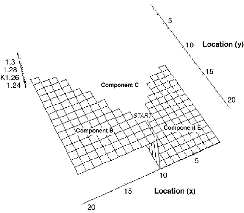
Figure 29: K-Map Contour of System in Figures 24.

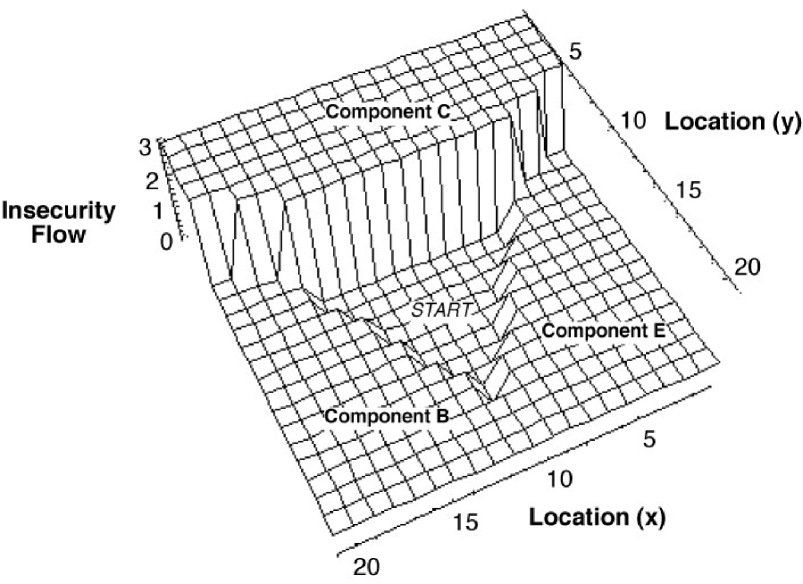
Figure 30: Insecurity Flow Contour of System in Figure 24.

4 . Summary

A Kolmogorov Complexity estimate was used within the Active Virtual Network Management Prediction framework in order to characterize and improve system performance. The application in this paper focused on an active network in which information, algorithmic and static, was transmitted to support prediction for active network management. However, the results are ubiquitously applicable to algorithmic transmission of information in general. Kolmogorov Complexity was experimentally validated as a theory describing the relationship between algorithmic compression, complexity, and prediction accuracy within an active network. Next the relationship between complexity and vulnerability analysis was proposed. Finally, this work sets the stage for research into self-composing solutions based upon Kolmogorov Complexity which will be the focus of the next phase of this project.

4.1 . Acknowledgments

The work discussed in this paper was funded in full by DARPA, under the auspices of the Fault Tolerant Networks program. Our thanks go to Doug Maughan, the Active Networks program manager and Scott Shyne, Air Force Rome Labs for their generous support.

References

- [1] A.-L. Barabasi, V. W. Freeh, H. Jeong, and J. B. Brockman. Parasitic computing. Nature, 412:894–897, Aug. 2001.
- [2] S. F. Bush. Active Virtual Network Management Prediction. In PADS ’99, May 1999.
- [3] S. F. Bush and S. C. Evans. Kolmogorov complexity for information assurance. Technical Report 2001CRD148, General Electric Corporate Research and Development, 2001.
- [4] S. F. Bush and A. B. Kulkarni. Active Networks and Active Network Management: A Proactive Management Framework. Kluwer Academic/Plenum Publishers, ISBN 0-306-46560-4, 2001.
- [5] S. F. Bush, A. B. Kulkarni, V. Galtier, K. Mills, and Y. Carlinet. Prediction and controlling resource usage in a heterogeneous active network, Dec. 2000. DARPA Active Networks PI Meeting and Demonstration (http://www.crd.ge.com/~bushsf/an).
- [6] S. C. Evans and S. F. Bush. Symbol compression ratio for string compression and estimation of kolmogorov complexity. Technical Report 2001CRD159, General Electric Corporate Research and Development, 2001.
- [7] S. C. Evans, S. F. Bush, and J. E. Hershey. Information assurance through kolmogorov complexity. In DARPA Information Survivability Conference and Exposition II (DISCEX-II 2001), volume II, pages 322–331, June 2001.
- [8] V. Galtier, K. Mills, Y. Carlinet, S. Bush, and A. Kulkarni. Predicting resource demand in heterogeneous active networks. In Proceedings of MILCOM 2001, Oct. 2001.
- [9] V. Galtier, K. Mills, Y. Carlinet, S. Bush, and A. Kulkarni. Prediction and controlling resource usage in a heterogeneous active network. In Third Annual International Workshop on Active Middleware Services, San Francisco, CA, Aug. 2001.
- [10] W. Kircher, M. Li, and P. Vitanyi. The Miraculous Universal Distribution. The Mathematical Intelligencer, 1997.
- [11] A. B. Kulkarni and S. F. Bush. Active network management, kolmogorov complexity, and streptichrons. Technical Report 2000CRD107, General Electric Corporate Research and Development, dec 2000.
- [12] A. B. Kulkarni and S. F. Bush. Active network management and kolmogorov complexity. In Proceedings of IEEE OpenArch 2001, Apr. 2001.
- [13] A. B. Kulkarni and S. F. Bush. Detecting distributed denial of service attacks using kolmogorov complexity metrics. Submitted to IEEE Computer Security Foundations Workshop, Feb. 2002.
- [14] M. Li and P. Vitanyi. Introduction to Kolmogorov Complexity and its Applications. Springer-Verlag, Aug. 1993.
- [15] G. Y. Liu and G. Q. M. Jr. A Predictive Mobility Management Algorithm for Wireless Mobile Computing and Communications. In International Conference on Universal Personal Communications (ICUPC), pages 268,272, Nov 1995.
- [16] C. S. Wallace and D. L. Dowe. Minimum message length and Kolmogorov complexity. The Computer Journal, 42(4):270–283, 1999.