The efficient generation of unstructured control volumes in 2D and 3D

Abstract

Many problems in engineering, chemistry and physics require the representation of solutions in complex geometries. In the paper we deal with a problem of unstructured mesh generation for the control volume method. We propose an algorithm which bases on the spheres generation in central points of the control volumes.

1 Introduction

An unstructured mesh generator can solve many of the problems associated with the structured meshes. The unstructured meshes are suitable for complex geometries, especially when we use the control volume method [10]. The control volume method on the one hand, is based upon the simple physical principle of a flux balance. Nevertheless, the generated meshes have to fulfill some restrictions for such method. One of the conditions says than lines connecting the central point in the control volume with neighbour central points have to be perpendicular to the sides of the neighbour volumes. However, the neighbourhood of each neighbour or cell in an unstructured mesh must be defined explicitly. This is one disadvantage of unstructured meshes because it has to reserve large storage of the computer memory. Nevertheless, the advantages like easy for handling adaptability in time, ability to generate meshes about arbitrary geometries. We can divide such meshes into the cell-vertex control volumes and the cell-centered control volumes. In the cell-vertex volumes, all elements containing the relevant point are applied as a control volume, so the control volumes overlap. In the cell-centered control volumes the elements are subdivided and the control volumes do not overlap.

In this paper we propose a generator for unstructured cell-centered volumes, which is useful for the control volume method [10]. The mesh is constructed for a number of points randomly located in a domain and the domain border.

2 Mathematical background

We turn our attention in two and three dimensional space. Let us consider a domain $\Omega\subset R^{3}$ with smooth its boundary $\partial\Omega$. In such domain and boundary we generate randomly a set of points $P_{i}(a,b,c)$, where $i=1..N$. The points establish cell-centers, around of which we determine convex polygons. The polygons are the non-overlapping control volumes which are applied in the control volume method [10]. We can formulate two groups of basic assumptions necessary for the meshes construction as follows:

1. global conditions:

   such domain has to be consistent,

   edges of some polygon have the same lengths to the corresponding edges of neighbour polygons,

2. local conditions:

   inside a polygon one may found only one random point called the cell-center or the point,

   an edge of the polygon has to be perpendicular to the line connecting two points.

If we fulfill the global assumptions, we may discretize the domain $\Omega$ through its division into the triangles in $R^{2}$ space or into the tetrahedrons in $R^{3}$ space. Such discretization is a standard solution, which one may find in convex geometry [4] through Delaunay triangulation [1, 8, 11]. Regarding to the global and local conditions we take into consideration a fact, that we cannot generate polygons in $R^{2}$ which overlap neighbour polygons. The fact also exist for the generated tetrahedrons in $R^{3}$ space.

In this paper we propose a novel algorithm for generation of control volumes. We start the algorithm in two dimensions because one can see how it works. We consider circles with unknown radiuses which centers are located in the points, which are randomly located in the domain $\Omega$. Let us assume, that within the triangle created by the points the circles only in the one point crosses. The point is a vertice of control volumes generated around the point. Following that we need to solve the system of equations

$$(\widehat{x}-a_{l})^{2}+(\widehat{y}-b_{l})^{2}=r_{l}^{2},(l=1,2,3).$$ (1)

Assuming, that the radiuses $r_{l}$ of the circles are unknown, we obtain a point $Q\big{(}\widehat{x}(r_{1},r_{2},r_{3}),\widehat{y}(r_{1},r_{2},r_{3})\big{)}$ which coordinates are solution of the system (1)

$$\left.\begin{array}[]{c}\widehat{x}(r_{1},\,r_{2},\,r_{3})=\frac{-(b_{2}-b_{3})\cdot r_{1}^{2}+(b_{1}-b_{3})\cdot r_{2}^{2}-(b_{1}-b_{2})\cdot r_{3}^{2}+(a_{1}^{2}+b_{1}^{2})\cdot(b_{2}-b_{3})}{2\cdot\left[(a_{1}-a_{2})\cdot(b_{1}-b_{3})-(a_{1}-a_{3})\cdot(b_{1}-b_{2})\right]}+\\ -\frac{(a_{2}^{2}+b_{2}^{2})\cdot(b_{1}-b_{3})+(a_{3}^{2}+b_{3}^{2})\cdot(b_{1}-b_{2})}{2\cdot\left[(a_{1}-a_{2})\cdot(b_{1}-b_{3})-(a_{1}-a_{3})\cdot(b_{1}-b_{2})\right]}\\ \widehat{y}(r_{1},\,r_{2},\,r_{3})=\frac{(a_{2}-a_{3})\cdot r_{1}^{2}-(a_{1}-a_{3})\cdot r_{2}^{2}+(a_{1}-a_{2})\cdot r_{3}^{2}-(a_{1}^{2}+b_{1}^{2})\cdot(a_{2}-a_{3})}{2\cdot\left[(a_{1}-a_{2})\cdot(b_{1}-b_{3})-(a_{1}-a_{3})\cdot(b_{1}-b_{2})\right]}+\\ +\frac{(a_{2}^{2}+b_{2}^{2})\cdot(a_{1}-a_{3})-(a_{3}^{2}+b_{3}^{2})\cdot(a_{1}-a_{2})}{2\cdot\left[(a_{1}-a_{2})\cdot(b_{1}-b_{3})-(a_{1}-a_{3})\cdot(b_{1}-b_{2})\right]}\end{array}\right.$$ (2)

The indexes in formulas (1) and (2) correspond to the local case.

In the global case we have random points $P_{i}(a,b,c),i=1..N$ which are generated inside the domain $\Omega$ and its boundary $\partial\Omega$. We use Delaunay triangulation [1, 8, 11] that to find neighbourhood of point $P_{i}$ defined by several points $P_{j(i,1)}\dots P_{j(i,k)}\dots P_{j(i,M(i))}$. The index $j(i,k)$ is a function which establishes a point number having neighbourhood with the $i$-th point. The temporal index $k$ varies from $1$ to $M(i)$. The $M(i)$ is a number of points corresponding to the $i$-th point. Three points $P_{i},P_{j(i,k)},P_{j(i,k+1)}$ define a triangle. When the temporal index $k+1$ exceeds $M(i)$ then we have $P_{j(i,k+1)}=P_{j(i,1)}$. Moreover, we take into consideration a condition $j(i,k)\neq i$. We extend a definition of formula (2) for the global case putting $(a_{i},b_{i})$, $(a_{j(i,k)},b_{j(i,k)})$, $(a_{j(i,k+1)},b_{j(i,k+1)})$ and $(r_{i},r_{j(i,k)},r_{j(i,k+1)})$ respectively into variables with established indexes. In our approach, we are looking for the radiuses $r_{i}$. Taking into consideration of such fact we formulate a range of radiuses variation as

$$\max\limits_{k}\left[(L_{i,j(i,k)}-r_{max\,j(i,k)})\right]<r_{i}<r_{max\,i},$$ (3)

where $L_{i,j(i,k)}$ is a distance between two neighbour points defined as

$$L_{i,j(i)}=\sqrt{(a_{i}-a_{j(i)})^{2}+(b_{i}-b_{j(i)})^{2}}.$$ (4)

Maximal radius of a circle is formed as

$$r_{max\,i}=\min\limits_{k}\left[h_{i,j(i,k)}\right],$$ (5)

where $h_{i,j(i,k)}$ is a distance defined in acute triangles as

$$\begin{array}[]{c}h_{i,j(i,k)}=\frac{|(b_{j(i,k)}-b_{j(i,k+1)})a_{i}-(a_{j(i,k)}-a_{j(i,k+1)})b_{i}|}{\sqrt{(b_{j(i,k)}-b_{j(i,k+1)})^{2}+(a_{j(i,k)}-a_{j(i,k+1)})^{2}}}+\\ +\frac{|(a_{j(i,k)}-a_{j(i,k+1)})b_{j(i,k+1)}-(b_{j(i,k)}-b_{j(i,k+1)})a_{j(i,k+1)}|}{\sqrt{(b_{j(i,k)}-b_{j(i,k+1)})^{2}+(a_{j(i,k)}-a_{j(i,k+1)})^{2}}}\end{array}.$$ (6)

In acute angles of right and obtuse triangles we have

$$h_{i,j(i,k)}=\min\limits_{k}\left[L_{i,j(i,k)},L_{i,j(i,k+1)}\right].$$ (7)

The symbol $r_{max\,j(i,k)}$ represents a maximal radius of the $j$-th point being a neighbour of the $i$-th point.

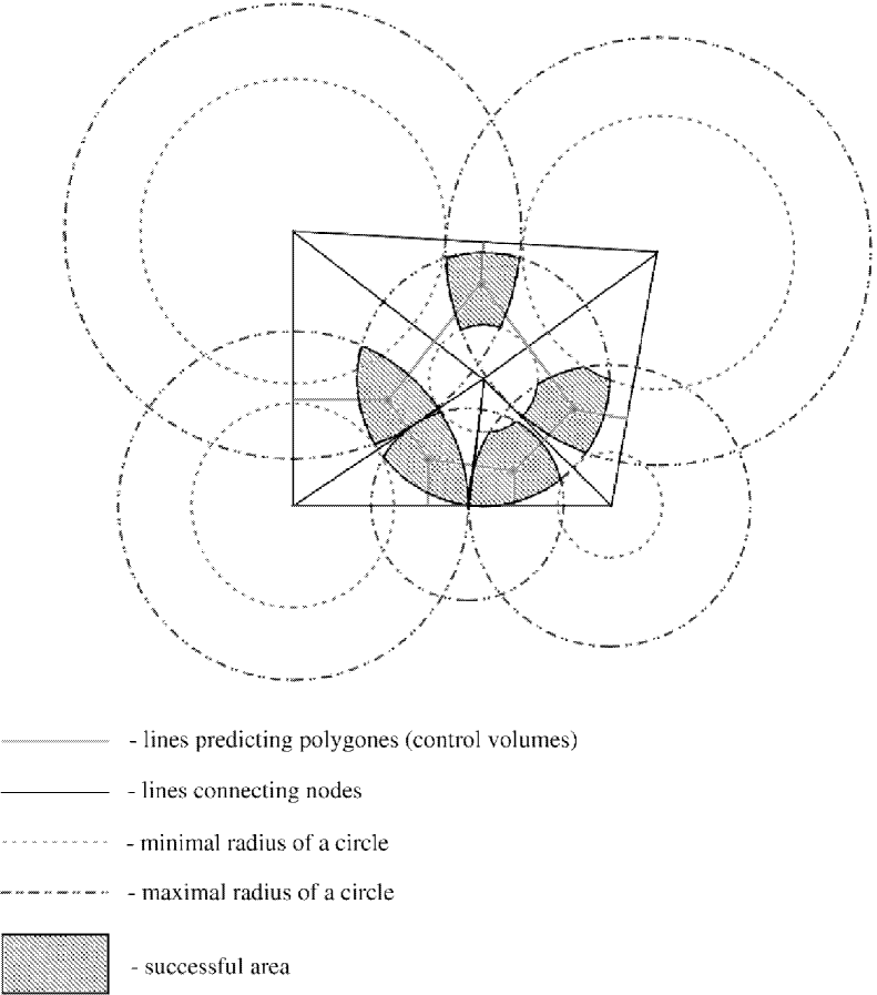
Figure 1: Idea of generation of control volumes.

Using extended formula (2) and additional expressions (3)$\div$(7) one can construct an unstructured mesh. Fig. 1 shows an idea of the control volume generation using the expression (2) and the limit (3). We can observe that the local condition - an edge of the polygon has to be perpendicular to the line connecting two points - is fulfilled. The general algorithm uses some optimisation that to find the points (2) being the vertices of the polygons (control volumes). In this paper we neglect the construction of an objective function because it is not the subject of our consideration. We applied Rosenbrock’s method [6] for the local solution. For the global solution we use the soft selection method [3] which is a global optimisation method. Prediction of the unstructured mesh under such way is not only the one way of the mesh construction. It is possible to construct another type of mesh without restriction that expression (2) is a solution of eqn. (1). But we have to restrict the expression (3) because it guaranties right mesh construction for the control volume method [10]. Let us assume that a radius of the circle overlaps other radiuses of the neighbour circles. Of course we have to restrict the condition (3). Corresponding to previous and present mesh construction we have

$$L_{i,j(i,k)}-\big{(}r_{i}+r_{j(i,k)}\big{)}\leq 0.$$ (8)

Following eqn. (8) the point coordinates given by expression (2) are not the solution of the system (1) but they become the coordinates of the point predicted by lines connecting two points of crossing circles. From the other hand, we can assume that a radius of the circle does not overlap other radiuses of the neighbour circles. In such situation we have

$$L_{i,j(i,k)}-\big{(}r_{i}+r_{j(i,k)}\big{)}>0.$$ (9)

One can say, that conditions (8) and (9) allow us to obtain different forms of unstructured meshes. However, in local solution is possible some combination of expressions (8) and (9) respectively.

Similar to previous results we consider a set of random points $P_{i}(a,b,c)$ in $R^{3}$ space. Analogously to the previous considerations, we use spatial Delaunay triangulation that to find neighbourhood of point $P_{i}$ which is defined by several points $P_{j(i,k,l)}$. The index $j(i,k,l)$ is a function which establishes a point number having neighbourhood with the $i$-th point. The temporal index $k$ describes a number of tetrahedrons having the common $i$-th point. It varies from $1$ to $N(i)$. The next index $l$ varies from $1$ to $3$ and it is a point number corresponding to the $k$-th tetrahedron. The four points $P_{i},P_{j(i,k,1)},P_{j(i,k,2)},P_{j(i,k,3)}$ define a $k$-th tetrahedron. We search radiuses of spheres which centers are located in the points. In each tetrahedron crosses the four radiuses and they create a point which is the vertice of the control volume. Solving the following system

$$(\widehat{x}-a_{l})^{2}+(\widehat{y}-b_{l})^{2}+(\widehat{z}-c_{l})^{2}=r_{l}^{2},(l=1..4),$$ (10)

we can find the local vertices coordinates

$$\widehat{x}(r_{1},\,r_{2},\,r_{3},\,r_{4})=\frac{W_{x}}{W},\hskip 5.69054pt\widehat{y}(r_{1},\,r_{2},\,r_{3},\,r_{4})=\frac{W_{y}}{W},\hskip 5.69054pt\widehat{z}(r_{1},\,r_{2},\,r_{3},\,r_{4})=\frac{W_{z}}{W},$$ (11)

where

$$W=\left|\begin{array}[]{ccc}2(a_{1}-a_{2})&2(b_{1}-b_{2})&2(c_{1}-c_{2})\\ 2(a_{1}-a_{3})&2(b_{1}-b_{3})&2(c_{1}-c_{3})\\ 2(a_{1}-a_{4})&2(b_{1}-b_{4})&2(c_{1}-c_{4})\\ \end{array}\right|,\hskip 8.53581ptW_{x}=\left|\begin{array}[]{ccc}\triangle_{1}&2(b_{1}-b_{2})&2(c_{1}-c_{2})\\ \triangle_{2}&2(b_{1}-b_{3})&2(c_{1}-c_{3})\\ \triangle_{3}&2(b_{1}-b_{4})&2(c_{1}-c_{4})\\ \end{array}\right|,$$

$$W_{y}=\left|\begin{array}[]{ccc}2(a_{1}-a_{2})&\triangle_{1}&2(c_{1}-c_{2})\\ 2(a_{1}-a_{3})&\triangle_{2}&2(c_{1}-c_{3})\\ 2(a_{1}-a_{4})&\triangle_{3}&2(c_{1}-c_{4})\\ \end{array}\right|,\hskip 8.53581ptW_{z}=\left|\begin{array}[]{ccc}2(a_{1}-a_{2})&2(b_{1}-b_{2})&\triangle_{1}\\ 2(a_{1}-a_{3})&2(b_{1}-b_{3})&\triangle_{2}\\ 2(a_{1}-a_{4})&2(b_{1}-b_{4})&\triangle_{3}\\ \end{array}\right|$$

and

$$\triangle_{1}=r_{2}^{2}-r_{1}^{2}+a_{1}^{2}-a_{2}^{2}+b_{1}^{2}-b_{2}^{2}+c_{1}^{2}-c_{2}^{2},$$

$$\triangle_{2}=r_{3}^{2}-r_{1}^{2}+a_{1}^{2}-a_{3}^{2}+b_{1}^{2}-b_{3}^{2}+c_{1}^{2}-c_{3}^{2},$$

$$\triangle_{3}=r_{4}^{2}-r_{1}^{2}+a_{1}^{2}-a_{4}^{2}+b_{1}^{2}-b_{4}^{2}+c_{1}^{2}-c_{4}^{2}.$$

Similar to previous mesh construction, we define lower and upper limits of the radiuses variation

$$\max\limits_{k,l}\left[(h_{i,j(i,k,l)}-r_{max\,j(i,k)})\right]<r_{i}<r_{max\,i}.$$ (14)

The symbol $h_{i,j(i,k,l)}$ represents height of a triangle being the wall of the tetrahedron and for the acute triangles is defined by the following formula

$$\begin{array}[]{c}h_{i,j(i,k,l)}=\sqrt{\frac{\left(BB_{12}\cdot CC_{32}-BB_{32}\cdot CC_{12}\right)^{2}\left(AA_{32}\cdot CC_{12}-AA_{12}\cdot CC_{32}\right)^{2}+}{AA_{32}^{2}+BB_{32}^{2}+CC_{32}^{2}}}+\\ \sqrt{\frac{\left(AA_{12}\cdot BB_{32}-AA_{32}\cdot BB_{12}\right)^{2}}{AA_{32}^{2}+BB_{32}^{2}+CC_{32}^{2}}}\end{array},$$ (15)

where

$$AA_{12} = a_{i}-a_{j(i,k,l)},\hskip 14.22636ptAA_{32}=a_{j(i,k,l+1)}-a_{j(i,k,l)},$$

$$BB_{12} = b_{i}-b_{j(i,k,l)},\hskip 14.22636ptBB_{32}=b_{j(i,k,l+1)}-b_{j(i,k,l)},$$

$$CC_{12} = c_{i}-c_{j(i,k,l)},\hskip 14.22636ptCC_{32}=c_{j(i,k,l+1)}-c_{j(i,k,l)}.$$

In acute angles of right and obtuse spatial triangles we have

$$h_{i,j(i,k,l)}=\min\limits_{l}\left[L_{i,j(i,k,l)},L_{i,j(i,k,l+1)}\right],$$ (16)

where $L_{i,j(i,k,l)}$ is a spatial distance defined between two points as

$$L_{i,j(i,k,l)}=\sqrt{\left(a_{i}-a_{j(i,k,l)}\right)^{2}+\left(b_{i}-b_{j(i,k,l)}\right)^{2}+\left(c_{i}-c_{j(i,k,l)}\right)^{2}}.$$ (17)

When the temporal index $l+1$ exceeds $3$ then we put $P_{j(i,k,l+1)}=P_{j(i,k,1)}$. Maximal radius of a sphere is defined as

$$r_{max\,i}=\min\limits_{k}\left[H_{i,j(i,k)}\right].$$ (18)

However, the function $H_{i,j(i,k)}$ is height of a tetrahedron created by the vertices $P_{i},P_{j(i,k,1)},P_{j(i,k,2)},P_{j(i,k,3)}$ and for the acute tetrahedron we have

$$H_{i,j(i,k)}=\frac{|A\cdot a_{i}+B\cdot b_{i}+C\cdot c_{i}+D|}{\sqrt{A^{2}+B^{2}+C^{2}}}$$ (19)

where

$$A=m_{21}\cdot n_{31}-m_{31}\cdot n_{21}, \hskip 14.22636ptB=d_{31}\cdot n_{21}-d_{21}\cdot n_{31},$$

$$C=d_{21}\cdot m_{31}-d_{31}\cdot m_{21}, \hskip 14.22636ptD=-A\cdot a_{j(i,k,1)}-B\cdot b_{j(i,k,1)}-C\cdot c_{j(i,k,1)}$$

and

$$d_{21}=a_{j(i,k,2)}-a_{j(i,k,1)},\;m_{21}=b_{j(i,k,2)}-b_{j(i,k,1)},\;n_{21}=c_{j(i,k,2)}-c_{j(i,k,1)},$$

$$d_{31}=a_{j(i,k,3)}-a_{j(i,k,1)},\;m_{31}=b_{j(i,k,3)}-b_{j(i,k,1)},\;n_{31}=c_{j(i,k,3)}-c_{j(i,k,1)}.$$

But for the right and obtuse tetrahedrons we have

$$H_{i,j(i,k)}=\min\limits_{l}\left[h_{i,j(i,k,l)}\right].$$ (20)

The symbol $r_{max\,j(i,k)}$ represents a maximal radius of $j$-th point being a neighbour of the $i$-th point.

3 Example of calculations

In practical mesh construction when expression (3) is fulfilled we obtain a unique solution. Fig. 2 shows an example of mesh created under restriction that formula (2) is a solution of the system (1). Fig. 2a presents triangulation of some points in which generated circles. Within the triangle crosses the circles only in one point. According to the previous description we draw control volumes presented by Fig. 2b. Nevertheless, we can construct a mesh without restriction that formula (2) is a solution of the system (1). We can apply conditions (8) or (9) respectively. In this case we generate a mesh much more easier than in previous case. Expressions (8) and (9) extend our considerations for different generation of meshes.

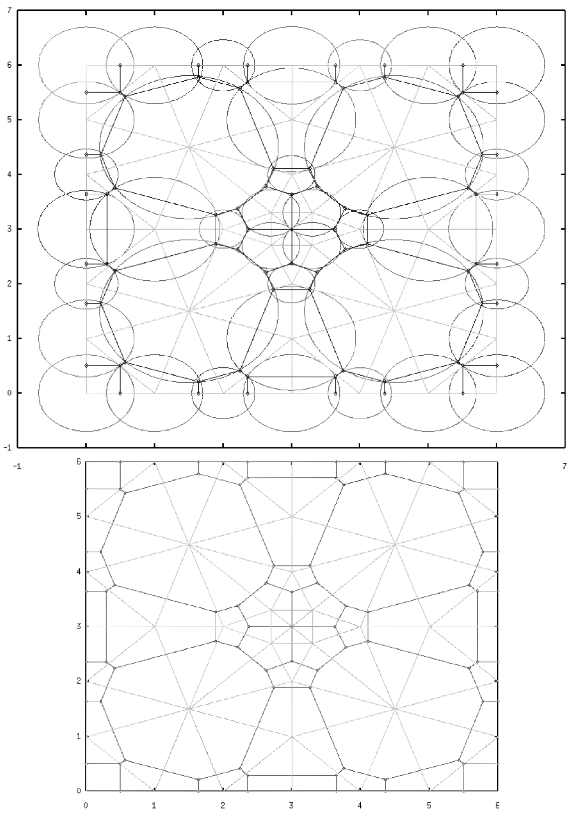
Figure 2: Example of control volumes taking into consideration that formula (2) is a solution of the system (1): a) random points after triangulation; b) forms of control volumes.

4 Concluding remarks

In this paper we elaborate a new method of generation of unstructured meshes. The algorithm is prepared for the control volume method in two- and three dimensional space. For random location of points we use Delaunay triangulation before the mesh generation. Our method bases in 3D on circles generation in the points. Within one triangle created by three points crosses the circles in one point. The point is a vertice of a control volume. We extend our considerations for the triangles in which are overlapping or non-overlapping circles. The extension allow us to generate meshes much more easier than in previous case. In opposite to the Thyssen polygons we can generate control volumes for the right and obtuse triangles. However, our method is suitable and easy to use in generation of control volumes in three dimensional space.

References

- [1] Chiang Y. J., Tamassia R.: Dynamic algorithms in computational geometry, Proc. IEEE 80(9), (1992) 1412-1432
- [2] Elmahi I, Benkhaldoun F.: Finite volume simulation of interval of a droplet flame ignition on unstructured meshes, Journal of Computational an Applied Mathematics, 103, (1999) 187-203
- [3] Galar R.: Soft selection in Random Global Adaptation in . A biocybernetic model of development, Mongraph 17, Wroclaw University of Technology, Wroclaw (Poland), (1990) (in polish)
- [4] Gruber P.M., Wills J.M.: Handbook on Convex Geometry, vol. A, B, North-Holland, (1993)
- [5] Jorgenson P. C. E., Pletcher R. H.: An implicit numerical scheme for the simulation of interval viscous flow on unstructured grids, Computers & Fluids 5, (1996) 447-466
- [6] Kunzi H. P., Tzschach H. G., Zehnder C. A.: Numerical methods of mathematical optimization with Algol and Fortran programmes, Academic Press (1971)
- [7] Neises J., Steinbach I.: Finite element integration for the control volume method, Communications in numerical methods in engineering 12, (1996) 543-555
- [8] Orkisz J.: Finite difference method, in: Kleiber M. (ed.), Computational methods in solid mechanics, PWN, Warsaw (1995) (in polish)
- [9] O’Rourke J.: Computational geometry in C, Cambridge University Press (1995)
- [10] Patankar V. S.: Numerical heat transfer and fluid flow, Hemisphere, New York, (1980)
- [11] Renka R. J., Algorithm 772: STRIPACK: Delaunay triangulation and Voronoi diagram on the surface of a sphere, ACM Trans. Math. Soft. 23(3), (1997) 416-434