[cs/0202028] Classes of service under perfect competition and technological change: a model for the dynamics of the Internet?

1 Introduction

1.1 Background

Consider a delivery service. The quality of the service given may be measured by the delay with which the object is delivered. A service guaranteeing same day delivery is of higher quality than one that guarantees only next day delivery, or delivery within three-business days. Assuming that the service can be provided on a continuous range of qualities, it is typically unrealistic to assume that a service provider could provide all those different services to the customers requiring them or bill them differentially for the qualities requested. In many situations, the service provider will have to decide on certain discrete qualities, i.e., classes of service, and will provide only services of those specific qualities.

The price paid by the different customers depends only on the quality of the service they receive, not on the (inferior) quality they requested and all customers getting the same service pay the same price. We assume that every customer has sharp requirements concerning the quality of service he requests: he will under no circumstances accept a quality that is inferior to his requirements, even if this is much cheaper, and he will, as long as the price is agreeable, use the service of the least quality that is superior or equal to his request. This assumption is not usual, and not in line with [GibbensMasonStein:99] for example. Nevertheless, it is very reasonable in connection with Internet services: there is quite a sharp boundary between delays, jitters and latencies that allow for the streaming of video content and those that do not.

We assume significant economies of scale to the service provider: the cost of providing $w$ services grows less than linearly with $w$ , but we also assume that services of different qualities do not aggregate to generate economies of scale: the cost of providing two classes of service is the sum of the costs of those two different services. This is obviously a severe assumption. In practice, a company offering a few different qualities of service will benefit from economies of scale across those different services: administrative services for example will be shared. But if one considers only the cost of moving packets over the Internet and one assumes, in no way a necessary assumption but a definite possibility (see [Odlyzko:PMPEC99]), that separate sub-networks are affected to the different qualities of service, then the assumption will be satisfied. In the sequel we may therefore assume that a firm provides only a single quality of service: different firms may provide different qualities of service. In deciding what quality or qualities of service to provide, a firm has to avoid two pitfalls: offering a service of poor quality may cater to a share of the market that is too small to be profitable, offering a service of high quality may involve costs that are too high to attract enough customers. A monopoly will set a quality of service and a price that maximize its revenues, but, in a competitive environment, a customer will buy from the provider offering the lowest price for a service whose quality is superior or equal to the quality requested. This will, in general, result in a lower quality of service, a lower price and a higher activity.

Will more than one class of service be proposed? How many? What will the price structure of those classes be? The relation between the traffics in those different classes? Between the revenues gathered in giving those services of different qualities?

Those questions may be asked in many different situations, but they are particularly relevant in connection to the Internet. The Internet delivers packets of information from a source to a destination. The IPv4 protocol, the current protocol for the Internet, reserves three bits in each packet for specifying the quality of service desired, but does not use those bits and treats all packets equally. End users rarely pay per packet and usually pay a flat rate. A number of companies have prepared products for QoS (quality of service), i.e., for controlling an Internet-like network in which packets are treated differentially, but the need for such products is not yet proven. A survey of the different proposals for QoS may be found in [FergHust:98]. Since the Internet is a loose organization that is the product of cooperation between very diverse bodies, billing for such services would also be a major problem. Many networking experts have therefore claimed that the current fat dumb pipe model is best and argued that it will prevail due to the rapid decline in the cost of equipment. A discussion of the different predictions about the evolution of the Internet may be found in [Odlyzko:PMPEC99], where a specific proposal, Paris Metro Pricing (PMP) is advocated. Much interesting information about the economics of the Internet is found at [Varian:website]. An important aspect of the economy of the Internet is that the prices of the networking equipment are dropping very rapidly. One wonders about the consequences of this rapid decline on the price structure.

1.2 Main results

Answers to the questions above are obtained, assuming a one-dimensional ordered continuum of qualities of service, significant economies of scale and a competitive environment. Under some reasonable and quite general assumptions about the demand curve and the cost function, and assuming that a change in price has a similar effect on the demand for all qualities of service, it is shown that one obtains one of two situations.

•

(UC regime) If the demand for services of high-quality is strong and the economies of scale are substantive, then a service provider may satisfy requests for service of arbitrary quality: there will be only one class of service catering for everybody’s needs; this is the fat dumb pipe model.
•

(DC regime) In other cases, a number of classes of service will be proposed and priced according to the quality of the service provided. Very high quality services may not be provided at all.

The DC regime just described may appear in one of two sub-regimes:

•

(BDC regime) A finite number of classes of service are offered and services of very high quality are not offered at all.
•

(UDC regime) An infinite number of classes and all qualities of service are offered.

Notice that, for example, it cannot be the case that a finite number larger than one of classes are offered and that the highest quality of service caters for unbounded qualities. Significant economies of scale and high demand for high-quality services imply a UC regime, independently of the way prices influence demand. When not in a UC regime, high sensitivity of demand to price implies a BDC regime whereas low sensitivity implies an UDC regime. In a BDC regime, when the basic price of the equipment drops, new classes of service will be offered to the high-end customers that could not be profitably catered for previously. In the UC regime, a slowing of the decline in the price of equipment, does not cause the appearance of multiple classes of service. In a DC regime, a change in the price of equipment cannot cause a transition to a UC regime.

A decline in equipment prices, in a DC regime, does not change the boundaries between the different classes of service, but new classes catering to the high-end of the market become available when prices are low enough to make them profitable. The prices drop for all classes, but they drop dramatically for the newly created classes. The ratio of the prices between a class of service and the class just below it decreases and tends to some number typically between $1.5$ and $3$ , depending on the exact shape of the distribution of demand over different qualities and the size of the economies of scale, when prices approach zero. Traffic increases when equipment prices decrease. The direction in which revenues change depends on the circumstances, but, typically, revenues go up and then down when equipment prices decrease. The traffics in neighboring classes of service tend to a fixed ratio when prices approach zero.

2 Previous work

This work took its initial inspiration in the model proposed by A. Odlyzko in the Appendix to [Odlyzko:PMPEC99]. In [Odlyzko:PMPEC99, FishOdly:98], the authors study the case of two different types of customers each type requesting a specific quality of service. They show that, in certain cases, two classes of service will be proposed. The present work assumes a continuous distribution of types of customers. The model of [GibbensMasonStein:99] is more detailed than the one presented here and addresses slightly different questions, but its conclusions are supported by the present work.

The situation described in this paper may seem closely related to the well-studied phenomenon of non-linear pricing [Wilson:Nonlinear]. A second look seems to indicate major differences:

•

here the pricing is linear: a customer given many services pays for each of those separately and, in the end, pays the sum of the prices of the services received,
•

the cost of providing services is assumed to exhibit significant economies of scale, whereas costs are assumed to be additively separable among customers and qualities in most works on non-linear pricing,
•

the present work deals with a competitive environment whereas many works on non-linear pricing assume a monopoly situation.

3 Model and assumptions

The results to be presented are very general, i.e., they hold under very mild hypotheses concerning the form of the cost function and the demand curve, and this is the main reason for our interest in them. Nevertheless, describing exactly the weakest hypotheses needed for the results to hold would lead to a paper loaded with mathematical details distracting the reader from the essentials. Therefore, the conditions under which those general results hold will not be described precisely and those results will be only justified by hand waving. Precise results will deal with two specific parametrized families of functions for cost and demand, described in (2) and (3).

We consider a service that can be given at a continuum of different levels of quality, e.g., the acceptable delay in delivering a packet over the Internet. In this paper, quality is assumed to be one-dimensional (and totally ordered). This is a severe assumption. Quality of service over the Internet is generally considered to be described by a three-dimensional vector: delay, latency and jitter. In this work the quality of service is characterized by a real number $q\geq 1$ . A service quality of $1$ is the lowest quality available. How does a service of quality $q$ compare with a service of quality $1$ ? The following will serve as a quantitative definition of the quality $q$ of a service:

Quality The cost of providing a service of quality $q$ is the cost of providing $q$ services of quality $1$ .

We assume significant economies of scale: the cost of providing $w$ services of quality $1$ grows like $w^{s}$ for some $s$ , $0<s<1$ : the smaller the value of $s$ , the larger the economies of scale. In [FishOdly:98] one may find a discussion of which $s$ best fits the Internet data: values between $1/2$ and $3/4$ seem reasonable. The cost of providing $w$ services of quality $1$ is therefore:

{cost}=c\>{w}^{s}

where $c$ is some positive value that characterizes the price of the equipment. The number $c$ represents the level of the technology, it is a technological constant. Many studies indicate that the price of computer and Internet equipment is decreasing at a rapid pace, probably exponentially. The dynamics of our model is described by a decrease in the value of $c$ .

The cost of providing $f(q)$ services of quality $q$ for every $q$ is:

{cost}=c\>\left(\int_{1}^{\infty}\!q\>f(q)\>dq\right)^{s}.

As is customary, we include the profits in the costs and will describe the equilibrium by an equation equating costs and revenues. Note that the equation above expresses the fact that economies of scale are obtained only among services of the same quality and do not obtain for performing services of two different qualities.

The second half of our model consists of a demand curve describing the demand for services of quality $q$ at price $p$ . We assume that the demand for such services is described by a density function $d(q,p)$ . The demand for services of quality between $a$ and $b>a$ is:

{demand}=\int_{a}^{b}\!d(q,p)\>dq

if the price of any such service is $p$ . Notice that we assume that services of different quality are priced identically. It is very difficult to come up with justifiable assumptions about the form of the demand function $d(q,p)$ . One may assume that, for any fixed $q$ , the value of $d(q,p)$ is decreasing in $p$ , and even approaches zero when $p$ tends to infinity. The rate of this decrease is much less clear. For a fixed $p$ , how should $d(q,p)$ vary with $q$ ? Equivalently, what is the distribution of the demand over different qualities of service? This is not clear at all. Both cases of $d(q,p)$ increasing and decreasing in $q$ will be considered. Fortunately, our results are very general and need not assume much about those questions. There are two assumptions we must make, though. They will be described and discussed now. The first one is that the effect of price on the demand is similar at all quality levels, or that the distribution of demand over $q$ is the same at all prices. We assume that the function $d$ is the product of two functions, one that depends only on $q$ and one that depends only on $p$ . In the absence of information (difficult to obtain) on the exact form of the demand curve, this sounds like a very reasonable first order approximation.

{\bf Decoupling}\ \ d(q,p)=f(q)\>h(p)

(1)

The function $f$ describes the distribution of the demand over different qualities of service. The (decreasing) function $h$ describes the effect of price on the demand. Our results depend on this Decoupling Assumption but should be stable under small deviations from this approximation. The problem of studying systems in which this assumption does not hold is left for future work. Our second assumption is that the function $f$ is constant in time, i.e., does not depend on the technological constant $c$ . Technological progress modifies demand only through price. Our results about the dynamics of the model rely on this assumption.

To be able to prove mathematically precise results, we shall, when needed, assume that:

f(q)=q^{\alpha}

(2)

for some $\alpha$ : the larger the value of $\alpha$ , the larger the relative size of the demand for high-quality services. Is it clear whether $\alpha$ should be positive or negative? Suppose e-mail packets and streaming-video packets can be sent at the same price, would the demand for streaming-video packets be larger than that for e-mail? Probably. It seems that a positive value for $\alpha$ is more realistic, but we do not make any assumption on the sign of $\alpha$ . It may be the case that a more realistic function $f$ should, first, for $q$ ’s close to one, increase, and then decrease for $q$ ’s above the quality required for the most demanding applications at hand. We shall not try to discuss this case here, but the conclusions of this paper offer many qualitative answers even for such a case.

For $h$ , we shall always assume that $h(p)\geq 0$ for every $p\geq 0$ , that $h$ is decreasing when $p$ increases and that, when $p$ approaches $+\infty$ , $h(p)$ approaches zero. Since $h(0)$ characterizes the demand at price $0$ , we shall also assume, for proper scaling, that $h(0)=1$ . The following are examples of possible forms for $h$ :

h(p)=\frac{1}{1+{(a\>p)}^{\beta}},{\rm\ for\ some\ }\beta>0,\ a>0

(3)

In (3), $\beta$ describes the asymptotic rate of decrease of the demand when price increases, but $a$ describes the transient behavior of the demand: the larger $\beta$ , the more sensitive the demand is to price. For $\beta$ close to zero, the demand is little influenced by price, i.e., the demand is incompressible. One may also consider the following:

h(p)=e^{-p},

(4)

h(p)=e^{-p^{2}}.

(5)

As explained at the start of this Section, precise mathematical results will assume that the functions $f$ and $h$ are defined by (2) and (3), but the qualitative results hold for a much larger family of functions.

4 Beginnings

4.1 Equilibrium Equation

As explained in Section 1, we assume that the service provider cannot provide differentiated services: it has to provide the same service and to charge the same price for every service it accepts to perform. Let us, first, assume that there is no service available and that a service provider considers whether or not to enter the market. In a sense, the provider is a monopolist for now. But we shall show below that, because of possible competition, it cannot maximize its profit. It is clear that a provider will choose a quality of service $b$ and a price $p$ , and offer services of quality $b$ at price $p$ to any potential customer. The potential customers are all those customers who request services of quality $q\leq b$ . Customers requesting quality above $b$ will not be served. If there are no competitors, one can hope to attract the totality of the demand for services of quality $q\leq b$ at price $p$ . The size of the demand for service of quality $q$ ( $q\leq b$ ) is $f(q)h(p)$ . Since we provide a service of uniform quality $b$ , the equivalent number of services of quality $1$ that we shall perform is:

\int_{1}^{b}\!b\>f(q)\>h(p)\>dq=b\>h(p)\>A(1,b),

(6)

where we define:

A(a,a^{\prime})=\int_{a}^{a^{\prime}}\!f(q)\>dq.

Note that $A(q,q^{\prime})$ is the demand for services of quality between $q$ and $q^{\prime}$ if the price for those services is zero. The cost of providing the services of (6) is:

{cost}=c\>{b}^{s}\>h^{s}(p)\>A^{s}(1,b).

(7)

The total demand for services is:

{demand}=\int_{1}^{b}\!f(q)\>h(p)\>dq=h(p)\>A(1,b).

(8)

Since every service pays the same price $p$ , the revenue is:

{revenue}=p\>h(p)\>A(1,b).

(9)

Equilibrium is characterized by:

p\>h(p)\>A(1,b)=c\>{b}^{s}\>h^{s}(p)\>A^{s}(1,b),

or equivalently by:

p\>h^{1-s}(p)=c\>{b}^{s}\>A^{-(1-s)}(1,b).

(10)

Equation (10) characterizes the price $p$ as a function of the quality of service $b$ . Most of the remainder of this paper is devoted to the study of this equation.

4.2 Existence of an equilibrium

Given $b$ and $c$ , we want to solve (10) in the variable $p$ . The solutions of (10) are obtained as the intersections of the curve representing the left hand side and a horizontal line representing the right hand side. The left hand side is equal to zero for $p=0$ and is always non-negative. It is reasonable to assume that, considered as a function of $p$ , it has one of the two following forms.

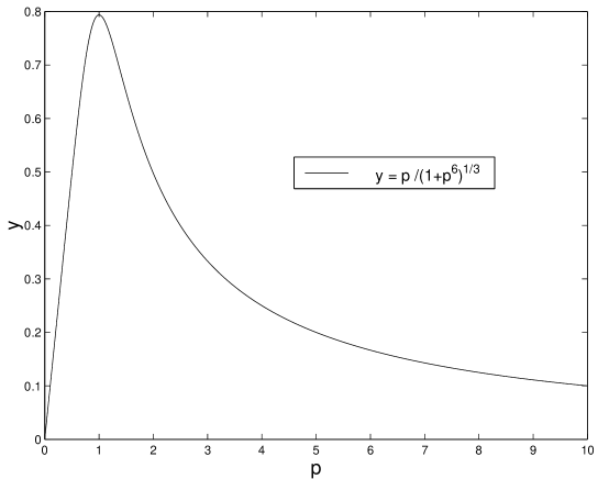
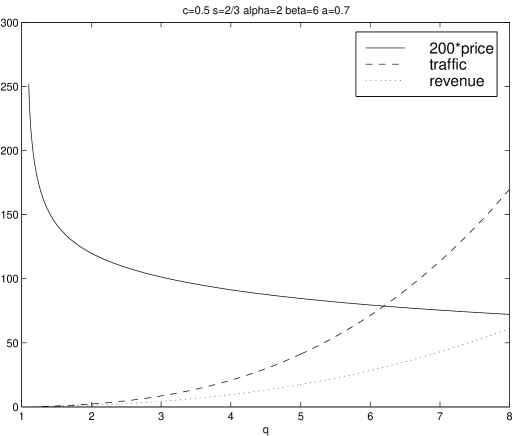
Refer to caption — Figure 1: Left hand side of (10), $s=2/3$ , $\beta=6$

•

Sensitive case: $ph^{1-s}(p)$ increases, has a maximum and then decreases. This seems to be the most typical case: the price has a strong influence on the demand and therefore $h$ is such that $h^{1-s}(p)$ decreases more rapidly than $1/p$ when $p$ is large. This is the case, for any $s$ , when $h$ has the form described in (4) or (5). If $h$ follows (3), it is the case iff $\beta>\frac{1}{1-s}$ . Fig 1 presents a typical sensitive case: $s=2/3$ , $\beta=6$ and $a=1$ , i.e., $h(p)=\frac{1}{1+p^{6}}$ .
•

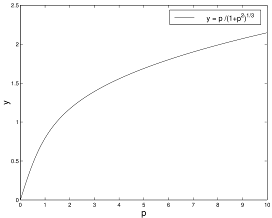
Insensitive case: $ph^{1-s}(p)$ increases always and tends to $+\infty$ when $p$ tends to $+\infty$ . This is the case if the demand is relatively insensitive to the price. It happens if $h$ follows (3) and $\beta<\frac{1}{1-s}$ . The case in which $ph^{1-s}(p)$ increases and approaches a finite value when $p$ tends to $+\infty$ is possible ( $\beta=\frac{1}{1-s}$ ) but not generic. Fig 2 presents a typical insensitive case: $s=2/3$ , $\beta=2$ and $a=1$ , i.e., $h(p)=\frac{1}{1+p^{2}}$ .

Equation (10) behaves quite differently in those two cases. Whereas in the insensitive case, (10) has a unique solution whatever the values of $c$ and $b$ , in the sensitive case we must distinguish between two situations.

•

If the horizontal line is high, e.g., if the technological constant $c$ is large, the horizontal line does not intersect the curve and there is no price $p$ to solve (10). In this case providing a service of quality $b$ is unprofitable, even in the absence of competition and no such service will be provided.
•

If the horizontal line representing the right hand side intersects the curve, for each intersection there is a price $p$ solving (10). In this case, the provider may consider providing a service of quality $b$ at any such price $p$ , but before any more sophisticated analysis, it is clear that the price at which service of quality $b$ will be proposed (if proposed) is the smallest of the $p$ ’s solving (10). If a provider proposes another solution of the equation, a competitor will come in and propose a service of the same quality at a lower price.

In other terms: if (10) has no solution, no service of quality $b$ can be profitably provided, and if (10) has at least a solution then the service may be provided at a price that is the smallest solution of (10).

4.3 Quality of the service provided in a competitive environment

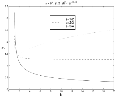
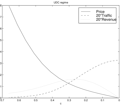
Suppose a service provider finds it is in a situation in which (10) has solutions for some values of $b$ . It may consider providing a service of quality $q$ for any one of those values. The price it will charge, the traffic and the revenue obtained depend on the quality $q$ chosen. To understand the choice that a provider has to make, we need to study (10) in some more depth. Assume that $c$ is given. One would like to know which qualities of service can be profitably provided, i.e., one wants to consider the set of $b$ ’s for which the Equation has a solution. The left hand side of the Equation has been studied in Section 4.2: let us study the right hand side. Under very general circumstances, for $b\rightarrow{1}^{+}$ , $A^{-(1-s)}(1,b)$ approaches $+\infty$ . Figure 3 describes the behavior of the right hand side of (10) as a function of $b$ for different choices of $f$ (i.e. $\alpha$ ) and $s$ . The number $c$ is chosen to be $1$ in all cases. In the leftmost graph $\alpha=1$ and in the rightmost graph $\alpha=-1$ .

The function $b^{s}A^{-(1-s)}(1,b)$ also approaches $+\infty$ for $b$ approaching $1$ and, essentially, it may present any one of two possible behaviors: either it decreases always, or it decreases until it gets to a minimum and then increases without bounds. The case it decreases to a minimum and then increases and approaches a finite value when $b$ tends to $+\infty$ is possible but not generic. These two possible behaviors for the function ${b}^{s}\>A^{-(1-s)}(1,b)$ determine two very different regimes.

Definition 1

In the first regime, the Universal Class regime (UC regime), the right hand side of (10) is a decreasing function of $b$ . In this regime the set of $b$ ’s for which (10) has a solution is an interval of the form $[q_{1},+\infty[$ , for some $q_{1}>1$ . Any service of quality at least $q_{1}$ may be profitably provided. In the second regime, the Differentiated Classes regime (DC regime), the right hand side of (10) decreases, reaches a minimum and increases. One must then distinguish between the sensitive and the insensitive cases. In the sensitive case, the set of $b$ ’s for which (10) has a solution is either empty or an interval of the form $[q_{1},q_{2}]$ , for some $q_{2}\geq q_{1}>1$ . This regime (DC, sensitive case) will be called the BDC (bounded DC) sub-regime. In the insensitive case, (10) has a solution for any $b$ in the interval $[1,+\infty[$ . This regime (DC, insensitive case) will be called the UDC (unbounded DC) sub-regime.

Suppose a service provider finds it is in a situation in which (10) has solutions for some interval of qualities. We know it should choose a quality $q$ in this interval, offer a service of quality $q$ and propose this service at the price $p$ that is the smallest solution to (10). Which $q$ should our provider choose? To each choice for $q$ corresponds a price $p_{q}$ . The number of services performed is given by

{demand}=h(p_{q})\>A(1,q).

Since every service performed is a service of quality $q$ , and every such service is equivalent to $q$ services of quality $1$ , the weighted traffic is:

{traffic}=q\>h(p_{q})\>A(1,q).

The revenue is:

{revenue}=p_{q}\>h(p_{q})\>A(1,q).

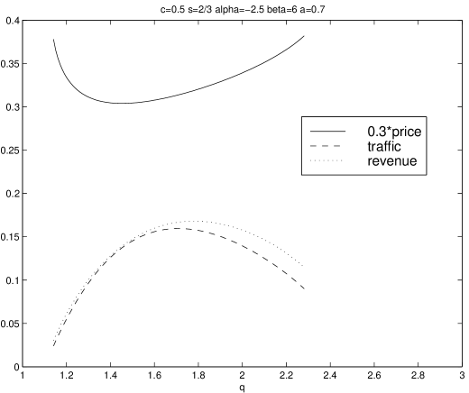
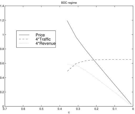
Consider, first, a case typical of the DC regime. In Figure 4 the price $p_{q}$ , the traffic and the revenue are described as functions of the quality $q$ of the service chosen by the provider. The service can be provided only for a bounded interval of qualities. Notice that, in this interval, the price decreases rapidly and then increases slowly, that traffic and revenue increase and then decrease, and that the minimum price is obtained for a quality inferior to the quality that maximizes the revenue.

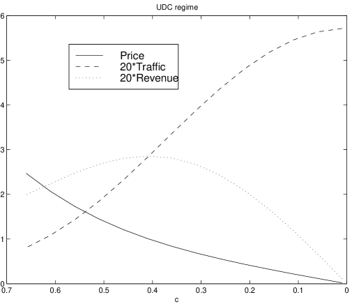
A case typical of the UC regime is described in Figure 5. By our discussion of (10), it is clear that $p_{q}$ is a decreasing function of $q$ . Notice that traffic and revenue increase with $q$ .

What is the quality of service most profitable? Since the revenue includes the profits, one may assume, at first sight, that the first provider to propose such a service will choose the quality $q$ that maximizes its revenue. This analysis is clearly incorrect in a competitive situation. If a provider decides to offer the service that maximizes its revenue, a competitor provider may come in and offer a service of lower quality at a lower price and steal the demand for the lower quality services. Therefore, the price at which the service will be offered is the minimum price possible: the minimum of the function $p_{q}$ on its interval of definition.

Claim 1

The quality $q$ of the service provided is the $q$ for which $p_{q}$ is minimal.

This remark turns out to be of fundamental importance because this quality $q$ , contrary to the quality that maximizes revenue, does not depend on the technological constant $c$ or on the function $h$ that describes the dependence of the demand on the price charged. It depends only on the function $f$ that describes the distribution of the demand over the different qualities of service and on the size of the economies of scale described by the number $s$ . Indeed, this quality $q$ is the value of $b$ that minimizes $b^{s}A^{-(1-s)}(1,b)$ in the DC regime and it is $+\infty$ in the UC regime. There is, therefore, a sharp distinction between the two regimes: in the DC regime a service of finite quality is provided, whereas, in the UC regime, the quality of service provided is high enough to please every customer, i.e., unbounded.

Law 1 (First Law)

Whether or not some service is provided does not depend on the function $h$ that describes the way demand depends on price. It depends on the technological constant $c$ , the size of the economies of scale $s$ , and on the function $f$ that describes the distribution of demand over different qualities of service. If some service is provided its quality depends only on $s$ and $f$ , it does not depend on $c$ or $h$ . In the UC regime, a single class serves requests for services of arbitrary quality and it is given for free. In the DC regime, the service of lowest quality has a finite quality and does not cater for high-end customers. The prevailing regime depends on the form of the economies of scale and on the form of the distribution of the demand over different qualities, it does not depend on the price of the equipment or on the way prices influence demand.

In Section 5, we shall, first, mark the boundary between these two regimes. Then, both regimes: UC and DC will be studied in turn.

5 Between the two regimes

In this Section, we shall assume that $f$ has the form described in (2), for some $\alpha$ , and study the exact boundaries of the UC and DC regimes. The regime is determined by the behavior of the function:

w(b)=b^{s}\>\left(\int_{1}^{b}\frac{dq}{q^{\alpha}}\right)^{-(1-s)},

for $b\geq 1$ . If $w(b)$ has a minimum, then the regime is DC, if it always decreases, the regime is UC. Three cases must be distinguished.

{\rm If\ }\alpha<-1,\ \ w(b)=\frac{b^{s}}{{\left(-\alpha-1\right)}^{-(1-s)}}\;{\left(1-b^{\alpha+1}\right)}^{-(1-s)}.

{\rm If\ }\alpha=-1,\ \ w(b)=b^{s}\>\ln^{-(1-s)}b,

and

{\rm if\ }\alpha>-1,\ \ w(b)=\frac{b^{s}}{{\left(\alpha+1\right)}^{-(1-s)}}\;{\left(b^{\alpha+1}-1\right)}^{-(1-s)}.

For $\alpha<-1$ , we have:

w^{\prime}(b)=\frac{b^{-(1-s)}\>{\left(1-b^{\alpha+1}\right)}^{-(2-s)}}{{\left(-\alpha-1\right)}^{-(1-s)}}\;\left[s(1-b^{\alpha+1})-(1-s)b(-\alpha-1)b^{\alpha}\right],

w^{\prime}(b)=\frac{b^{-(1-s)}\>{\left(1-b^{\alpha+1}\right)}^{-(2-s)}}{{\left(-\alpha-1\right)}^{-(1-s)}}\;\left[(-(2+\alpha)s+\alpha+1)\>b^{\alpha+1}+s\right],

which approaches $s$ and is therefore positive for large $b$ ’s. We conclude that for any $\alpha<-1$ the regime is DC.

For $\alpha=-1$ ,

w^{\prime}(b)=b^{s-1}\>\ln^{-(2-s)}b\>\left[s\ln b-(1-s)\right],

which is also positive for large $b$ ’s. For $\alpha=-1$ the regime is DC.

For $\alpha>-1$ , we have:

w^{\prime}(b)=\frac{b^{-(1-s)}\>{\left(b^{\alpha+1}-1\right)}^{-(2-s)}}{{\left(\alpha+1\right)}^{-(1-s)}}\;\left[s(b^{\alpha+1}-1)-(1-s)b(\alpha+1)b^{\alpha}\right]

w^{\prime}(b)=\frac{b^{-(1-s)}\>{\left(b^{\alpha+1}-1\right)}^{-(2-s)}}{{\left(\alpha+1\right)}^{-(1-s)}}\;\left[((2+\alpha)s-\alpha-1)\>b^{\alpha+1}-s\right]

For large $b$ ’s, $w^{\prime}(b)$ has the sign of $(2+\alpha)s-\alpha-1$ . We may now conclude our study.

Claim 2

{\rm the\ regime\ is\ DC\ iff\ }\alpha\leq-1{\rm\ or\ }s>\frac{\alpha+1}{\alpha+2},

{\rm the\ regime\ is\ UC\ iff\ }\alpha>-1{\rm\ and\ }s\leq\frac{\alpha+1}{\alpha+2},

The boundary between the two regimes can be seen in Figure 6.

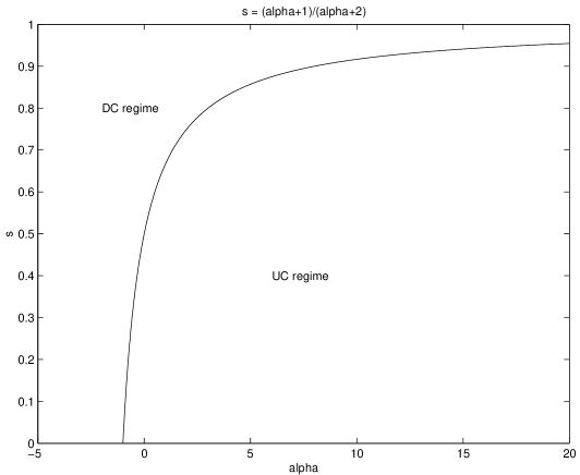
Informally, if the economies of scale are very substantial (small $s$ ) and if high quality services are in big demand ( $f$ grows rapidly), the UC regime prevails. Otherwise, there is an upper bound to the quality of profitable services. There is no profitable way to provide for a service of arbitrary quality because its cost would deter too many potential customers.

6 The universal class regime

6.1 A paradoxical regime

Let us study the UC regime. As discussed in Section 4.3, Figure 5 and in our first Law, in this regime, the right hand side of (10) is as close to zero as one wishes if one takes $b$ to be large enough. For any value of the technological constant $c$ , even a very high one, it is profitable to provide a service of infinite quality at zero price, and therefore, for any value of the technological constant $c$ , a unique class of service of unbounded quality is offered for free. This seems quite a paradoxical situation. The demand (8) and the cost of providing the service (7) are both infinite. The consideration of the revenue is interesting. The revenue (see (9) and (10)) is infinite, but depends linearly on the technological constant $c$ . The revenue drops linearly with the price of the equipment.

This regime seems to fit the fat dumb pipe model of the Internet: there are enough resources to give every request a treatment of the highest quality, there is no need to give differentiated services and the price is very low since the demand is very high and the economies of scale very substantive.

The dynamics of the UC regime under technological progress, i.e., a drop in the constant $c$ , is quite paradoxical. Such a drop does not significantly affect the, already negligible, price of the service, but it affects adversely the (infinite) revenues of the provider.

The First Law implies that the boundary between the UC and DC regimes does not depend on the technological constant $c$ , therefore the answer to the question whether the fat dumb pipe model prevails or whether a number of classes of service will develop depends only on the relation between the economies of scale and the distribution of demand over different qualities, it does not depend on the price of the equipment. Both regimes are stable under technological progress.

6.2 A more realistic model

The paradoxical aspects of the UC regime as described above stem from the consideration of a demand curve that assumes significant demand for services of unbounded quality. It seems more realistic to assume an upper bound to the quality requested from services. A specific example will be given now, to explain what the UC regime may look like in practice. Assume that there is an upper bound $q_{m}$ to the quality of service requested and that the distribution of demand $f$ over different qualities is described by:

f(q)=\left\{\begin{array}[]{ll}q&\mbox{if $1\leq q\leq q_{m}$}\\ 0&\mbox{if $q_{m}\leq q$}\end{array}\right.

(11)

Assume also that $s=\frac{2}{3}$ and that $h(p)=\frac{1}{1+p^{3}}$ . It follows from our discussion above that the service provided, if provided, will be of quality $q_{m}$ . Therefore the equilibrium equation is:

\frac{p}{(1+p^{3})^{1/3}}=2^{1/3}\>c\>{q_{m}}^{2/3}\>{\left({q_{m}}^{2}-1\right)}^{-1/3}.

(12)

The left hand side of (12) has a maximum value of $1$ . For any $c$ such that

c\geq 2^{-1/3}\>{q_{m}}^{-2/3}\>{\left({q_{m}}^{2}-1\right)}^{1/3}

there is no profitable service. For any $c$ smaller than this value, a provider will choose to provide a service of quality $q_{m}$ . The price, traffic and revenue are functions of $c$ and described in Figure 7.

As soon as some service is provided, it caters for all needs. A unique class of service will still prevail in the presence of a drop in the price of equipment, i.e., a decrease in $c$ . Notice that the revenue decreases when the technology constant drops.

7 The differentiated classes regime

Let us study the DC regime now. The best approach is to take a dynamic perspective and consider the evolution of the system under a decrease in the technological constant $c$ .

7.1 The BDC sub-regime

In the first part of this discussion we study the BDC sub-regime, i.e., the sensitive case described in Section 4.2 in which the left hand side of (10) increases to a maximum and then decreases. We have seen that for high $c$ ’s no service is provided. When $c$ falls below a certain value, $c_{0}$ , a service of some finite quality $q_{0}$ is provided. From the First Law we know that, even in the face of further declines in $c$ , the quality $q_{0}$ of the service provided will not change. Two main questions arise:

•

how do the price, the traffic and the revenue of the provider of a service of quality $q_{0}$ evolve under a further decrease in $c$ ?
•

will services of higher quality be offered? which? when? at what price?

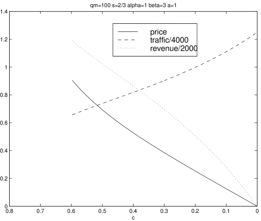
The first question is relatively easily disposed of. Since the right hand side of (10) is a linear function of $c$ , the assumption that the left hand side increases to a maximum implies that the price drops rapidly at first (for $c$ close to $c_{0}$ ), and then at a slower pace. For the functions $h$ considered, the slope of the left hand side is one at $p=0$ and the price $p$ drops essentially linearly with $c$ and approaches zero when $c$ approaches zero. The demand (or the traffic) varies as $h(p)$ and therefore increases very rapidly at first and then approaches some finite value. The revenue varies as $ph(p)$ or $ch(p)^{s}$ . Typically it may exhibit, first, an increase, for values of $c$ at which a drop in the price of the service is over-compensated by an increase in demand and then a decrease. For small $c$ ’s, the revenue drops linearly with $c$ . Figure 8 describes the evolution of price, traffic and revenue for the lowest class of service, the first to be offered on the market.

The second question is deeper. Since a service of quality $q_{0}$ will be provided at a price we have just studied, it is clear that the only customers who could be interested in another service are those requesting a service of quality superior to $q_{0}$ . Will such a service, of quality $b\geq q_{0}$ be provided? The equilibrium equation now becomes:

p\>{h(p)}^{1-s}=c\>{b}^{s}\>A(q_{0},b)^{-(1-s)}.

(13)

Notice that (13) is very similar to (10). A service of quality $b$ may be profitably offered iff (13) has a solution. See Section 4.2 for a discussion: the situation is the same. There is a value $c_{1}$ above which there is no solution and below which there is a solution. Since we are in the sensitive case, the left hand side has a maximum and the price of the service, of quality $b$ , if provided, will be the smallest $p$ satisfying (13).

The discussion of which service will be provided is similar to the discussion found in Section 4.3. The behavior of the right hand side of (13) as a function of $b$ is the same as that of (10). We have assumed we are in the DC regime, and therefore there is a finite value $q_{1}$ for $b$ that minimizes ${b}^{s}\>A(q_{0},b)^{-(1-s)}$ . The service provided will be of a quality $q_{1}$ .

In the case $f$ has the form described in (2), the computation of $q_{1}$ is simplified by a change of variable $q=q_{0}\>q^{\prime}$ .

A(q_{0},b)=\int_{q_{0}}^{b}\!f(q)\>dq=\int_{1}^{b/q_{0}}\!f(q_{0}q^{\prime})\>q_{0}\>dq^{\prime}=q_{0}^{\alpha+1}A(1,b/q_{0})

and the equation becomes:

p\>{h(p)}^{1-s}=c^{\prime}\>{(b/q_{0})}^{s}\>A(1,b/q_{0})^{-(1-s)},{\rm\ for\ }c^{\prime}=c\>q_{0}^{-(\alpha+1)(1-s)+s}.

Notice that

-(\alpha+1)(1-s)+s=(\alpha+2)s-(\alpha+1)>0

by Claim 2 since we are in the DC regime and therefore $c^{\prime}>c$ . Equation (13) is the same as (10), for a larger technological constant, after our change of variable. This implies that the service provided will be of quality $q_{1}$ with

q_{1}/q_{0}=q_{0},{\rm\ i.e.,\ }q_{1}=q_{0}^{2}.

It will appear when

c^{\prime}=c_{0},{\rm\ i.e.,\ }c_{1}=c_{0}\>q_{0}^{(\alpha+1)(1-s)-s}.

The general dynamic picture is now clear. Different classes of service appear as the technological constant $c$ decreases. The $n$ ’th class ( $n\geq 0$ ) appears when $c=c_{0}\>q_{0}^{n(-s+(\alpha+1)(1-s))}$ and it is of quality ${q_{0}}^{n}$ . For any $c>0$ , only a finite number of qualities of service are proposed and no service is provided for request of high quality service. Since, from Section 5, we may also easily compute $q_{0}$ and see that:

{\rm if\ }\alpha<-1,\ \ \ \ q_{0}=\left(\frac{s}{(2+\alpha)s-\alpha-1}\right)^{\frac{1}{\alpha+1}},

{\rm if\ }\alpha=-1,\ \ \ \ q_{0}={e}^{(1-s)/s},

{\rm if\ }\alpha>-1,\ \ \ \ q_{0}=\left(\frac{s}{(2+\alpha)s-\alpha-1}\right)^{\frac{1}{\alpha+1}},

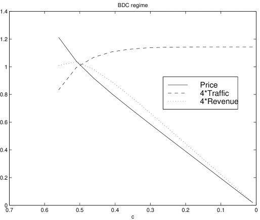
the picture is complete. Figure 9 describes the price, traffic and revenue in the second class of service as functions of the technological constant $c$ , for the same constants as in Figure 8. Compare with Figure 8 and see that the qualitative evolution is similar in both classes.

The ratio of prices in two neighboring classes is interesting to study. The ratio between the prices of service in a class and the class just below, as a function of $c$ , has the same behavior and the same values (for different $c$ ’s) for all classes. Let the classes of services are described by qualities: $q_{0}<q_{1}<\ldots<q_{i}<\ldots$ and appearing for the values of $c$ : $c_{0}>c_{1}>\ldots>c_{i}>\ldots$ . Let $p_{0}(c)<p_{1}(c)<\ldots<p_{i}(c)<\ldots$ be the prices of the corresponding services. The behavior of $p_{1}(c)/p_{0}(c)$ for $c$ between $c_{0}$ and $c_{1}$ is the same as the behavior of $p_{2}(c)/p_{1}(c)$ for $c$ between $c_{1}$ and $c_{2}$ . The price of a newly created class (of high quality) drops (with $c$ ) more rapidly than that of an older class of lower quality and therefore the ratio $p_{i+1}(c)/p_{i}(c)$ , larger than $1$ , decreases with $c$ . Under the assumptions above, it approaches

\left(\frac{s}{(2+\alpha)\>s-\alpha-1}\right)^{\frac{(2+\alpha)\>s-\alpha-1}{\alpha+1}}

when $c$ approaches zero. For $\alpha=-2$ and $s=1/2$ , this gives a value of $2$ , the ratio used by the Paris Metro system when it offered two classes of service, and quite typical of other transportation systems.

7.2 The UDC sub-regime

We may now understand what happens in the insensitive case: the left hand side of (10) grows without bound. In this case, for any $c$ , an infinite number of qualities: $q_{0},q_{1},\ldots,q_{i},\ldots$ of service is offered. The qualities offered are constant, they do not depend on $c$ . Figures 10 and 11 show the first two classes for a generic case.

7.3 The general picture

Law 2 (Second Law)

Under a decrease in the technological constant $c$ , i.e., under technological progress and a drop in the price of equipment:

•

In the UC regime, at any time, i.e., for any value of $c$ , a unique class serves requests for arbitrary quality.
•
In the DC regime,
- –
  
  in the BDC sub-regime, no service is provided at first, then a service of finite quality is provided, later on another service of higher quality will be proposed, and so on. For any quality $q$ a service of quality $q$ will be proposed at some time (and on), but at any time there are qualities of services that are not provided.
- –
  
  in the UDC sub-regime, at any time, an infinite number of classes of service are proposed and requests for arbitrary quality are taken care of.

This Second Law contradicts the folk wisdom that says that the Fat Dumb Pipe (FDP) model for the Internet will collapse when prices become low enough to enable very high quality services. It says that if the FDP model is the one that prevails when $c$ is high, it will continue to prevail after a decrease in $c$ . A drop in the price of equipment cannot cause the breakdown of a system based on a universal class of service.

8 Further work and conclusions

The most intriguing challenges are a theoretical one and an experimental one. The first one concerns the study of the case in which the Decoupling of Equation 1 does not hold, or holds only approximately. The second one is the study of real systems, in particular the Internet, and the evaluation of the parameters of interest for them.

The main conclusion of this work is that the parameters that determine the type of the prevailing market are the size of the economies of scale and the distribution of demand over the range of qualities. The sensitivity of demand to price and the changes in the price of equipment bear a lesser influence.

This paper made two severe assumptions. It assumes perfect competition, and it assumes that economies of scale do not aggregate over different qualities of service. Further work should relax those assumptions.

Classes of service under perfect competition and technological change: a model for the dynamics of the Internet?

Abstract