The Mysterious Optimality of Naive Bayes:
Oleg Kupervasser
Department of Chemical Physics,The Weizmann
Institute of Science,Rehovot 76100, Israel
Abstract
Bayes Classifiers are widely used currently for recognition, identification and knowledge discovery. The fields of application are, for example, image processing, medicine, chemistry (QSAR). However, by mysterious way the Naive Bayes Classifier usually gives a very nice and good presentation of recognition. More complex models of Bayes Classifier cannot improve it considerably. We demonstrate here a very nice and simple proof of the Na ve Bayes Classifier optimality that can explain this interesting fact. The derivation in the current paper is based on
paper of the auther written in 2002.
pacs: PACS numbers 47.27.Gs, 47.27.Jv, 05.40.+j
I Introduction
The derivation in the current paper is based onpaper of the auther written in 2002 KUPER953 Kuper11 Kuper12
Let us give some example from practices of author. The first example was recognition of digits written by hand. Every such digit can be characterized by set of variables. The second example is defect on computer screen scratches, air bubbles, cavities, spots. They can be characterized by set of variables, for example, square of circumscribed ellipse, its eccentricity and so on. The third example is medical diagnostics. We must recognize the diseases on basis of medical symptoms. The all three examples had the same property: in spite of the fact that correlations exist between characteristic variables, the Naive Bayes model gave the excellent result. Moreover, this result could not be improved considerably by using more complex model with some correlations between characteristic variables. Sometimes these correlations (if they are found with errors) can make the model even worse.
In the paper Kuper12 KUPER953 Kuper13 Kuper14 KUPER953
Let us formulate shortly the basic problem that we try to solve in the paper. Suppose that we have a set of some objects and a set of variables that characterize these objects. For every object, we know probability distribution for every variable. However, we have no information about correlations of the variables. Now, suppose that we know variables values for some sample of the objects. What is probability that this sample correspond to some object? It is a typical problem of recognition over a condition of incomplete information.
Let us consider the simplest case when no correlations exist between variables. In this case, the Naive Bayes model is an exact solution of the problem. We prove in this paper that for the case that we know nothing about correlation the Naive Bayes model is not exact, but o p t i m a l 𝑜 𝑝 𝑡 𝑖 𝑚 𝑎 𝑙 optimal
The paper is organized as following. In section II we give exact mathematical definition of the problem for two variables and two objects. In section III we define our notations. In section IV we give generic form of conditional probability for all possible correlations of our variables. In section V we define the restrictions of the functions describing the correlations. In section VI we give the definition a distance between two probability(correlation) models. In section VII we find restrains for our basic functions. In the section VIII we solve our main problem we prove optimality of the Naive Bayes model for uniform distribution of all possible correlations. In the section IX we find mean error between the Naive Bayes model and an actual model for uniform distribution of all possible correlations. In section X we consider the case more than two variables and objects. The last section is conclusions.
II Statement of the problem.
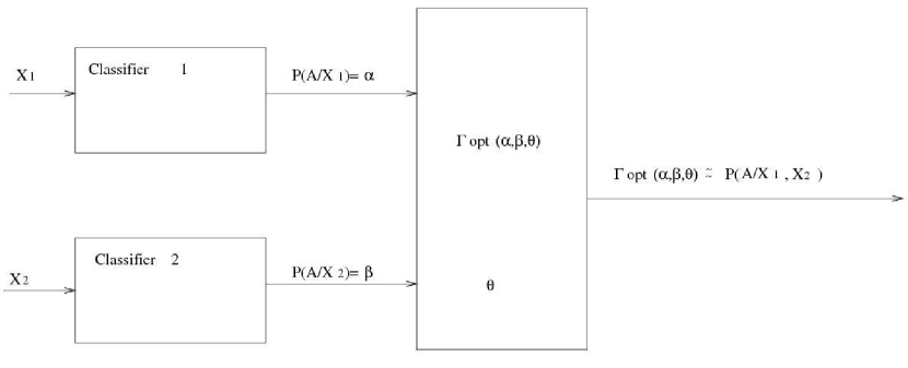
Let A be a random variable, with values in set 0 , 1 0 1
{0,1} a p r i o r i 𝑎 𝑝 𝑟 𝑖 𝑜 𝑟 𝑖 apriori P ( A ) = P ( A = 1 ) 𝑃 𝐴 𝑃 𝐴 1 P(A)=P(A=1) θ 𝜃 \theta X 1 , X 2 subscript 𝑋 1 subscript 𝑋 2
X_{1},X_{2} ] − ∞ ; + ∞ [ ]-\infty;+\infty[ X 1 = x 1 subscript 𝑋 1 subscript 𝑥 1 X_{1}=x_{1} X 2 = x 2 subscript 𝑋 2 subscript 𝑥 2 X_{2}=x_{2} x 1 subscript 𝑥 1 x_{1} x 2 subscript 𝑥 2 x_{2}
P ( A = 1 / X 1 = x 1 ) = P ( A / x 1 ) ≐ α 𝑃 𝐴 1 subscript 𝑋 1 subscript 𝑥 1 𝑃 𝐴 subscript 𝑥 1 approaches-limit 𝛼 P(A=1/X_{1}=x_{1})=P(A/x_{1})\doteq\alpha (1)
P ( A = 1 / X 2 = x 2 ) = P ( A / x 2 ) ≐ β 𝑃 𝐴 1 subscript 𝑋 2 subscript 𝑥 2 𝑃 𝐴 subscript 𝑥 2 approaches-limit 𝛽 P(A=1/X_{2}=x_{2})=P(A/x_{2})\doteq\beta (2)
We wish to estimate the probability P ( A = 1 / X 1 = x 1 , X 2 = x 2 ) = P ( A / x 1 , x 2 ) P(A=1/X_{1}=x_{1},X_{2}=x_{2})=P(A/x_{1},x_{2}) α , β 𝛼 𝛽
\alpha,\beta θ 𝜃 \theta Γ o p t ( α , β , θ ) subscript Γ 𝑜 𝑝 𝑡 𝛼 𝛽 𝜃 \Gamma_{opt}(\alpha,\beta,\theta) P ( A / x 1 , x 2 ) 𝑃 𝐴 subscript 𝑥 1 subscript 𝑥 2 P(A/x_{1},x_{2}) 1
III Notation and preliminaries
ρ X 1 , X 2 ( x 1 , x 2 ) subscript 𝜌 subscript 𝑋 1 subscript 𝑋 2
subscript 𝑥 1 subscript 𝑥 2 \rho_{X_{1},X_{2}}(x_{1},x_{2}) X 1 subscript 𝑋 1 X_{1} X 2 subscript 𝑋 2 X_{2} ρ X 1 , X 2 / A ( x 1 , x 2 ) ≐ h ( x 1 , x 2 ) approaches-limit subscript 𝜌 subscript 𝑋 1 subscript 𝑋 2 𝐴
subscript 𝑥 1 subscript 𝑥 2 ℎ subscript 𝑥 1 subscript 𝑥 2 \rho_{X_{1},X_{2}/A}(x_{1},x_{2})\doteq h(x_{1},x_{2}) X 1 subscript 𝑋 1 X_{1} X 2 subscript 𝑋 2 X_{2} A = 1 𝐴 1 A=1 h ( x 1 , x 2 ) ℎ subscript 𝑥 1 subscript 𝑥 2 h(x_{1},x_{2}) θ 𝜃 \theta P ( A / x 1 , x 2 ) 𝑃 𝐴 subscript 𝑥 1 subscript 𝑥 2 P(A/x_{1},x_{2})
P ( A / x 1 , x 2 ) = θ h ( x 1 , x 2 ) θ h ( x 1 , x 2 ) + ( 1 − θ ) h ¯ ( x 1 , x 2 ) 𝑃 𝐴 subscript 𝑥 1 subscript 𝑥 2 𝜃 ℎ subscript 𝑥 1 subscript 𝑥 2 𝜃 ℎ subscript 𝑥 1 subscript 𝑥 2 1 𝜃 ¯ ℎ subscript 𝑥 1 subscript 𝑥 2 P(A/x_{1},x_{2})={\theta h(x_{1},x_{2})\over\theta h(x_{1},x_{2})+(1-\theta)\overline{h}(x_{1},x_{2})} (3)
h ¯ ( x 1 , x 2 ) ≐ ρ X 1 , X 2 / A ¯ ( x 1 , x 2 ) approaches-limit ¯ ℎ subscript 𝑥 1 subscript 𝑥 2 subscript 𝜌 subscript 𝑋 1 subscript 𝑋 2 ¯ 𝐴
subscript 𝑥 1 subscript 𝑥 2 \overline{h}(x_{1},x_{2})\doteq\rho_{X_{1},X_{2}/\overline{A}}(x_{1},x_{2}) X 1 subscript 𝑋 1 X_{1} X 2 subscript 𝑋 2 X_{2} A = 0 𝐴 0 A=0
We have:
ρ X 1 ( x 1 ) = ∫ − ∞ + ∞ ρ X 1 , X 2 ( x 1 , x 2 ) 𝑑 x 2 subscript 𝜌 subscript 𝑋 1 subscript 𝑥 1 superscript subscript subscript 𝜌 subscript 𝑋 1 subscript 𝑋 2
subscript 𝑥 1 subscript 𝑥 2 differential-d subscript 𝑥 2 \rho_{X_{1}}(x_{1})=\int_{-\infty}^{+\infty}\rho_{X_{1},X_{2}}(x_{1},x_{2})dx_{2} (4)
ρ X 2 ( x 2 ) = ∫ − ∞ + ∞ ρ X 1 , X 2 ( x 1 , x 2 ) 𝑑 x 1 subscript 𝜌 subscript 𝑋 2 subscript 𝑥 2 superscript subscript subscript 𝜌 subscript 𝑋 1 subscript 𝑋 2
subscript 𝑥 1 subscript 𝑥 2 differential-d subscript 𝑥 1 \rho_{X_{2}}(x_{2})=\int_{-\infty}^{+\infty}\rho_{X_{1},X_{2}}(x_{1},x_{2})dx_{1} (5)
h 1 ( x 1 ) ≐ ρ X 1 / A ( x 1 ) = ∫ − ∞ + ∞ h ( x 1 , x 2 ) 𝑑 x 2 approaches-limit subscript ℎ 1 subscript 𝑥 1 subscript 𝜌 subscript 𝑋 1 𝐴 subscript 𝑥 1 superscript subscript ℎ subscript 𝑥 1 subscript 𝑥 2 differential-d subscript 𝑥 2 h_{1}(x_{1})\doteq\rho_{X_{1}/A}(x_{1})=\int_{-\infty}^{+\infty}h(x_{1},x_{2})dx_{2} (6)
h 2 ( x 2 ) ≐ ρ X 2 / A ( x 2 ) = ∫ − ∞ + ∞ h ( x 1 , x 2 ) 𝑑 x 1 approaches-limit subscript ℎ 2 subscript 𝑥 2 subscript 𝜌 subscript 𝑋 2 𝐴 subscript 𝑥 2 superscript subscript ℎ subscript 𝑥 1 subscript 𝑥 2 differential-d subscript 𝑥 1 h_{2}(x_{2})\doteq\rho_{X_{2}/A}(x_{2})=\int_{-\infty}^{+\infty}h(x_{1},x_{2})dx_{1} (7)
h ¯ 1 ( x 1 ) ≐ ρ X 1 / A ¯ ( x 1 ) = ∫ − ∞ + ∞ h ¯ ( x 1 , x 2 ) 𝑑 x 2 approaches-limit subscript ¯ ℎ 1 subscript 𝑥 1 subscript 𝜌 subscript 𝑋 1 ¯ 𝐴 subscript 𝑥 1 superscript subscript ¯ ℎ subscript 𝑥 1 subscript 𝑥 2 differential-d subscript 𝑥 2 \overline{h}_{1}(x_{1})\doteq\rho_{X_{1}/\overline{A}}(x_{1})=\int_{-\infty}^{+\infty}\overline{h}(x_{1},x_{2})dx_{2} (8)
h ¯ 2 ( x 2 ) ≐ ρ X 2 / A ¯ ( x 2 ) = ∫ − ∞ + ∞ h ¯ ( x 1 , x 2 ) 𝑑 x 1 approaches-limit subscript ¯ ℎ 2 subscript 𝑥 2 subscript 𝜌 subscript 𝑋 2 ¯ 𝐴 subscript 𝑥 2 superscript subscript ¯ ℎ subscript 𝑥 1 subscript 𝑥 2 differential-d subscript 𝑥 1 \overline{h}_{2}(x_{2})\doteq\rho_{X_{2}/\overline{A}}(x_{2})=\int_{-\infty}^{+\infty}\overline{h}(x_{1},x_{2})dx_{1} (9)
IV Generic form of P ( A / x 1 , x 2 ) 𝑃 𝐴 subscript 𝑥 1 subscript 𝑥 2 P(A/x_{1},x_{2})
Define the function g ( x 1 , x 2 ) 𝑔 subscript 𝑥 1 subscript 𝑥 2 g(x_{1},x_{2}) g ¯ ( ( x 1 , x 2 ) \overline{g}((x_{1},x_{2})
g ( x 1 , x 2 ) ≐ h ( x 1 , x 2 ) h 1 ( x 1 ) h 2 ( x 2 ) approaches-limit 𝑔 subscript 𝑥 1 subscript 𝑥 2 ℎ subscript 𝑥 1 subscript 𝑥 2 subscript ℎ 1 subscript 𝑥 1 subscript ℎ 2 subscript 𝑥 2 g(x_{1},x_{2})\doteq{h(x_{1},x_{2})\over h_{1}(x_{1})h_{2}(x_{2})} (10)
g ¯ ( x 1 , x 2 ) ≐ h ¯ ( x 1 , x 2 ) h ¯ 1 ( x 1 ) h ¯ 2 ( x 2 ) approaches-limit ¯ 𝑔 subscript 𝑥 1 subscript 𝑥 2 ¯ ℎ subscript 𝑥 1 subscript 𝑥 2 subscript ¯ ℎ 1 subscript 𝑥 1 subscript ¯ ℎ 2 subscript 𝑥 2 \overline{g}(x_{1},x_{2})\doteq{\overline{h}(x_{1},x_{2})\over\overline{h}_{1}(x_{1})\overline{h}_{2}(x_{2})} (11)
Note that if X 1 subscript 𝑋 1 X_{1} X 2 subscript 𝑋 2 X_{2}
h ( x 1 , x 2 ) = ρ X 1 X 2 / A ( x 1 , x 2 ) = ρ X 1 / A ( x 1 ) ρ X 2 / A ( x 2 ) ℎ subscript 𝑥 1 subscript 𝑥 2 subscript 𝜌 subscript 𝑋 1 subscript 𝑋 2 𝐴 subscript 𝑥 1 subscript 𝑥 2 subscript 𝜌 subscript 𝑋 1 𝐴 subscript 𝑥 1 subscript 𝜌 subscript 𝑋 2 𝐴 subscript 𝑥 2 \displaystyle h(x_{1},x_{2})=\rho_{X_{1}X_{2}/A}(x_{1},x_{2})=\rho_{X_{1}/A}(x_{1})\rho_{X_{2}/A}(x_{2})
= \displaystyle= h 1 ( x 1 ) h 2 ( x 2 ) subscript ℎ 1 subscript 𝑥 1 subscript ℎ 2 subscript 𝑥 2 \displaystyle h_{1}(x_{1})h_{2}(x_{2}) (12)
g ( x 1 , x 2 ) = g ¯ ( x 1 , x 2 ) = 1 𝑔 subscript 𝑥 1 subscript 𝑥 2 ¯ 𝑔 subscript 𝑥 1 subscript 𝑥 2 1 g(x_{1},x_{2})=\overline{g}(x_{1},x_{2})=1 (13)
Define the following m o n o t o n o u s l y 𝑚 𝑜 𝑛 𝑜 𝑡 𝑜 𝑛 𝑜 𝑢 𝑠 𝑙 𝑦 monotonously n o n d e c r e a s i n g 𝑛 𝑜 𝑛 𝑑 𝑒 𝑐 𝑟 𝑒 𝑎 𝑠 𝑖 𝑛 𝑔 nondecreasing
H 1 ( x 1 ) ≐ ∫ − ∞ x 1 h 1 ( z ) 𝑑 z approaches-limit subscript 𝐻 1 subscript 𝑥 1 superscript subscript subscript 𝑥 1 subscript ℎ 1 𝑧 differential-d 𝑧 H_{1}(x_{1})\doteq\int_{-\infty}^{x_{1}}h_{1}(z)dz (14)
H 2 ( x 2 ) ≐ ∫ − ∞ x 2 h 2 ( z ) 𝑑 z approaches-limit subscript 𝐻 2 subscript 𝑥 2 superscript subscript subscript 𝑥 2 subscript ℎ 2 𝑧 differential-d 𝑧 H_{2}(x_{2})\doteq\int_{-\infty}^{x_{2}}h_{2}(z)dz (15)
H ¯ 1 ( x 1 ) ≐ ∫ − ∞ x 1 h ¯ 1 ( z ) 𝑑 z approaches-limit subscript ¯ 𝐻 1 subscript 𝑥 1 superscript subscript subscript 𝑥 1 subscript ¯ ℎ 1 𝑧 differential-d 𝑧 \overline{H}_{1}(x_{1})\doteq\int_{-\infty}^{x_{1}}\overline{h}_{1}(z)dz (16)
H ¯ 2 ( x 2 ) ≐ ∫ − ∞ x 2 h ¯ 2 ( z ) 𝑑 z approaches-limit subscript ¯ 𝐻 2 subscript 𝑥 2 superscript subscript subscript 𝑥 2 subscript ¯ ℎ 2 𝑧 differential-d 𝑧 \overline{H}_{2}(x_{2})\doteq\int_{-\infty}^{x_{2}}\overline{h}_{2}(z)dz (17)
Note that since H 1 ( x 1 ) , H 2 ( x 2 ) , H ¯ 1 ( x 1 ) subscript 𝐻 1 subscript 𝑥 1 subscript 𝐻 2 subscript 𝑥 2 subscript ¯ 𝐻 1 subscript 𝑥 1
H_{1}(x_{1}),H_{2}(x_{2}),\overline{H}_{1}(x_{1}) H ¯ 2 ( x 2 ) subscript ¯ 𝐻 2 subscript 𝑥 2 \overline{H}_{2}(x_{2}) h 1 ( x 1 ) , h 2 ( x 2 ) , h ¯ 1 ( x 1 ) , h ¯ 2 ( x 2 ) > 0 subscript ℎ 1 subscript 𝑥 1 subscript ℎ 2 subscript 𝑥 2 subscript ¯ ℎ 1 subscript 𝑥 1 subscript ¯ ℎ 2 subscript 𝑥 2
0 h_{1}(x_{1}),h_{2}(x_{2}),\overline{h}_{1}(x_{1}),\overline{h}_{2}(x_{2})>0 H 1 ( x 1 ) , H 2 ( x 2 ) , H ¯ 1 ( x 1 ) subscript 𝐻 1 subscript 𝑥 1 subscript 𝐻 2 subscript 𝑥 2 subscript ¯ 𝐻 1 subscript 𝑥 1
H_{1}(x_{1}),H_{2}(x_{2}),\overline{H}_{1}(x_{1}) H ¯ 2 ( x 2 ) subscript ¯ 𝐻 2 subscript 𝑥 2 \overline{H}_{2}(x_{2}) H 1 − 1 ( x 1 ) , H 2 − 1 ( x 2 ) , H ¯ 1 − 1 ( x 1 ) superscript subscript 𝐻 1 1 subscript 𝑥 1 superscript subscript 𝐻 2 1 subscript 𝑥 2 superscript subscript ¯ 𝐻 1 1 subscript 𝑥 1
H_{1}^{-1}(x_{1}),H_{2}^{-1}(x_{2}),\overline{H}_{1}^{-1}(x_{1}) H ¯ 2 − 1 ( x 2 ) superscript subscript ¯ 𝐻 2 1 subscript 𝑥 2 \overline{H}_{2}^{-1}(x_{2})
J ( a , b ) ≐ g ( H 1 − 1 ( a ) , H 2 − 1 ( b ) ) approaches-limit 𝐽 𝑎 𝑏 𝑔 superscript subscript 𝐻 1 1 𝑎 superscript subscript 𝐻 2 1 𝑏 J(a,b)\doteq g(H_{1}^{-1}(a),H_{2}^{-1}(b)) (18)
J ¯ ( a , b ) ≐ g ¯ ( H ¯ 1 − 1 ( a ) , H ¯ 2 − 1 ( b ) ) approaches-limit ¯ 𝐽 𝑎 𝑏 ¯ 𝑔 superscript subscript ¯ 𝐻 1 1 𝑎 superscript subscript ¯ 𝐻 2 1 𝑏 \overline{J}(a,b)\doteq\overline{g}(\overline{H}_{1}^{-1}(a),\overline{H}_{2}^{-1}(b)) (19)
For the sake of brevity we shall henceforth denote
J ≐ J ( H 1 ( x 1 ) , H 2 ( x 2 ) ) = approaches-limit 𝐽 𝐽 subscript 𝐻 1 subscript 𝑥 1 subscript 𝐻 2 subscript 𝑥 2 absent \displaystyle J\doteq J(H_{1}(x_{1}),H_{2}(x_{2}))=
g ( H 1 − 1 ( H 1 ( x 1 ) ) , H 2 − 1 ( H 2 ( x 2 ) ) ) = g ( x 1 , x 2 ) 𝑔 superscript subscript 𝐻 1 1 subscript 𝐻 1 subscript 𝑥 1 superscript subscript 𝐻 2 1 subscript 𝐻 2 subscript 𝑥 2 𝑔 subscript 𝑥 1 subscript 𝑥 2 \displaystyle g(H_{1}^{-1}(H_{1}(x_{1})),H_{2}^{-1}(H_{2}(x_{2})))=g(x_{1},x_{2}) (20)
J ¯ ≐ J ¯ ( H ¯ 1 ( x 1 ) , H ¯ 2 ( x 2 ) ) = approaches-limit ¯ 𝐽 ¯ 𝐽 subscript ¯ 𝐻 1 subscript 𝑥 1 subscript ¯ 𝐻 2 subscript 𝑥 2 absent \displaystyle\overline{J}\doteq\overline{J}(\overline{H}_{1}(x_{1}),\overline{H}_{2}(x_{2}))=
g ¯ ( H ¯ 1 − 1 ( H ¯ 1 ( x 1 ) ) , H ¯ 2 − 1 ( H ¯ 2 ( x 2 ) ) ) = g ¯ ( x 1 , x 2 ) ¯ 𝑔 superscript subscript ¯ 𝐻 1 1 subscript ¯ 𝐻 1 subscript 𝑥 1 superscript subscript ¯ 𝐻 2 1 subscript ¯ 𝐻 2 subscript 𝑥 2 ¯ 𝑔 subscript 𝑥 1 subscript 𝑥 2 \displaystyle\overline{g}(\overline{H}_{1}^{-1}(\overline{H}_{1}(x_{1})),\overline{H}_{2}^{-1}(\overline{H}_{2}(x_{2})))=\overline{g}(x_{1},x_{2}) (21)
h ( x 1 , x 2 ) = J h 1 ( x 1 ) h 2 ( x 2 ) ℎ subscript 𝑥 1 subscript 𝑥 2 𝐽 subscript ℎ 1 subscript 𝑥 1 subscript ℎ 2 subscript 𝑥 2 h(x_{1},x_{2})=Jh_{1}(x_{1})h_{2}(x_{2}) (22)
h ¯ ( x 1 , x 2 ) = J ¯ h ¯ 1 ( x 1 ) h ¯ 2 ( x 2 ) ¯ ℎ subscript 𝑥 1 subscript 𝑥 2 ¯ 𝐽 subscript ¯ ℎ 1 subscript 𝑥 1 subscript ¯ ℎ 2 subscript 𝑥 2 \overline{h}(x_{1},x_{2})=\overline{J}\overline{h}_{1}(x_{1})\overline{h}_{2}(x_{2}) (23)
h 1 ( x 1 ) ≐ ρ X 1 / A ( x 1 ) = ρ X 1 ( x 1 ) P ( A / x 1 ) P ( A ) = α ρ X 1 ( x 1 ) θ . approaches-limit subscript ℎ 1 subscript 𝑥 1 subscript 𝜌 subscript 𝑋 1 𝐴 subscript 𝑥 1 subscript 𝜌 subscript 𝑋 1 subscript 𝑥 1 𝑃 𝐴 subscript 𝑥 1 𝑃 𝐴 𝛼 subscript 𝜌 subscript 𝑋 1 subscript 𝑥 1 𝜃 h_{1}(x_{1})\doteq\rho_{X_{1}/A}(x_{1})={\rho_{X_{1}}(x_{1})P(A/x_{1})\over P(A)}={\alpha\rho_{X_{1}}(x_{1})\over\theta}\ . (24)
h 2 ( x 2 ) ≐ ρ X 2 / A ( x 2 ) = ρ X 2 ( x 2 ) P ( A / x 2 ) P ( A ) = β ρ X 2 ( x 2 ) θ . approaches-limit subscript ℎ 2 subscript 𝑥 2 subscript 𝜌 subscript 𝑋 2 𝐴 subscript 𝑥 2 subscript 𝜌 subscript 𝑋 2 subscript 𝑥 2 𝑃 𝐴 subscript 𝑥 2 𝑃 𝐴 𝛽 subscript 𝜌 subscript 𝑋 2 subscript 𝑥 2 𝜃 h_{2}(x_{2})\doteq\rho_{X_{2}/A}(x_{2})={\rho_{X_{2}}(x_{2})P(A/x_{2})\over P(A)}={\beta\rho_{X_{2}}(x_{2})\over\theta}\ . (25)
h ¯ 1 ( x 1 ) ≐ ρ X 1 / A ¯ ( x 1 ) = ρ X 1 ( x 1 ) P ( A ¯ / x 1 ) P ( A ¯ ) = approaches-limit subscript ¯ ℎ 1 subscript 𝑥 1 subscript 𝜌 subscript 𝑋 1 ¯ 𝐴 subscript 𝑥 1 subscript 𝜌 subscript 𝑋 1 subscript 𝑥 1 𝑃 ¯ 𝐴 subscript 𝑥 1 𝑃 ¯ 𝐴 absent \displaystyle\overline{h}_{1}(x_{1})\doteq\rho_{X_{1}/\overline{A}}(x_{1})={\rho_{X_{1}}(x_{1})P(\overline{A}/x_{1})\over P(\overline{A})}=
( 1 − α ) ρ X 1 ( x 1 ) 1 − θ 1 𝛼 subscript 𝜌 subscript 𝑋 1 subscript 𝑥 1 1 𝜃 \displaystyle{(1-\alpha)\rho_{X_{1}}(x_{1})\over 1-\theta} (26)
h ¯ 2 ( x 2 ) ≐ ρ X 2 / A ¯ ( x 2 ) = ρ X 2 ( x 2 ) P ( A ¯ / x 2 ) P ( A ¯ ) = approaches-limit subscript ¯ ℎ 2 subscript 𝑥 2 subscript 𝜌 subscript 𝑋 2 ¯ 𝐴 subscript 𝑥 2 subscript 𝜌 subscript 𝑋 2 subscript 𝑥 2 𝑃 ¯ 𝐴 subscript 𝑥 2 𝑃 ¯ 𝐴 absent \displaystyle\overline{h}_{2}(x_{2})\doteq\rho_{X_{2}/\overline{A}}(x_{2})={\rho_{X_{2}}(x_{2})P(\overline{A}/x_{2})\over P(\overline{A})}=
( 1 − α ) ρ X 2 ( x 2 ) 1 − θ 1 𝛼 subscript 𝜌 subscript 𝑋 2 subscript 𝑥 2 1 𝜃 \displaystyle{(1-\alpha)\rho_{X_{2}}(x_{2})\over 1-\theta} (27)
h ( x 1 , x 2 ) = J α β ρ X 1 ( x 1 ) ρ X 2 ( x 2 ) θ 2 ℎ subscript 𝑥 1 subscript 𝑥 2 𝐽 𝛼 𝛽 subscript 𝜌 subscript 𝑋 1 subscript 𝑥 1 subscript 𝜌 subscript 𝑋 2 subscript 𝑥 2 superscript 𝜃 2 h(x_{1},x_{2})=J{\alpha\beta\rho_{X_{1}}(x_{1})\rho_{X_{2}}(x_{2})\over\theta^{2}} (28)
h ¯ ( x 1 , x 2 ) = J ¯ ( 1 − α ) ( 1 − β ) ρ X 1 ( x 1 ) ρ X 2 ( x 2 ) ( 1 − θ ) 2 ¯ ℎ subscript 𝑥 1 subscript 𝑥 2 ¯ 𝐽 1 𝛼 1 𝛽 subscript 𝜌 subscript 𝑋 1 subscript 𝑥 1 subscript 𝜌 subscript 𝑋 2 subscript 𝑥 2 superscript 1 𝜃 2 \overline{h}(x_{1},x_{2})=\overline{J}{(1-\alpha)(1-\beta)\rho_{X_{1}}(x_{1})\rho_{X_{2}}(x_{2})\over(1-\theta)^{2}} (29)
P ( A / x 1 , x 2 ) = 𝑃 𝐴 subscript 𝑥 1 subscript 𝑥 2 absent \displaystyle P(A/x_{1},x_{2})=
J θ α β ρ X 1 ( x 1 ) ρ X 2 ( x 2 ) J θ α β ρ X 1 ( x 1 ) ρ X 2 ( x 2 ) + J ¯ ( 1 − θ ) ( 1 − α ) ( 1 − β ) ρ X 1 ( x 1 ) ρ X 2 ( x 2 ) 𝐽 𝜃 𝛼 𝛽 subscript 𝜌 subscript 𝑋 1 subscript 𝑥 1 subscript 𝜌 subscript 𝑋 2 subscript 𝑥 2 𝐽 𝜃 𝛼 𝛽 subscript 𝜌 subscript 𝑋 1 subscript 𝑥 1 subscript 𝜌 subscript 𝑋 2 subscript 𝑥 2 ¯ 𝐽 1 𝜃 1 𝛼 1 𝛽 subscript 𝜌 subscript 𝑋 1 subscript 𝑥 1 subscript 𝜌 subscript 𝑋 2 subscript 𝑥 2 \displaystyle{{J\over\theta}\alpha\beta\rho_{X_{1}}(x_{1})\rho_{X_{2}}(x_{2})\over{J\over\theta}\alpha\beta\rho_{X_{1}}(x_{1})\rho_{X_{2}}(x_{2})+{\overline{J}\over(1-\theta)}(1-\alpha)(1-\beta)\rho_{X_{1}}(x_{1})\rho_{X_{2}}(x_{2})}
= α β α β + J ¯ J θ 1 − θ ( 1 − α ) ( 1 − β ) absent 𝛼 𝛽 𝛼 𝛽 ¯ 𝐽 𝐽 𝜃 1 𝜃 1 𝛼 1 𝛽 \displaystyle={\alpha\beta\over\alpha\beta+{\overline{J}\over J}{\theta\over 1-\theta}(1-\alpha)(1-\beta)} (30)
Note that in case of conditional independence J = J ¯ = 1 𝐽 ¯ 𝐽 1 J=\overline{J}=1 30 Γ ( α , β , θ ) = P ( A / x 1 , x 2 ) Γ 𝛼 𝛽 𝜃 𝑃 𝐴 subscript 𝑥 1 subscript 𝑥 2 \Gamma(\alpha,\beta,\theta)=P(A/x_{1},x_{2})
V Restrictions on the functions J ( a , b ) 𝐽 𝑎 𝑏 J(a,b) J ¯ ( a , b ) ¯ 𝐽 𝑎 𝑏 \overline{J}(a,b)
h 1 ( x 1 ) = ∫ − ∞ + ∞ J ( H 1 ( x 1 ) , H 2 ( x 2 ) ) h 1 ( x 1 ) h 2 ( x 2 ) 𝑑 x 2 . subscript ℎ 1 subscript 𝑥 1 subscript superscript 𝐽 subscript 𝐻 1 subscript 𝑥 1 subscript 𝐻 2 subscript 𝑥 2 subscript ℎ 1 subscript 𝑥 1 subscript ℎ 2 subscript 𝑥 2 differential-d subscript 𝑥 2 h_{1}(x_{1})=\int^{+\infty}_{-\infty}J(H_{1}(x_{1}),H_{2}(x_{2}))h_{1}(x_{1})h_{2}(x_{2})dx_{2}\ . (31)
1 = ∫ − ∞ + ∞ J ( H 1 ( x 1 ) , H 2 ( x 2 ) ) h 2 ( x 2 ) 𝑑 x 2 = 1 subscript superscript 𝐽 subscript 𝐻 1 subscript 𝑥 1 subscript 𝐻 2 subscript 𝑥 2 subscript ℎ 2 subscript 𝑥 2 differential-d subscript 𝑥 2 absent \displaystyle 1=\int^{+\infty}_{-\infty}J(H_{1}(x_{1}),H_{2}(x_{2}))h_{2}(x_{2})dx_{2}=
∫ 0 1 J ( H 1 ( x 1 ) , H 2 ( x 2 ) ) 𝑑 H 2 ( x 2 ) subscript superscript 1 0 𝐽 subscript 𝐻 1 subscript 𝑥 1 subscript 𝐻 2 subscript 𝑥 2 differential-d subscript 𝐻 2 subscript 𝑥 2 \displaystyle\int^{1}_{0}J(H_{1}(x_{1}),H_{2}(x_{2}))dH_{2}(x_{2}) (32)
Thus, we have the following condition
∫ 0 1 J ( a , b ) 𝑑 b = 1 subscript superscript 1 0 𝐽 𝑎 𝑏 differential-d 𝑏 1 \int^{1}_{0}J(a,b)db=1 (33)
∫ 0 1 J ( a , b ) 𝑑 a = 1 subscript superscript 1 0 𝐽 𝑎 𝑏 differential-d 𝑎 1 \int^{1}_{0}J(a,b)da=1 (34)
∫ 0 1 J ¯ ( a , b ) 𝑑 a = 1 subscript superscript 1 0 ¯ 𝐽 𝑎 𝑏 differential-d 𝑎 1 \displaystyle\int^{1}_{0}\overline{J}(a,b)da=1
∫ 0 1 J ¯ ( a , b ) 𝑑 b = 1 subscript superscript 1 0 ¯ 𝐽 𝑎 𝑏 differential-d 𝑏 1 \displaystyle\int^{1}_{0}\overline{J}(a,b)db=1 (35)
J ( a , b ) , J ¯ ( a , b ) ≥ 0 . 𝐽 𝑎 𝑏 ¯ 𝐽 𝑎 𝑏
0 J(a,b),\overline{J}(a,b)\geq 0\ . (36)
∫ 0 1 ∫ 0 1 J ( a , b ) 𝑑 a 𝑑 b = ∫ 0 1 ∫ 0 1 J ¯ ( a , b ) 𝑑 a 𝑑 b = 1 . subscript superscript 1 0 subscript superscript 1 0 𝐽 𝑎 𝑏 differential-d 𝑎 differential-d 𝑏 subscript superscript 1 0 subscript superscript 1 0 ¯ 𝐽 𝑎 𝑏 differential-d 𝑎 differential-d 𝑏 1 \int^{1}_{0}\int^{1}_{0}J(a,b)dadb=\int^{1}_{0}\int^{1}_{0}\overline{J}(a,b)dadb=1\ . (37)
The set of all the solutions of (33 34 35 36 37 30 P ( A / x 1 , x 2 ) 𝑃 𝐴 subscript 𝑥 1 subscript 𝑥 2 P(A/x_{1},x_{2})
A n 𝐴 𝑛 An e x a m p l e 𝑒 𝑥 𝑎 𝑚 𝑝 𝑙 𝑒 example o f 𝑜 𝑓 of a 𝑎 a s o l u t i o n 𝑠 𝑜 𝑙 𝑢 𝑡 𝑖 𝑜 𝑛 solution o f 𝑜 𝑓 of 33 34 a n d 𝑎 𝑛 𝑑 and 36 37
Let ρ ( x ) 𝜌 𝑥 \rho(x) ρ ( x ) ≥ 0 𝜌 𝑥 0 \rho(x)\geq 0 ∫ 0 1 ρ ( x ) 𝑑 x = 1 superscript subscript 0 1 𝜌 𝑥 differential-d 𝑥 1 \int_{0}^{1}\rho(x)dx=1
J ( a , b ) = { ρ ( a − b ) , a ≥ b ρ ( a − b + 1 ) , a < b J(a,b)=\left\{\begin{array}[]{cc}\rho(a-b)&,a\geq b\\
\rho(a-b+1)&,a<b\end{array}\right. (38)
VI Definition of distance
We define the distance between the proposed approximation of P ( A / x 1 , x 2 ) 𝑃 𝐴 subscript 𝑥 1 subscript 𝑥 2 P(A/x_{1},x_{2}) Γ ( α , β , θ ) Γ 𝛼 𝛽 𝜃 \Gamma(\alpha,\beta,\theta) P ( A / x 1 , x 2 ) 𝑃 𝐴 subscript 𝑥 1 subscript 𝑥 2 P(A/x_{1},x_{2})
‖ Γ ( α , β , θ ) − P ( A / x 1 , x 2 ) ‖ ≐ approaches-limit norm Γ 𝛼 𝛽 𝜃 𝑃 𝐴 subscript 𝑥 1 subscript 𝑥 2 absent \displaystyle||\Gamma(\alpha,\beta,\theta)-P(A/x_{1},x_{2})||\doteq
∫ ∫ − ∞ + ∞ ρ X 1 X 2 ( x 1 , x 2 ) superscript subscript 𝜌 subscript 𝑋 1 subscript 𝑋 2 subscript 𝑥 1 subscript 𝑥 2 \displaystyle{\int\int}{-\infty}^{+\infty}\rho_{X_{1}X_{2}}(x_{1},x_{2})
[ Γ ( α , β , θ ) − P ( A / x 1 , x 2 ) ] 2 d x 1 d x 2 superscript delimited-[] Γ 𝛼 𝛽 𝜃 𝑃 𝐴 subscript 𝑥 1 subscript 𝑥 2 2 𝑑 subscript 𝑥 1 𝑑 subscript 𝑥 2 \displaystyle[\Gamma(\alpha,\beta,\theta)-P(A/x_{1},x_{2})]^{2}dx_{1}dx_{2} (39)
ρ X 1 X 2 ( x 1 , x 2 ) = θ h ( x 1 , x 2 ) + ( 1 − θ ) h ¯ ( x 1 , x 2 ) = subscript 𝜌 subscript 𝑋 1 subscript 𝑋 2 subscript 𝑥 1 subscript 𝑥 2 𝜃 ℎ subscript 𝑥 1 subscript 𝑥 2 1 𝜃 ¯ ℎ subscript 𝑥 1 subscript 𝑥 2 absent \displaystyle\rho_{X_{1}X_{2}}(x_{1},x_{2})=\theta h(x_{1},x_{2})+(1-\theta)\overline{h}(x_{1},x_{2})=
θ J h 1 ( x 1 ) h 2 ( x 2 ) + ( 1 − θ ) J ¯ h ¯ 1 ( x 1 ) h ¯ 2 ( x 2 ) = 𝜃 𝐽 subscript ℎ 1 subscript 𝑥 1 subscript ℎ 2 subscript 𝑥 2 1 𝜃 ¯ 𝐽 subscript ¯ ℎ 1 subscript 𝑥 1 subscript ¯ ℎ 2 subscript 𝑥 2 absent \displaystyle\theta Jh_{1}(x_{1})h_{2}(x_{2})+(1-\theta)\overline{J}\overline{h}_{1}(x_{1})\overline{h}_{2}(x_{2})=
[ J α β θ + J ¯ ( 1 − α ) ( 1 − β ) ( 1 − θ ) ] ρ X 1 ( x 1 ) ρ X 2 ( x 2 ) delimited-[] 𝐽 𝛼 𝛽 𝜃 ¯ 𝐽 1 𝛼 1 𝛽 1 𝜃 subscript 𝜌 subscript 𝑋 1 subscript 𝑥 1 subscript 𝜌 subscript 𝑋 2 subscript 𝑥 2 \displaystyle[{J\alpha\beta\over\theta}+{\overline{J}(1-\alpha)(1-\beta)\over(1-\theta)}]\rho_{X_{1}}(x_{1})\rho_{X_{2}}(x_{2}) (40)
‖ Γ ( α , β , θ ) − P ( A / x 1 , x 2 ) ‖ norm Γ 𝛼 𝛽 𝜃 𝑃 𝐴 subscript 𝑥 1 subscript 𝑥 2 \displaystyle||\Gamma(\alpha,\beta,\theta)-P(A/x_{1},x_{2})||
= ∫ ∫ − ∞ + ∞ ρ X 1 ( x 1 ) ρ X 2 ( x 2 ) absent superscript subscript subscript 𝜌 subscript 𝑋 1 subscript 𝑥 1 subscript 𝜌 subscript 𝑋 2 subscript 𝑥 2 \displaystyle={\int\int}_{-\infty}^{+\infty}\rho_{X_{1}}(x_{1})\rho_{X_{2}}(x_{2})
[ J α β θ + J ¯ ( 1 − α ) ( 1 − β ) ( 1 − θ ) ] delimited-[] 𝐽 𝛼 𝛽 𝜃 ¯ 𝐽 1 𝛼 1 𝛽 1 𝜃 \displaystyle[{J\alpha\beta\over\theta}+{\overline{J}(1-\alpha)(1-\beta)\over(1-\theta)}]
( Γ ( α , β , θ ) − P ( A / x 1 , x 2 ) ) 2 d x 1 d x 2 superscript Γ 𝛼 𝛽 𝜃 𝑃 𝐴 subscript 𝑥 1 subscript 𝑥 2 2 𝑑 subscript 𝑥 1 𝑑 subscript 𝑥 2 \displaystyle(\Gamma(\alpha,\beta,\theta)-P(A/x_{1},x_{2}))^{2}dx_{1}dx_{2}
= ∫ 0 1 ∫ 0 1 [ J α β θ + J ¯ ( 1 − α ) ( 1 − β ) ( 1 − θ ) ] absent superscript subscript 0 1 superscript subscript 0 1 delimited-[] 𝐽 𝛼 𝛽 𝜃 ¯ 𝐽 1 𝛼 1 𝛽 1 𝜃 \displaystyle={\int}_{0}^{1}{\int}_{0}^{1}[{J\alpha\beta\over\theta}+{\overline{J}(1-\alpha)(1-\beta)\over(1-\theta)}]
( Γ ( α , β , θ ) − P ( A / x 1 , x 2 ) ) 2 d F 1 ( x 1 ) d F 2 ( x 2 ) superscript Γ 𝛼 𝛽 𝜃 𝑃 𝐴 subscript 𝑥 1 subscript 𝑥 2 2 𝑑 subscript 𝐹 1 subscript 𝑥 1 𝑑 subscript 𝐹 2 subscript 𝑥 2 \displaystyle(\Gamma(\alpha,\beta,\theta)-P(A/x_{1},x_{2}))^{2}dF_{1}(x_{1})dF_{2}(x_{2}) (41)
F 1 ( x 1 ) = ∫ − ∞ x 1 ρ X 1 ( z ) 𝑑 z subscript 𝐹 1 subscript 𝑥 1 subscript superscript subscript 𝑥 1 subscript 𝜌 subscript 𝑋 1 𝑧 differential-d 𝑧 F_{1}(x_{1})=\int^{x_{1}}_{-\infty}\rho_{X_{1}}(z)dz (42)
F 2 ( x 2 ) = ∫ − ∞ x 2 ρ X 2 ( z ) 𝑑 z subscript 𝐹 2 subscript 𝑥 2 subscript superscript subscript 𝑥 2 subscript 𝜌 subscript 𝑋 2 𝑧 differential-d 𝑧 F_{2}(x_{2})=\int^{x_{2}}_{-\infty}\rho_{X_{2}}(z)dz (43)
VII Restraints for basic functions
We will consider in further all functions with arguments 1 ≥ F 1 , F 2 ≥ 0 formulae-sequence 1 𝐹 1 𝐹 2 0 1\geq F1,F2\geq 0 x 1 , x 2 subscript 𝑥 1 subscript 𝑥 2
x_{1},x_{2} F 1 , F 2 𝐹 1 𝐹 2
F1,F2 41 J , J ¯ , H 1 , H 2 , α , β 𝐽 ¯ 𝐽 subscript 𝐻 1 subscript 𝐻 2 𝛼 𝛽
J,\overline{J},H_{1},H_{2},\alpha,\beta
(i)
α = P ( A / x 1 ) = θ h 1 ( x 1 ) / ρ X 1 ( x 1 ) = θ d H 1 d x 1 d F 1 d x 1 = θ d H 1 d F 1 𝛼 𝑃 𝐴 subscript 𝑥 1 𝜃 subscript ℎ 1 subscript 𝑥 1 subscript 𝜌 subscript 𝑋 1 subscript 𝑥 1 𝜃 𝑑 subscript 𝐻 1 𝑑 subscript 𝑥 1 𝑑 subscript 𝐹 1 𝑑 subscript 𝑥 1 𝜃 𝑑 subscript 𝐻 1 𝑑 subscript 𝐹 1 \alpha=P(A/x_{1})=\theta h_{1}(x_{1})/\rho_{X_{1}}(x_{1})=\theta{{dH_{1}\over dx_{1}}\over{dF_{1}\over dx_{1}}}=\theta{dH_{1}\over dF_{1}} (44)
β = θ d H 2 d F 2 𝛽 𝜃 𝑑 subscript 𝐻 2 𝑑 subscript 𝐹 2 \beta=\theta{dH_{2}\over dF_{2}} (45)
We know that functions H 1 , F 1 , H 2 , F 2 subscript 𝐻 1 subscript 𝐹 1 subscript 𝐻 2 subscript 𝐹 2
H_{1},F_{1},H_{2},F_{2} x 1 subscript 𝑥 1 x_{1} x 2 subscript 𝑥 2 x_{2} m o n o t o n o u s l y 𝑚 𝑜 𝑛 𝑜 𝑡 𝑜 𝑛 𝑜 𝑢 𝑠 𝑙 𝑦 monotonously n o n d e c r e a s i n g 𝑛 𝑜 𝑛 𝑑 𝑒 𝑐 𝑟 𝑒 𝑎 𝑠 𝑖 𝑛 𝑔 nondecreasing H 1 , H 2 subscript 𝐻 1 subscript 𝐻 2
H_{1},H_{2} F 1 , F 2 subscript 𝐹 1 subscript 𝐹 2
F_{1},F_{2}
H 1 ( 1 ) = H 2 ( 1 ) = 1 subscript 𝐻 1 1 subscript 𝐻 2 1 1 \displaystyle H_{1}(1)=H_{2}(1)=1
H 1 ( 0 ) = H 2 ( 0 ) = 0 subscript 𝐻 1 0 subscript 𝐻 2 0 0 \displaystyle H_{1}(0)=H_{2}(0)=0 (46)
0 ≤ α = θ d H 1 d F 1 , β = θ d H 2 d F 2 ≤ 1 formulae-sequence 0 𝛼 𝜃 𝑑 subscript 𝐻 1 𝑑 subscript 𝐹 1 𝛽 𝜃 𝑑 subscript 𝐻 2 𝑑 subscript 𝐹 2 1 0\leq\alpha=\theta{dH_{1}\over dF_{1}},\beta=\theta{dH_{2}\over dF_{2}}\leq 1 (47)
0 ≤ θ ≤ 1 0 𝜃 1 0\leq\theta\leq 1 (48)
H ¯ 1 ( x 1 ) = ∫ − ∞ x 1 h ¯ 1 ( x 1 ) = ∫ − ∞ x 1 ( 1 − α ) ρ X 1 ( x 1 ) 1 − θ 𝑑 x 1 = subscript ¯ 𝐻 1 subscript 𝑥 1 superscript subscript subscript 𝑥 1 subscript ¯ ℎ 1 subscript 𝑥 1 superscript subscript subscript 𝑥 1 1 𝛼 subscript 𝜌 subscript 𝑋 1 subscript 𝑥 1 1 𝜃 differential-d subscript 𝑥 1 absent \displaystyle\overline{H}_{1}(x_{1})=\int_{-\infty}^{x_{1}}\overline{h}_{1}(x_{1})=\int_{-\infty}^{x_{1}}{(1-\alpha)\rho_{X_{1}}(x_{1})\over 1-\theta}dx_{1}=
1 1 − θ ∫ − ∞ x 1 − θ 1 − θ ∫ − ∞ x 1 α ρ X 1 ( x 1 ) θ 𝑑 x 1 1 1 𝜃 superscript subscript subscript 𝑥 1 𝜃 1 𝜃 superscript subscript subscript 𝑥 1 𝛼 subscript 𝜌 subscript 𝑋 1 subscript 𝑥 1 𝜃 differential-d subscript 𝑥 1 \displaystyle{1\over 1-\theta}\int_{-\infty}^{x_{1}}-{\theta\over 1-\theta}\int_{-\infty}^{x_{1}}{\alpha\rho_{X_{1}}(x_{1})\over\theta}dx_{1}
= F 1 1 − θ − θ 1 − θ H 1 ( x 1 ) absent subscript 𝐹 1 1 𝜃 𝜃 1 𝜃 subscript 𝐻 1 subscript 𝑥 1 \displaystyle={F_{1}\over 1-\theta}-{\theta\over 1-\theta}H_{1}(x_{1}) (49)
H ¯ 2 ( x 2 ) = F 2 1 − θ − θ 1 − θ H 2 ( x 2 ) subscript ¯ 𝐻 2 subscript 𝑥 2 subscript 𝐹 2 1 𝜃 𝜃 1 𝜃 subscript 𝐻 2 subscript 𝑥 2 \overline{H}_{2}(x_{2})={F_{2}\over 1-\theta}-{\theta\over 1-\theta}H_{2}(x_{2}) (50)
J ( H 1 ( F 1 ) , H 2 ( F 2 ) ) : : 𝐽 subscript 𝐻 1 subscript 𝐹 1 subscript 𝐻 2 subscript 𝐹 2 absent \displaystyle J(H_{1}(F_{1}),H_{2}(F_{2})):
J ( H 1 ( F 1 ) , H 2 ( F 2 ) ) ≥ 0 𝐽 subscript 𝐻 1 subscript 𝐹 1 subscript 𝐻 2 subscript 𝐹 2 0 \displaystyle J(H_{1}(F_{1}),H_{2}(F_{2}))\geq 0
∫ 0 1 J ( a , b ) 𝑑 b = 1 subscript superscript 1 0 𝐽 𝑎 𝑏 differential-d 𝑏 1 \displaystyle\int^{1}_{0}J(a,b)db=1
∫ 0 1 J ( a , b ) 𝑑 a = 1 subscript superscript 1 0 𝐽 𝑎 𝑏 differential-d 𝑎 1 \displaystyle\int^{1}_{0}J(a,b)da=1 (51)
J ¯ ( H ¯ 1 ( F 1 ) , H ¯ 2 ( F 2 ) ) : : ¯ 𝐽 subscript ¯ 𝐻 1 subscript 𝐹 1 subscript ¯ 𝐻 2 subscript 𝐹 2 absent \displaystyle\overline{J}(\overline{H}_{1}(F_{1}),\overline{H}_{2}(F_{2})):
J ¯ ( H ¯ 1 ( F 1 ) , H ¯ 2 ( F 2 ) ) ≥ 0 ¯ 𝐽 subscript ¯ 𝐻 1 subscript 𝐹 1 subscript ¯ 𝐻 2 subscript 𝐹 2 0 \displaystyle\overline{J}(\overline{H}_{1}(F_{1}),\overline{H}_{2}(F_{2}))\geq 0
∫ 0 1 J ¯ ( a , b ) 𝑑 b = 1 subscript superscript 1 0 ¯ 𝐽 𝑎 𝑏 differential-d 𝑏 1 \displaystyle\int^{1}_{0}\overline{J}(a,b)db=1
∫ 0 1 J ¯ ( a , b ) 𝑑 a = 1 subscript superscript 1 0 ¯ 𝐽 𝑎 𝑏 differential-d 𝑎 1 \displaystyle\int^{1}_{0}\overline{J}(a,b)da=1 (52)
P ( A / x 1 , x 2 ) = J α β θ J α β θ + J ¯ ( 1 − α ) ( 1 − β ) 1 − θ 𝑃 𝐴 subscript 𝑥 1 subscript 𝑥 2 𝐽 𝛼 𝛽 𝜃 𝐽 𝛼 𝛽 𝜃 ¯ 𝐽 1 𝛼 1 𝛽 1 𝜃 P(A/x_{1},x_{2})={{J\alpha\beta\over\theta}\over{J\alpha\beta\over\theta}+{\overline{J}(1-\alpha)(1-\beta)\over 1-\theta}} (53)
VIII Optimization
We shell find the best approximation Γ ( α , β , θ ) Γ 𝛼 𝛽 𝜃 \Gamma(\alpha,\beta,\theta)
m i n Γ ( α , β , θ ) E [ ‖ Γ ( α , β , θ ) − P ( A / x 1 , x 2 ) ‖ ] ⟶ Γ ( α , β , θ ) ⟶ 𝑚 𝑖 subscript 𝑛 Γ 𝛼 𝛽 𝜃 𝐸 delimited-[] norm Γ 𝛼 𝛽 𝜃 𝑃 𝐴 subscript 𝑥 1 subscript 𝑥 2 Γ 𝛼 𝛽 𝜃 min_{\Gamma(\alpha,\beta,\theta)}E[||\Gamma(\alpha,\beta,\theta)-P(A/x_{1},x_{2})||]\longrightarrow\Gamma(\alpha,\beta,\theta) (54)
where the expected value (or expectation, or mathematical expectation, or mean, or the first moment) E [ … ] 𝐸 delimited-[] … E[...] J , J ¯ , α , β , H 1 , H 2 𝐽 ¯ 𝐽 𝛼 𝛽 subscript 𝐻 1 subscript 𝐻 2
J,\overline{J},\alpha,\beta,H_{1},H_{2} F 1 subscript 𝐹 1 F_{1} F 2 subscript 𝐹 2 F_{2}
For the sake of brevity, we denote:
C ≐ J α β θ + J ¯ ( 1 − α ) ( 1 − β ) ( 1 − θ ) approaches-limit 𝐶 𝐽 𝛼 𝛽 𝜃 ¯ 𝐽 1 𝛼 1 𝛽 1 𝜃 C\doteq{J\alpha\beta\over\theta}+{\overline{J}(1-\alpha)(1-\beta)\over(1-\theta)} (55)
D ≐ J α β θ approaches-limit 𝐷 𝐽 𝛼 𝛽 𝜃 D\doteq{J\alpha\beta\over\theta} (56)
‖ Γ ( α , β , θ ) − P ( A / x 1 , x 2 ) ‖ = norm Γ 𝛼 𝛽 𝜃 𝑃 𝐴 subscript 𝑥 1 subscript 𝑥 2 absent \displaystyle||\Gamma(\alpha,\beta,\theta)-P(A/x_{1},x_{2})||=
∫ 0 1 ∫ 0 1 C ( Γ ( α , β , θ ) − D / C ) 2 𝑑 F 1 𝑑 F 2 = superscript subscript 0 1 superscript subscript 0 1 𝐶 superscript Γ 𝛼 𝛽 𝜃 𝐷 𝐶 2 differential-d subscript 𝐹 1 differential-d subscript 𝐹 2 absent \displaystyle\int_{0}^{1}\int_{0}^{1}C(\Gamma(\alpha,\beta,\theta)-D/C)^{2}dF_{1}dF_{2}=
∫ 0 1 ∫ 0 1 𝑑 F 1 𝑑 F 2 [ D 2 C + Γ 2 ( α , β , θ ) C − 2 Γ ( α , β , θ ) D ] superscript subscript 0 1 superscript subscript 0 1 differential-d subscript 𝐹 1 differential-d subscript 𝐹 2 delimited-[] superscript 𝐷 2 𝐶 superscript Γ 2 𝛼 𝛽 𝜃 𝐶 2 Γ 𝛼 𝛽 𝜃 𝐷 \displaystyle\int_{0}^{1}\int_{0}^{1}dF_{1}dF_{2}[{D^{2}\over C}+\Gamma^{2}(\alpha,\beta,\theta)C-2\Gamma(\alpha,\beta,\theta)D] (57)
m i n Γ ( α , β , θ ) E [ ‖ Γ ( α , β , θ ) − P ( A / x 1 , x 2 ) ‖ ] = 𝑚 𝑖 subscript 𝑛 Γ 𝛼 𝛽 𝜃 𝐸 delimited-[] norm Γ 𝛼 𝛽 𝜃 𝑃 𝐴 subscript 𝑥 1 subscript 𝑥 2 absent \displaystyle min_{\Gamma(\alpha,\beta,\theta)}E[||\Gamma(\alpha,\beta,\theta)-P(A/x_{1},x_{2})||]=
m i n Γ ( α , β , θ ) E [ ∫ 0 1 ∫ 0 1 d F 1 d F 2 \displaystyle min_{\Gamma(\alpha,\beta,\theta)}E[\int_{0}^{1}\int_{0}^{1}dF_{1}dF_{2}
[ D 2 C + Γ 2 ( α , β , θ ) C − 2 Γ ( α , β , θ ) D ] ] = \displaystyle[{D^{2}\over C}+\Gamma^{2}(\alpha,\beta,\theta)C-2\Gamma(\alpha,\beta,\theta)D]]=
m i n Γ ( α , β , θ ) E [ ∫ 0 1 ∫ 0 1 𝑑 F 1 𝑑 F 2 [ D 2 C ] ] + limit-from 𝑚 𝑖 subscript 𝑛 Γ 𝛼 𝛽 𝜃 𝐸 delimited-[] superscript subscript 0 1 superscript subscript 0 1 differential-d subscript 𝐹 1 differential-d subscript 𝐹 2 delimited-[] superscript 𝐷 2 𝐶 \displaystyle min_{\Gamma(\alpha,\beta,\theta)}E[\int_{0}^{1}\int_{0}^{1}dF_{1}dF_{2}[{D^{2}\over C}]]+
m i n Γ ( α , β , θ ) E [ ∫ 0 1 ∫ 0 1 d F 1 d F 2 \displaystyle min_{\Gamma(\alpha,\beta,\theta)}E[\int_{0}^{1}\int_{0}^{1}dF_{1}dF_{2}
[ Γ 2 ( α , β , θ ) C − 2 Γ ( α , β , θ ) D ] ] = \displaystyle[\Gamma^{2}(\alpha,\beta,\theta)C-2\Gamma(\alpha,\beta,\theta)D]]=
C o n s t + m i n Γ ( α , β , θ ) E [ ∫ 0 1 ∫ 0 1 d F 1 d F 2 \displaystyle Const+min_{\Gamma(\alpha,\beta,\theta)}E[\int_{0}^{1}\int_{0}^{1}dF_{1}dF_{2}
[ Γ 2 ( α , β , θ ) C − 2 Γ ( α , β , θ ) D ] ] \displaystyle[\Gamma^{2}(\alpha,\beta,\theta)C-2\Gamma(\alpha,\beta,\theta)D]] (58)
It remains to calculate the expected value in (58
We have by obvious assumptions
ρ J , J ¯ , α , β , H 1 , H 2 / F 1 , F 2 ( J , J ¯ , α , β , H 1 , H 2 / F 1 , F 2 ) = subscript 𝜌 𝐽 ¯ 𝐽 𝛼 𝛽 subscript 𝐻 1 subscript 𝐻 2 subscript 𝐹 1 subscript 𝐹 2
𝐽 ¯ 𝐽 𝛼 𝛽 subscript 𝐻 1 subscript 𝐻 2 subscript 𝐹 1 subscript 𝐹 2 absent \displaystyle\rho_{J,\overline{J},\alpha,\beta,H_{1},H_{2}/F_{1},F_{2}}(J,\overline{J},\alpha,\beta,H_{1},H_{2}/F_{1},F_{2})=
ρ J / H 1 , H 2 ( J / H 1 , H 2 ) ρ J ¯ / H ¯ 1 , H ¯ 2 ( J ¯ / H ¯ 1 , H ¯ 2 ) subscript 𝜌 𝐽 subscript 𝐻 1 subscript 𝐻 2
𝐽 subscript 𝐻 1 subscript 𝐻 2 subscript 𝜌 ¯ 𝐽 subscript ¯ 𝐻 1 subscript ¯ 𝐻 2
¯ 𝐽 subscript ¯ 𝐻 1 subscript ¯ 𝐻 2 \displaystyle\rho_{J/H_{1},H_{2}}(J/H_{1},H_{2})\rho_{\overline{J}/\overline{H}_{1},\overline{H}_{2}}(\overline{J}/\overline{H}_{1},\overline{H}_{2})
ρ α / F 1 ( α / F 1 ) ρ H 1 / α , F 1 ( H 1 / α , F 1 ) subscript 𝜌 𝛼 subscript 𝐹 1 𝛼 subscript 𝐹 1 subscript 𝜌 subscript 𝐻 1 𝛼 subscript 𝐹 1
subscript 𝐻 1 𝛼 subscript 𝐹 1 \displaystyle\rho_{\alpha/F_{1}}(\alpha/F_{1})\rho_{H_{1}/\alpha,F_{1}}(H_{1}/\alpha,F_{1})
ρ β / F 2 ( β / F 2 ) ρ H 2 / β , F 2 ( H 2 / β , F 2 ) subscript 𝜌 𝛽 subscript 𝐹 2 𝛽 subscript 𝐹 2 subscript 𝜌 subscript 𝐻 2 𝛽 subscript 𝐹 2
subscript 𝐻 2 𝛽 subscript 𝐹 2 \displaystyle\rho_{\beta/F_{2}}(\beta/F_{2})\rho_{H_{2}/\beta,F_{2}}(H_{2}/\beta,F_{2}) (59)
VIII.1 Lemma 1
E [ J ( a , b ) ] = ∫ 0 + ∞ ρ J ( a , b ) / a , b ( J ( a , b ) / a , b ) J ( a , b ) 𝑑 J = 1 𝐸 delimited-[] 𝐽 𝑎 𝑏 superscript subscript 0 subscript 𝜌 𝐽 𝑎 𝑏 𝑎 𝑏
𝐽 𝑎 𝑏 𝑎 𝑏 𝐽 𝑎 𝑏 differential-d 𝐽 1 E[J(a,b)]=\int_{0}^{+\infty}\rho_{J(a,b)/a,b}(J(a,b)/a,b)J(a,b)dJ=1 (60)
E [ J ¯ ( a , b ) ] = ∫ 0 + ∞ ρ J ¯ ( a , b ) / a , b ( J ¯ ( a , b ) / a , b ) J ¯ ( a , b ) 𝑑 J ¯ = 1 𝐸 delimited-[] ¯ 𝐽 𝑎 𝑏 superscript subscript 0 subscript 𝜌 ¯ 𝐽 𝑎 𝑏 𝑎 𝑏
¯ 𝐽 𝑎 𝑏 𝑎 𝑏 ¯ 𝐽 𝑎 𝑏 differential-d ¯ 𝐽 1 E[\overline{J}(a,b)]=\int_{0}^{+\infty}\rho_{\overline{J}(a,b)/a,b}(\overline{J}(a,b)/a,b)\overline{J}(a,b)d\overline{J}=1 (61)
Let us consider function: ρ J ( a , b ) / a , b subscript 𝜌 𝐽 𝑎 𝑏 𝑎 𝑏
\rho_{J(a,b)/a,b} J ( a , b ) 𝐽 𝑎 𝑏 J(a,b) 0 ≤ a , b ≤ 1 formulae-sequence 0 𝑎 𝑏 1 0\leq a,b\leq 1 J 𝐽 J ( i , j ) 𝑖 𝑗 (i,j) J i j subscript 𝐽 𝑖 𝑗 J_{ij} i , j 𝑖 𝑗
i,j J 𝐽 J
J i j ≥ 0 subscript 𝐽 𝑖 𝑗 0 J_{ij}\geq 0 (62)
1 N ∑ i = 1 N J i j = 1 1 𝑁 superscript subscript 𝑖 1 𝑁 subscript 𝐽 𝑖 𝑗 1 {1\over N}\sum_{i=1}^{N}J_{ij}=1 (63)
1 N ∑ j = 1 N J i j = 1 1 𝑁 superscript subscript 𝑗 1 𝑁 subscript 𝐽 𝑖 𝑗 1 {1\over N}\sum_{j=1}^{N}J_{ij}=1 (64)
here i = 1 , … , N 𝑖 1 … 𝑁
i=1,...,N j = 1 , … , N 𝑗 1 … 𝑁
j=1,...,N
All matrixes ( J i j ) subscript 𝐽 𝑖 𝑗 (J_{ij})
ρ ( J 11 , … , J i j , … , J N N ) 𝜌 subscript 𝐽 11 … subscript 𝐽 𝑖 𝑗 … subscript 𝐽 𝑁 𝑁 \rho(J_{11},...,J_{ij},...,J_{NN}) (65)
This density function must be symmetric with respect to transpositions lines and columns in matrix ( J i j ) subscript 𝐽 𝑖 𝑗 (J_{ij}) ( J i j ) subscript 𝐽 𝑖 𝑗 (J_{ij}) ( J i j ) subscript 𝐽 𝑖 𝑗 (J_{ij}) ( ρ ) 𝜌 (\rho) ( J i j ) subscript 𝐽 𝑖 𝑗 (J_{ij}) ( ρ ) 𝜌 (\rho)
Let us consider function ρ u / i j ( u / i j ) subscript 𝜌 𝑢 𝑖 𝑗 𝑢 𝑖 𝑗 \rho_{u/ij}(u/ij) ρ J ( a , b ) / a , b ( J ( a , b ) / a , b ) subscript 𝜌 𝐽 𝑎 𝑏 𝑎 𝑏
𝐽 𝑎 𝑏 𝑎 𝑏 \rho_{J(a,b)/a,b}(J(a,b)/a,b)
ρ u / i j ( u / i j ) = ∫ … ∫ 0 + ∞ ρ ( J 11 , … , J n k , … , J i j = u , … , J N N ) \displaystyle\rho_{u/ij}(u/ij)={\int...\int}_{0}^{+\infty}\rho(J_{11},...,J_{nk},...,J_{ij}=u,...,J_{NN})
∏ ( l m ) ≠ ( i j ) d J l m subscript product 𝑙 𝑚 𝑖 𝑗 𝑑 subscript 𝐽 𝑙 𝑚 \displaystyle\prod_{(lm)\neq(ij)}dJ_{lm} (66)
Let us transpose lines and columns ( J i j ) subscript 𝐽 𝑖 𝑗 (J_{ij}) J i j subscript 𝐽 𝑖 𝑗 J_{ij} J n k subscript 𝐽 𝑛 𝑘 J_{nk} ρ ( J 11 , … ) 𝜌 subscript 𝐽 11 … \rho(J_{11},...)
ρ u / i j ( u / i j ) = ∫ … ∫ 0 + ∞ ρ ( J 11 , … , J n k = u , … , J i j , … , J N N ) \displaystyle\rho_{u/ij}(u/ij)={\int...\int}_{0}^{+\infty}\rho(J_{11},...,J_{nk}=u,...,J_{ij},...,J_{NN})
∏ ( l m ) ≠ ( n k ) d J l m = ρ u / n k ( u / n k ) subscript product 𝑙 𝑚 𝑛 𝑘 𝑑 subscript 𝐽 𝑙 𝑚 subscript 𝜌 𝑢 𝑛 𝑘 𝑢 𝑛 𝑘 \displaystyle\prod_{(lm)\neq(nk)}dJ_{lm}=\rho_{u/nk}(u/nk) (67)
From this equation we can conclude that ρ u / i j ( u / i j ) subscript 𝜌 𝑢 𝑖 𝑗 𝑢 𝑖 𝑗 \rho_{u/ij}(u/ij) i j 𝑖 𝑗 ij ρ J / a b ( J / a b ) subscript 𝜌 𝐽 𝑎 𝑏 𝐽 𝑎 𝑏 \rho_{J/ab}(J/ab) a b 𝑎 𝑏 ab
ρ J / a b ( J / a b ) = ρ J ( J ) subscript 𝜌 𝐽 𝑎 𝑏 𝐽 𝑎 𝑏 subscript 𝜌 𝐽 𝐽 \rho_{J/ab}(J/ab)=\rho_{J}(J) (68)
E [ J ( a , b ) ] = ∫ 0 + ∞ ρ J ( J ) J 𝑑 J = C o n s t 𝐸 delimited-[] 𝐽 𝑎 𝑏 superscript subscript 0 subscript 𝜌 𝐽 𝐽 𝐽 differential-d 𝐽 𝐶 𝑜 𝑛 𝑠 𝑡 E[J(a,b)]=\int_{0}^{+\infty}\rho_{J}(J)JdJ=Const (69)
∫ 0 1 ∫ 0 1 J ( a , b ) 𝑑 a 𝑑 b = 1 superscript subscript 0 1 superscript subscript 0 1 𝐽 𝑎 𝑏 differential-d 𝑎 differential-d 𝑏 1 \int_{0}^{1}\int_{0}^{1}J(a,b)dadb=1 (70)
∫ 0 1 ∫ 0 1 E [ J ( a , b ) ] 𝑑 a 𝑑 b = 1 superscript subscript 0 1 superscript subscript 0 1 𝐸 delimited-[] 𝐽 𝑎 𝑏 differential-d 𝑎 differential-d 𝑏 1 \int_{0}^{1}\int_{0}^{1}E[J(a,b)]dadb=1 (71)
So we can obtain that C o n s t = 1 𝐶 𝑜 𝑛 𝑠 𝑡 1 Const=1 69
VIII.2 Lemma 2
Probability distribution functions α 𝛼 \alpha β 𝛽 \beta F 1 subscript 𝐹 1 F_{1} F 2 subscript 𝐹 2 F_{2}
ρ α / F 1 ( α / F 1 ) = ρ α ( α ) subscript 𝜌 𝛼 subscript 𝐹 1 𝛼 subscript 𝐹 1 subscript 𝜌 𝛼 𝛼 \rho_{\alpha/F_{1}}(\alpha/F_{1})=\rho_{\alpha}(\alpha) (72)
ρ β / F 2 ( β / F 2 ) = ρ β ( β ) subscript 𝜌 𝛽 subscript 𝐹 2 𝛽 subscript 𝐹 2 subscript 𝜌 𝛽 𝛽 \rho_{\beta/F_{2}}(\beta/F_{2})=\rho_{\beta}(\beta) (73)
Let us make sampling of function α ( F 1 ) 𝛼 subscript 𝐹 1 \alpha(F_{1}) F 1 , [ 0 , 1 ] subscript 𝐹 1 0 1
F_{1},[0,1] 1 / N , N ≫ 1 much-greater-than 1 𝑁 𝑁
1 1/N,N\gg 1 α k , k = 1 , … , N formulae-sequence subscript 𝛼 𝑘 𝑘
1 … 𝑁
\alpha_{k},k=1,...,N
0 ≤ α k ≤ 1 0 subscript 𝛼 𝑘 1 0\leq\alpha_{k}\leq 1 (74)
1 N ∑ k = 1 N α k = ∫ 0 1 θ d H 1 ( F 1 ) d F 1 𝑑 F 1 = θ 1 𝑁 superscript subscript 𝑘 1 𝑁 subscript 𝛼 𝑘 superscript subscript 0 1 𝜃 𝑑 subscript 𝐻 1 subscript 𝐹 1 𝑑 subscript 𝐹 1 differential-d subscript 𝐹 1 𝜃 {1\over N}\sum_{k=1}^{N}\alpha_{k}=\int_{0}^{1}\theta{dH_{1}(F_{1})\over dF_{1}}dF_{1}=\theta (75)
All columns (α k subscript 𝛼 𝑘 \alpha_{k} ρ ( α 1 , … , α k , … , α l , … , α N ) 𝜌 subscript 𝛼 1 … subscript 𝛼 𝑘 … subscript 𝛼 𝑙 … subscript 𝛼 𝑁 \rho(\alpha_{1},...,\alpha_{k},...,\alpha_{l},...,\alpha_{N}) α k → α l → subscript 𝛼 𝑘 subscript 𝛼 𝑙 \alpha_{k}\rightarrow\alpha_{l} ρ ( α 1 , … , α k , … , α l , … , α N ) 𝜌 subscript 𝛼 1 … subscript 𝛼 𝑘 … subscript 𝛼 𝑙 … subscript 𝛼 𝑁 \rho(\alpha_{1},...,\alpha_{k},...,\alpha_{l},...,\alpha_{N})
ρ k ( u ) = ∫ 0 1 ρ ( α 1 , … , α k = u , … , α l , … , α N ) ∏ n ≠ k d α n = \displaystyle\rho_{k}(u)=\int_{0}^{1}\rho(\alpha_{1},...,\alpha_{k}=u,...,\alpha_{l},...,\alpha_{N})\prod_{n\neq k}d\alpha_{n}=
∫ 0 1 ρ ( α 1 , … , α k , … , α l = u , … , α N ) ∏ n ≠ l d α n = \displaystyle\int_{0}^{1}\rho(\alpha_{1},...,\alpha_{k},...,\alpha_{l}=u,...,\alpha_{N})\prod_{n\neq l}d\alpha_{n}=
ρ l ( u ) subscript 𝜌 𝑙 𝑢 \displaystyle\rho_{l}(u) (76)
From this equation, we can conclude that function ρ α / F 1 ( α / F 1 ) subscript 𝜌 𝛼 subscript 𝐹 1 𝛼 subscript 𝐹 1 \rho_{\alpha/F_{1}}(\alpha/F_{1}) F 1 subscript 𝐹 1 F_{1}
ρ α / F 1 ( α / F 1 ) = ρ α ( α ) subscript 𝜌 𝛼 subscript 𝐹 1 𝛼 subscript 𝐹 1 subscript 𝜌 𝛼 𝛼 \rho_{\alpha/F_{1}}(\alpha/F_{1})=\rho_{\alpha}(\alpha) (77)
E [ Γ 2 ( α , β , θ ) C − 2 Γ ( α , β , θ ) D ] = 𝐸 delimited-[] superscript Γ 2 𝛼 𝛽 𝜃 𝐶 2 Γ 𝛼 𝛽 𝜃 𝐷 absent \displaystyle E[\Gamma^{2}(\alpha,\beta,\theta)C-2\Gamma(\alpha,\beta,\theta)D]=
∫ 0 1 ∫ 0 1 ρ α ( α ) ρ β ( β ) 𝑑 α 𝑑 β superscript subscript 0 1 superscript subscript 0 1 subscript 𝜌 𝛼 𝛼 subscript 𝜌 𝛽 𝛽 differential-d 𝛼 differential-d 𝛽 \displaystyle\int_{0}^{1}\int_{0}^{1}\rho_{\alpha}(\alpha)\rho_{\beta}(\beta)d\alpha d\beta
∫ 0 1 ∫ 0 1 ρ H 1 / α , F 1 ( H 1 / α , F 1 ) ρ H 2 / β , F 2 ( H 2 / β , F 2 ) 𝑑 H 1 𝑑 H 2 superscript subscript 0 1 superscript subscript 0 1 subscript 𝜌 subscript 𝐻 1 𝛼 subscript 𝐹 1
subscript 𝐻 1 𝛼 subscript 𝐹 1 subscript 𝜌 subscript 𝐻 2 𝛽 subscript 𝐹 2
subscript 𝐻 2 𝛽 subscript 𝐹 2 differential-d subscript 𝐻 1 differential-d subscript 𝐻 2 \displaystyle\int_{0}^{1}\int_{0}^{1}\rho_{H_{1}/\alpha,F_{1}}(H_{1}/\alpha,F_{1})\rho_{H_{2}/\beta,F_{2}}(H_{2}/\beta,F_{2})dH_{1}dH_{2}
∫ 0 ∞ ∫ 0 ∞ ρ J ( J ) ρ J ¯ ( J ¯ ) [ Γ 2 ( α , β , θ ) [ J α β θ + J ¯ ( 1 − α ) ( 1 − β ) 1 − θ ] \displaystyle\int_{0}^{\infty}\int_{0}^{\infty}\rho_{J}(J)\rho_{\overline{J}}(\overline{J})[\Gamma^{2}(\alpha,\beta,\theta)[{J\alpha\beta\over\theta}+{\overline{J}(1-\alpha)(1-\beta)\over 1-\theta}]
− 2 Γ ( α , β , θ ) J α β θ ] d J d J ¯ \displaystyle-2\Gamma(\alpha,\beta,\theta){J\alpha\beta\over\theta}]dJd\overline{J}
= ∫ 0 1 ∫ 0 1 ρ α ( α ) ρ β ( β ) 𝑑 α 𝑑 β absent superscript subscript 0 1 superscript subscript 0 1 subscript 𝜌 𝛼 𝛼 subscript 𝜌 𝛽 𝛽 differential-d 𝛼 differential-d 𝛽 \displaystyle=\int_{0}^{1}\int_{0}^{1}\rho_{\alpha}(\alpha)\rho_{\beta}(\beta)d\alpha d\beta
[ Γ 2 ( α , β , θ ) [ E [ J ] α β θ + E [ J ¯ ] ( 1 − α ) ( 1 − β ) 1 − θ ] \displaystyle[\Gamma^{2}(\alpha,\beta,\theta)[{E[J]\alpha\beta\over\theta}+{E[\overline{J}](1-\alpha)(1-\beta)\over 1-\theta}]
− 2 Γ ( α , β , θ ) E [ J ] α β θ ] \displaystyle-2\Gamma(\alpha,\beta,\theta){E[J]\alpha\beta\over\theta}] (78)
C ¯ = α β θ + ( 1 − α ) ( 1 − β ) 1 − θ ¯ 𝐶 𝛼 𝛽 𝜃 1 𝛼 1 𝛽 1 𝜃 \overline{C}={\alpha\beta\over\theta}+{(1-\alpha)(1-\beta)\over 1-\theta} (79)
D ¯ = α β θ ¯ 𝐷 𝛼 𝛽 𝜃 \overline{D}={\alpha\beta\over\theta} (80)
By Lemma 1, E [ J ] = E [ J ¯ ] = 1 𝐸 delimited-[] 𝐽 𝐸 delimited-[] ¯ 𝐽 1 E[J]=E[\overline{J}]=1
E [ Γ 2 ( α , β , θ ) C − 2 Γ ( α , β , θ ) D ] = ∫ 0 1 ∫ 0 1 [ Γ 2 ( α , β , θ ) C ¯ \displaystyle E[\Gamma^{2}(\alpha,\beta,\theta)C-2\Gamma(\alpha,\beta,\theta)D]=\int_{0}^{1}\int_{0}^{1}[\Gamma^{2}(\alpha,\beta,\theta)\overline{C}
− 2 Γ ( α , β , θ ) D ¯ ] ρ α ( α ) ρ β ( β ) d α d β \displaystyle-2\Gamma(\alpha,\beta,\theta)\overline{D}]\rho_{\alpha}(\alpha)\rho_{\beta}(\beta)d\alpha d\beta (81)
m i n Γ ( α , β , θ ) ∫ 0 1 ∫ 0 1 𝑑 F 1 𝑑 F 2 𝑚 𝑖 subscript 𝑛 Γ 𝛼 𝛽 𝜃 superscript subscript 0 1 superscript subscript 0 1 differential-d subscript 𝐹 1 differential-d subscript 𝐹 2 \displaystyle min_{\Gamma(\alpha,\beta,\theta)}\int_{0}^{1}\int_{0}^{1}dF_{1}dF_{2}
∫ 0 1 ∫ 0 1 𝑑 α 𝑑 β ρ α ( α ) ρ β ( β ) superscript subscript 0 1 superscript subscript 0 1 differential-d 𝛼 differential-d 𝛽 subscript 𝜌 𝛼 𝛼 subscript 𝜌 𝛽 𝛽 \displaystyle\int_{0}^{1}\int_{0}^{1}d\alpha d\beta\rho_{\alpha}(\alpha)\rho_{\beta}(\beta)
[ Γ 2 ( α , β , θ ) C ¯ − 2 Γ ( α , β , θ ) D ¯ ] delimited-[] superscript Γ 2 𝛼 𝛽 𝜃 ¯ 𝐶 2 Γ 𝛼 𝛽 𝜃 ¯ 𝐷 \displaystyle[\Gamma^{2}(\alpha,\beta,\theta)\overline{C}-2\Gamma(\alpha,\beta,\theta)\overline{D}] (82)
ρ α ( α ) ρ β ( β ) ≥ 0 subscript 𝜌 𝛼 𝛼 subscript 𝜌 𝛽 𝛽 0 \rho_{\alpha}(\alpha)\rho_{\beta}(\beta)\geq 0 (83)
if the expression in square brackets is minimized at each point then the whole integral in (82
∂ ∂ Γ [ Γ 2 ( α , β , θ ) C ¯ − 2 Γ ( α , β , θ ) D ¯ ] = 2 Γ ( α , β , θ ) C ¯ − 2 D ¯ = 0 Γ delimited-[] superscript Γ 2 𝛼 𝛽 𝜃 ¯ 𝐶 2 Γ 𝛼 𝛽 𝜃 ¯ 𝐷 2 Γ 𝛼 𝛽 𝜃 ¯ 𝐶 2 ¯ 𝐷 0 {\partial\over\partial\Gamma}[\Gamma^{2}(\alpha,\beta,\theta)\overline{C}-2\Gamma(\alpha,\beta,\theta)\overline{D}]=2\Gamma(\alpha,\beta,\theta)\overline{C}-2\overline{D}=0 (84)
Hence the optimum Γ ( α , β , θ ) Γ 𝛼 𝛽 𝜃 \Gamma(\alpha,\beta,\theta)
Γ o p t ( α , β , θ ) = D ¯ C ¯ = α β θ α β θ + ( 1 − α ) ( 1 − β ) 1 − θ subscript Γ 𝑜 𝑝 𝑡 𝛼 𝛽 𝜃 ¯ 𝐷 ¯ 𝐶 𝛼 𝛽 𝜃 𝛼 𝛽 𝜃 1 𝛼 1 𝛽 1 𝜃 \Gamma_{opt}(\alpha,\beta,\theta)={\overline{D}\over\overline{C}}={{\alpha\beta\over\theta}\over{\alpha\beta\over\theta}+{(1-\alpha)(1-\beta)\over 1-\theta}} (85)
IX Mean distance beetwen the proposed approximation of
P ( A / x 1 , x 2 ) 𝑃 𝐴 subscript 𝑥 1 subscript 𝑥 2 P(A/x_{1},x_{2}) Γ ( α , β , θ ) Γ 𝛼 𝛽 𝜃 \Gamma(\alpha,\beta,\theta) P ( A / x 1 , x 2 ) 𝑃 𝐴 subscript 𝑥 1 subscript 𝑥 2 P(A/x_{1},x_{2})
The mean distance from (57
D I S = E [ ‖ Γ ( α , β , θ ) − P ( A / x 1 , x 2 ) ‖ ] = 𝐷 𝐼 𝑆 𝐸 delimited-[] norm Γ 𝛼 𝛽 𝜃 𝑃 𝐴 subscript 𝑥 1 subscript 𝑥 2 absent \displaystyle DIS=E[||\Gamma(\alpha,\beta,\theta)-P(A/x_{1},x_{2})||]=
∫ 0 1 ∫ 0 1 ρ α ( α ) ρ β ( β ) 𝑑 α 𝑑 β superscript subscript 0 1 superscript subscript 0 1 subscript 𝜌 𝛼 𝛼 subscript 𝜌 𝛽 𝛽 differential-d 𝛼 differential-d 𝛽 \displaystyle\int_{0}^{1}\int_{0}^{1}\rho_{\alpha}(\alpha)\rho_{\beta}(\beta)d\alpha d\beta
[ Γ 2 ( α , β , θ ) C ¯ − 2 Γ ( α , β , θ ) D ¯ ] delimited-[] superscript Γ 2 𝛼 𝛽 𝜃 ¯ 𝐶 2 Γ 𝛼 𝛽 𝜃 ¯ 𝐷 \displaystyle[\Gamma^{2}(\alpha,\beta,\theta)\overline{C}-2\Gamma(\alpha,\beta,\theta)\overline{D}]
+ C o n s t 𝐶 𝑜 𝑛 𝑠 𝑡 \displaystyle+Const (86)
where C o n s t 𝐶 𝑜 𝑛 𝑠 𝑡 Const
C o n s t = 𝐶 𝑜 𝑛 𝑠 𝑡 absent \displaystyle Const=
E [ ∫ − ∞ + ∞ ∫ − ∞ + ∞ ρ X 1 , X 2 ( x 1 , x 2 ) [ P ( A / x 1 , x 2 ) ] 2 𝑑 x 1 𝑑 x 2 ] 𝐸 delimited-[] superscript subscript superscript subscript subscript 𝜌 subscript 𝑋 1 subscript 𝑋 2
subscript 𝑥 1 subscript 𝑥 2 superscript delimited-[] 𝑃 𝐴 subscript 𝑥 1 subscript 𝑥 2 2 differential-d subscript 𝑥 1 differential-d subscript 𝑥 2 \displaystyle E[\int_{-\infty}^{+\infty}\int_{-\infty}^{+\infty}\rho_{X_{1},X_{2}}(x_{1},x_{2})[P(A/x_{1},x_{2})]^{2}dx_{1}dx_{2}] (87)
From this equation we can find boundaries of the C o n s t 𝐶 𝑜 𝑛 𝑠 𝑡 Const 0 ≤ P ( A / x 1 , x 2 ) ≤ 1 0 𝑃 𝐴 subscript 𝑥 1 subscript 𝑥 2 1 0\leq P(A/x_{1},x_{2})\leq 1
C o n s t ≤ 𝐶 𝑜 𝑛 𝑠 𝑡 absent \displaystyle Const\leq
E [ ∫ − ∞ + ∞ ∫ − ∞ + ∞ ρ X 1 , X 2 ( x 1 , x 2 ) P ( A / x 1 , x 2 ) 𝑑 x 1 𝑑 x 2 ] 𝐸 delimited-[] superscript subscript superscript subscript subscript 𝜌 subscript 𝑋 1 subscript 𝑋 2
subscript 𝑥 1 subscript 𝑥 2 𝑃 𝐴 subscript 𝑥 1 subscript 𝑥 2 differential-d subscript 𝑥 1 differential-d subscript 𝑥 2 \displaystyle E[\int_{-\infty}^{+\infty}\int_{-\infty}^{+\infty}\rho_{X_{1},X_{2}}(x_{1},x_{2})P(A/x_{1},x_{2})dx_{1}dx_{2}]
= E [ θ ] = θ absent 𝐸 delimited-[] 𝜃 𝜃 \displaystyle=E[\theta]=\theta (88)
0 ≤ E [ ∫ − ∞ + ∞ ∫ − ∞ + ∞ ρ X 1 , X 2 ( x 1 , x 2 ) \displaystyle 0\leq E[\int_{-\infty}^{+\infty}\int_{-\infty}^{+\infty}\rho_{X_{1},X_{2}}(x_{1},x_{2})
[ P ( A / x 1 , x 2 ) − θ ] 2 d x 1 d x 2 ] = \displaystyle[P(A/x_{1},x_{2})-\theta]^{2}dx_{1}dx_{2}]=
E [ ∫ − ∞ + ∞ ∫ − ∞ + ∞ ρ X 1 , X 2 ( x 1 , x 2 ) \displaystyle E[\int_{-\infty}^{+\infty}\int_{-\infty}^{+\infty}\rho_{X_{1},X_{2}}(x_{1},x_{2})
[ P ( A / x 1 , x 2 ) 2 + θ 2 − 2 P ( A / x 1 , x 2 ) θ ] d x 1 d x 2 ] = \displaystyle[P(A/x_{1},x_{2})^{2}+\theta^{2}-2P(A/x_{1},x_{2})\theta]dx_{1}dx_{2}]=
E [ ∫ − ∞ + ∞ ∫ − ∞ + ∞ ρ X 1 , X 2 ( x 1 , x 2 ) [ P ( A / x 1 , x 2 ) ] 2 𝑑 x 1 𝑑 x 2 ] 𝐸 delimited-[] superscript subscript superscript subscript subscript 𝜌 subscript 𝑋 1 subscript 𝑋 2
subscript 𝑥 1 subscript 𝑥 2 superscript delimited-[] 𝑃 𝐴 subscript 𝑥 1 subscript 𝑥 2 2 differential-d subscript 𝑥 1 differential-d subscript 𝑥 2 \displaystyle E[\int_{-\infty}^{+\infty}\int_{-\infty}^{+\infty}\rho_{X_{1},X_{2}}(x_{1},x_{2})[P(A/x_{1},x_{2})]^{2}dx_{1}dx_{2}]
− θ 2 superscript 𝜃 2 \displaystyle-\theta^{2} (89)
So from these two equations we can conclude
θ 2 ≤ C o n s t ≤ θ superscript 𝜃 2 𝐶 𝑜 𝑛 𝑠 𝑡 𝜃 \theta^{2}\leq Const\leq\theta (90)
By next step we would like find function ρ α ( α ) subscript 𝜌 𝛼 𝛼 \rho_{\alpha}(\alpha) ρ β ( β ) subscript 𝜌 𝛽 𝛽 \rho_{\beta}(\beta) D I S 𝐷 𝐼 𝑆 DIS
Restrictions for function α ( F 1 ) , 0 ≤ F 1 ≤ 1 𝛼 subscript 𝐹 1 0
subscript 𝐹 1 1 \alpha(F_{1}),0\leq F_{1}\leq 1
∫ 0 1 α ( F 1 ) 𝑑 F 1 = θ superscript subscript 0 1 𝛼 subscript 𝐹 1 differential-d subscript 𝐹 1 𝜃 \int_{0}^{1}\alpha(F_{1})dF_{1}=\theta (91)
0 ≤ α ( F 1 ) ≤ 1 0 𝛼 subscript 𝐹 1 1 0\leq\alpha(F_{1})\leq 1 (92)
In discrete form (for N → ∞ → 𝑁 N\rightarrow\infty α s e t = { α 1 , α 2 , … , α N } subscript 𝛼 𝑠 𝑒 𝑡 subscript 𝛼 1 subscript 𝛼 2 … subscript 𝛼 𝑁 \alpha_{set}=\{\alpha_{1},\alpha_{2},...,\alpha_{N}\}
1 N ∑ i = 1 N α i = θ 1 𝑁 superscript subscript 𝑖 1 𝑁 subscript 𝛼 𝑖 𝜃 {1\over N}\sum_{i=1}^{N}\alpha_{i}=\theta (93)
0 ≤ α i ≤ 1 , i = 1 , 2 , … , N formulae-sequence 0 subscript 𝛼 𝑖 1 𝑖 1 2 … 𝑁
0\leq\alpha_{i}\leq 1,i=1,2,...,N (94)
Let us define function U ( α s e t ) 𝑈 subscript 𝛼 𝑠 𝑒 𝑡 U(\alpha_{set})
U ( α s e t ) = { ∑ i = 1 N α i f o r 0 ≤ α i ≤ 1 , i = 1 , 2 , … , N + ∞ o t h e r w i s e U(\alpha_{set})=\left\{\begin{array}[]{ccc}\sum_{i=1}^{N}\alpha_{i}&for0\leq\alpha_{i}\leq 1&,i=1,2,...,N\\
+\infty&otherwise\end{array}\right. (95)
U ( α s e t ) = ∑ i = 1 N U i ( α i ) 𝑈 subscript 𝛼 𝑠 𝑒 𝑡 superscript subscript 𝑖 1 𝑁 subscript 𝑈 𝑖 subscript 𝛼 𝑖 U(\alpha_{set})=\sum_{i=1}^{N}U_{i}(\alpha_{i}) (96)
U i ( α i ) = { α i f o r 0 ≤ α i ≤ 1 + ∞ o t h e r w i s e subscript 𝑈 𝑖 subscript 𝛼 𝑖 cases subscript 𝛼 𝑖 𝑓 𝑜 𝑟 0 subscript 𝛼 𝑖 1 𝑜 𝑡 ℎ 𝑒 𝑟 𝑤 𝑖 𝑠 𝑒 U_{i}(\alpha_{i})=\left\{\begin{array}[]{cc}\alpha_{i}&for0\leq\alpha_{i}\leq 1\\
+\infty&otherwise\end{array}\right. (97)
Then function that satisfies equal probability distribution with considering restrictions (i),(ii) is
ρ α s e t ( α s e t ) = 1 C δ ( U ( α s e t ) − N θ ) subscript 𝜌 subscript 𝛼 𝑠 𝑒 𝑡 subscript 𝛼 𝑠 𝑒 𝑡 1 𝐶 𝛿 𝑈 subscript 𝛼 𝑠 𝑒 𝑡 𝑁 𝜃 \rho_{\alpha_{set}}(\alpha_{set})={1\over C}\delta(U(\alpha_{set})-N\theta) (98)
where δ 𝛿 \delta
∫ − ∞ + ∞ … ∫ − ∞ + ∞ ρ α s e t ( α s e t ) 𝑑 α 1 … 𝑑 α N = 1 superscript subscript … superscript subscript subscript 𝜌 subscript 𝛼 𝑠 𝑒 𝑡 subscript 𝛼 𝑠 𝑒 𝑡 differential-d subscript 𝛼 1 … differential-d subscript 𝛼 𝑁 1 \int_{-\infty}^{+\infty}...\int_{-\infty}^{+\infty}\rho_{\alpha_{set}}(\alpha_{set})d\alpha_{1}...d\alpha_{N}=1 (99)
It can be proved (see each course of ”Statistical mechanics”; transform from microcanonical to canonical distribution) that for N ↦ ∞ maps-to 𝑁 N\mapsto\infty 98
ρ α s e t ( α s e t ) = 1 Z e − K U ( α s e t ) subscript 𝜌 subscript 𝛼 𝑠 𝑒 𝑡 subscript 𝛼 𝑠 𝑒 𝑡 1 𝑍 superscript 𝑒 𝐾 𝑈 subscript 𝛼 𝑠 𝑒 𝑡 \rho_{\alpha_{set}}(\alpha_{set})={1\over Z}e^{-KU(\alpha_{set})} (100)
where Z 𝑍 Z K 𝐾 K
∫ − ∞ + ∞ … ∫ − ∞ + ∞ ρ α s e t ( α s e t ) 𝑑 α 1 … 𝑑 α N = 1 superscript subscript … superscript subscript subscript 𝜌 subscript 𝛼 𝑠 𝑒 𝑡 subscript 𝛼 𝑠 𝑒 𝑡 differential-d subscript 𝛼 1 … differential-d subscript 𝛼 𝑁 1 \int_{-\infty}^{+\infty}...\int_{-\infty}^{+\infty}\rho_{\alpha_{set}}(\alpha_{set})d\alpha_{1}...d\alpha_{N}=1 (101)
∫ − ∞ + ∞ … ∫ − ∞ + ∞ U ( α s e t ) ρ α s e t ( α s e t ) 𝑑 α 1 … 𝑑 α N = N θ superscript subscript … superscript subscript 𝑈 subscript 𝛼 𝑠 𝑒 𝑡 subscript 𝜌 subscript 𝛼 𝑠 𝑒 𝑡 subscript 𝛼 𝑠 𝑒 𝑡 differential-d subscript 𝛼 1 … differential-d subscript 𝛼 𝑁 𝑁 𝜃 \int_{-\infty}^{+\infty}...\int_{-\infty}^{+\infty}U(\alpha_{set})\rho_{\alpha_{set}}(\alpha_{set})d\alpha_{1}...d\alpha_{N}=N\theta (102)
Quest function ρ α ( α ) subscript 𝜌 𝛼 𝛼 \rho_{\alpha}(\alpha)
ρ α ( α ) = ∫ − ∞ + ∞ … ∫ − ∞ + ∞ ρ α s e t ( α 1 , … , α j = α , … , α N ) \displaystyle\rho_{\alpha}(\alpha)=\int_{-\infty}^{+\infty}...\int_{-\infty}^{+\infty}\rho_{\alpha_{set}}(\alpha_{1},...,\alpha_{j}=\alpha,...,\alpha_{N})
∏ i = 1 , i ≠ j N d α i = superscript subscript product formulae-sequence 𝑖 1 𝑖 𝑗 𝑁 𝑑 subscript 𝛼 𝑖 absent \displaystyle\prod_{i=1,i\neq j}^{N}d\alpha_{i}=
1 D e − K U j ( α J = α ) 1 𝐷 superscript 𝑒 𝐾 subscript 𝑈 𝑗 subscript 𝛼 𝐽 𝛼 \displaystyle{1\over D}e^{-KU_{j}(\alpha_{J}=\alpha)} (103)
D N = Z superscript 𝐷 𝑁 𝑍 D^{N}=Z (104)
From Eqs.(101 102
1 Z = ( K 1 − e − K ) N 1 𝑍 superscript 𝐾 1 superscript 𝑒 𝐾 𝑁 {1\over Z}=({K\over 1-e^{-K}})^{N} (105)
θ = Λ ( K ) 𝜃 Λ 𝐾 \theta=\Lambda(K) (106)
where Λ ( K ) Λ 𝐾 \Lambda(K)
Λ ( K ) = { 1 f o r K = − ∞ 0 f o r K = + ∞ 1 / 2 f o r K = 0 1 K − 1 e K − 1 o t h e r w i s e Λ 𝐾 cases 1 𝑓 𝑜 𝑟 𝐾 0 𝑓 𝑜 𝑟 𝐾 1 2 𝑓 𝑜 𝑟 𝐾 0 1 𝐾 1 superscript 𝑒 𝐾 1 𝑜 𝑡 ℎ 𝑒 𝑟 𝑤 𝑖 𝑠 𝑒 \Lambda(K)=\left\{\begin{array}[]{cc}1&forK=-\infty\\
0&forK=+\infty\\
1/2&forK=0\\
{1\over K}-{1\over e^{K}-1}&otherwise\end{array}\right. (107)
If K 𝐾 K 103 104 105 106 ρ α ( α ) subscript 𝜌 𝛼 𝛼 \rho_{\alpha}(\alpha)
ρ α ( α ) = { { F o r K = 0 1 f o r 0 ≤ α ≤ 1 0 o t h e r w i s e { F o r K = + ∞ 2 δ ( α ) 0 ≤ α ≤ 1 0 o t h e r w i s e { F o r K = − ∞ 2 δ ( α − 1 ) 0 ≤ α ≤ 1 0 o t h e r w i s e { F o r o t h e r w i s e K 1 D e − K α 0 ≤ α ≤ 1 0 o t h e r w i s e subscript 𝜌 𝛼 𝛼 cases cases 𝐹 𝑜 𝑟 𝐾 0 1 𝑓 𝑜 𝑟 0 𝛼 1 0 𝑜 𝑡 ℎ 𝑒 𝑟 𝑤 𝑖 𝑠 𝑒 cases 𝐹 𝑜 𝑟 𝐾 2 𝛿 𝛼 0 𝛼 1 0 𝑜 𝑡 ℎ 𝑒 𝑟 𝑤 𝑖 𝑠 𝑒 cases 𝐹 𝑜 𝑟 𝐾 2 𝛿 𝛼 1 0 𝛼 1 0 𝑜 𝑡 ℎ 𝑒 𝑟 𝑤 𝑖 𝑠 𝑒 cases 𝐹 𝑜 𝑟 𝑜 𝑡 ℎ 𝑒 𝑟 𝑤 𝑖 𝑠 𝑒 𝐾 1 𝐷 superscript 𝑒 𝐾 𝛼 0 𝛼 1 0 𝑜 𝑡 ℎ 𝑒 𝑟 𝑤 𝑖 𝑠 𝑒 \rho_{\alpha}(\alpha)=\left\{\begin{array}[]{c}\left\{\begin{array}[]{cc}For&K=0\\
1&for0\leq\alpha\leq 1\\
0&otherwise\end{array}\right.\\
\left\{\begin{array}[]{cc}For&K=+\infty\\
2\delta(\alpha)&0\leq\alpha\leq 1\\
0&otherwise\end{array}\right.\\
\left\{\begin{array}[]{cc}For&K=-\infty\\
2\delta(\alpha-1)&0\leq\alpha\leq 1\\
0&otherwise\end{array}\right.\\
\left\{\begin{array}[]{cc}For&otherwiseK\\
{1\over D}e^{-K\alpha}&0\leq\alpha\leq 1\\
0&otherwise\end{array}\right.\end{array}\right. (108)
where 2 ∫ 0 1 δ ( α − 1 ) = 2 ∫ 0 1 δ ( α ) = 1 2 superscript subscript 0 1 𝛿 𝛼 1 2 superscript subscript 0 1 𝛿 𝛼 1 2\int_{0}^{1}\delta(\alpha-1)=2\int_{0}^{1}\delta(\alpha)=1
1 D = K 1 − e − K 1 𝐷 𝐾 1 superscript 𝑒 𝐾 {1\over D}={K\over 1-e^{-K}} (109)
X The case of more than two variables A and X
Let A be a random variable, with values in set 0 , 1 , … , L 0 1 … 𝐿
{0,1,...,L} a p r i o r i 𝑎 𝑝 𝑟 𝑖 𝑜 𝑟 𝑖 apriori P ( A = i ) 𝑃 𝐴 𝑖 P(A=i) θ i subscript 𝜃 𝑖 \theta_{i} i = 1 , … , L 𝑖 1 … 𝐿
i=1,...,L X 1 , … , X K subscript 𝑋 1 … subscript 𝑋 𝐾
X_{1},...,X_{K} ] − ∞ ; + ∞ [ ]-\infty;+\infty[ X 1 = x 1 subscript 𝑋 1 subscript 𝑥 1 X_{1}=x_{1} X K = x K subscript 𝑋 𝐾 subscript 𝑥 𝐾 X_{K}=x_{K} x 1 subscript 𝑥 1 x_{1} x K subscript 𝑥 𝐾 x_{K}
P ( A = i / X j = x j ) ≐ α i j approaches-limit 𝑃 𝐴 𝑖 subscript 𝑋 𝑗 subscript 𝑥 𝑗 subscript 𝛼 𝑖 𝑗 P(A=i/X_{j}=x_{j})\doteq\alpha_{ij} (110)
We wish to estimate the probability P ( A = i / X 1 = x 1 , … , X K = x K ) P(A=i/X_{1}=x_{1},...,X_{K}=x_{K}) α i j subscript 𝛼 𝑖 𝑗 \alpha_{ij} θ i subscript 𝜃 𝑖 \theta_{i} Γ o p t , M ( α i j , θ i ) subscript Γ 𝑜 𝑝 𝑡 𝑀
subscript 𝛼 𝑖 𝑗 subscript 𝜃 𝑖 \Gamma_{opt,M}(\alpha_{ij},\theta_{i}) P ( A = M / x 1 , … , x K ) 𝑃 𝐴 𝑀 subscript 𝑥 1 … subscript 𝑥 𝐾
P(A=M/x_{1},...,x_{K}) Γ o p t , M ( α i j , θ i ) subscript Γ 𝑜 𝑝 𝑡 𝑀
subscript 𝛼 𝑖 𝑗 subscript 𝜃 𝑖 \Gamma_{opt,M}(\alpha_{ij},\theta_{i})
Γ o p t , M ( α i j , θ i ) = ( ∏ j = 1 K α M j ) / θ M K − 1 ∑ i = 1 L ( ∏ j = 1 K α i j ) / θ i K − 1 subscript Γ 𝑜 𝑝 𝑡 𝑀
subscript 𝛼 𝑖 𝑗 subscript 𝜃 𝑖 superscript subscript product 𝑗 1 𝐾 subscript 𝛼 𝑀 𝑗 superscript subscript 𝜃 𝑀 𝐾 1 superscript subscript 𝑖 1 𝐿 superscript subscript product 𝑗 1 𝐾 subscript 𝛼 𝑖 𝑗 superscript subscript 𝜃 𝑖 𝐾 1 \Gamma_{opt,M}(\alpha_{ij},\theta_{i})={(\prod_{j=1}^{K}\alpha_{Mj})/\theta_{M}^{K-1}\over\sum_{i=1}^{L}(\prod_{j=1}^{K}\alpha_{ij})/\theta_{i}^{K-1}} (111)
We have evidential restraints for α i j subscript 𝛼 𝑖 𝑗 \alpha_{ij} θ i subscript 𝜃 𝑖 \theta_{i}
0 ≤ α i j ≤ 1 0 subscript 𝛼 𝑖 𝑗 1 \displaystyle 0\leq\alpha_{ij}\leq 1
∑ i = 1 L α i j = 1 superscript subscript 𝑖 1 𝐿 subscript 𝛼 𝑖 𝑗 1 \displaystyle\sum_{i=1}^{L}\alpha_{ij}=1 (112)
0 ≤ θ i ≤ 1 0 subscript 𝜃 𝑖 1 \displaystyle 0\leq\theta_{i}\leq 1
∑ i = 1 L θ i = 1 superscript subscript 𝑖 1 𝐿 subscript 𝜃 𝑖 1 \displaystyle\sum_{i=1}^{L}\theta_{i}=1 (113)
XI Conclusions
We proved successfully that the Naive Bayes model gives minimal mean error over uniform distribution of all possible correlation between characteristic variables. This result can explain the described above mysterious optimality of Naive Bayes. We also found mean error that the Naive Bayes model gives for uniform distribution of all possible correlation.
Acknowledgments We would like to thank Alexsander Vardy and Romanov Alexey Nikolaevich for their help in creating this paper. We also would like to thank anonymous referee for very useful and clear remarks.
References
(1)
Kupervasser O., Vardy A., Estimation of the Probability in the
System of ”Classifiers”,(2002)
arXiv:cs/0202020v1,http://arxiv.org/abs/cs/0202020v1
(2)
Raymer M. L., Doom T. E.,Kuhn L. A.,Punch W. F., Knowledge
discovery in medical and biological datasets using a hybrid bayes
classifier/evolutionary algorithm, IEEE Transactions on Systems,
Man, and Cybernetics, 33B , 802 (2003)
(3)
Domingos, P., and Pazzani, M., On the Optimality of the Simple
Bayesian Classifier under Zero-One Loss. Machine Learning 29 , 103 (1997)
(4)
Zhang H., The Optimality of Naive Bayes, In FLAIRS
Conference (2004)
(5)
Kuncheva L.I., On the optimality of Naive Bayes
with dependent binary features, Pattern Recognition Letters, 27 ,830 (2006)
(6)
Landau L.D., Lifshitz E.M., Statistical Physics , 5 ,Elsevier Science Technology, United Kingdom, (1996)
(7)
Pospelov D.A., Iskustvennyj intelekt (artificial
intelligence), Handbook,”Radio i svjaz”, Moskva, (1990)
(8)
Ventsel, E. S. Teorija verojatnostej (Probability Theory in
Russian), Nauka , Moscow (1969)
Figure 1: Function Γ ( α , β , θ ) : [ 0 , 1 ] 3 ↦ [ 0 , 1 ] : Γ 𝛼 𝛽 𝜃 maps-to superscript 0 1 3 0 1 \Gamma(\alpha,\beta,\theta):[0,1]^{3}\mapsto[0,1]