Non-negative Sparse Coding

Abstract

Non-negative sparse coding is a method for decomposing multivariate data into non-negative sparse components. In this paper we briefly describe the motivation behind this type of data representation and its relation to standard sparse coding and non-negative matrix factorization. We then give a simple yet efficient multiplicative algorithm for finding the optimal values of the hidden components. In addition, we show how the basis vectors can be learned from the observed data. Simulations demonstrate the effectiveness of the proposed method.

1 Introduction

Linear data representations are widely used in signal processing and data analysis. A traditional method of choice for signal representation is of course Fourier analysis, but also wavelet representations are increasingly being used in a variety of applications. Both of these methods have strong mathematical foundations and fast implementations, but they share the important drawback that they are not adapted to the particular data being analyzed.

Data-adaptive representations, on the other hand, are representations that are tailored to the statistics of the data. Such representations are learned directly from the observed data by optimizing some measure that quantifies the desired properties of the representation. This class of methods include principal component analysis (PCA), independent component analysis (ICA), sparse coding, and non-negative matrix factorization (NMF). Some of these methods have their roots in neural computation, but have since been shown to be widely applicable for signal analysis.

In this paper we propose to combine sparse coding and non-negative matrix factorization into non-negative sparse coding (NNSC). Again, the motivation comes partly from modeling neural information processing. We believe that, as with previous methods, this technique will be found useful in a more general signal processing framework.

2 Non-negative sparse coding

Assume that we observe data in the form of a large number of i.i.d. random vectors ${\bf x}_{n}$, where $n$ is the sample index. Arranging these into the columns of a matrix ${\bf X}$, then linear decompositions describe this data as ${\bf X}\approx{\bf A}{\bf S}$. The matrix ${\bf A}$ is called the mixing matrix, and contains as its columns the basis vectors (features) of the decomposition. The rows of ${\bf S}$ contain the corresponding hidden components that give the contribution of each basis vector in the input vectors. Although some decompositions provide an exact reconstruction of the data (i.e. ${\bf X}={\bf A}{\bf S}$) the ones that we shall consider here are approximative in nature.

In linear sparse coding [2, 8], the goal is to find a decomposition in which the hidden components are sparse, meaning that they have probability densities which are highly peaked at zero and have heavy tails. This basically means that any given input vector can be well represented using only a few significantly non-zero hidden coefficients. Combining the goal of small reconstruction error with that of sparseness, one can arrive at the following objective function to be minimized [2, 8]:

$$C({\bf A},{\bf S})=\frac{1}{2}\|{\bf X}-{\bf A}{\bf S}\|^{2}+\lambda\sum_{ij}f(S_{ij}),$$ (1)

where the squared matrix norm is simply the summed squared value of the elements, i.e. $\|{\bf X}-{\bf A}{\bf S}\|^{2}=\sum_{ij}[{\bf X}_{ij}-({\bf A}{\bf S})_{ij}]^{2}$. The tradeoff between sparseness and accurate reconstruction is controlled by the parameter $\lambda$, whereas the form of $f$ defines how sparseness is measured. To achieve a sparse code, the form of $f$ must be chosen correctly: A typical choice is $f(s)=|s|$, although often similar functions that exhibit smoother behaviour at zero are chosen for numerical stability.

There is one important problem with this objective: As $f$ typically is a strictly increasing function of the absolute value of its argument, the objective can always be decreased by simply scaling up ${\bf A}$ and correspondingly scaling down ${\bf S}$. The consequences of this is that optimization of (1) with respect to both ${\bf A}$ and ${\bf S}$ leads to the elements of ${\bf A}$ growing (in absolute value) without bounds whereas ${\bf S}$ tends to zero. More importantly, the solution found does not depend on the second term of the objective as it can always be eliminated by this scaling trick. In other words, some constraint on the scales of ${\bf A}$ or ${\bf S}$ is needed. Olshausen and Field [8] used an adaptive method to ensure that the hidden components had unit variance (effectively fixing the norm of the rows of ${\bf S}$), whereas Harpur [1] fixed the norms of the columns of ${\bf A}$.

With either of the above scale constraints the objective (1) is well-behaved and its minimization can produce useful decompositions of many types of data. For example, it was shown in [8] that applying this method to image data yielded features closely resembling simple-cell receptive fields in the mammalian primary visual cortex. The learned decomposition is also similar to wavelet decompositions, implying that it could be useful in applications where wavelets have been successfully applied.

In standard sparse coding, described above, the data is described as a combination of elementary features involving both additive and subtractive interactions. The fact that features can ‘cancel each other out’ using subtraction is contrary to the intuitive notion of combining parts to form a whole [6]. Thus, Lee and Seung [6, 7] have recently forcefully argued for non-negative representations [9]. Other arguments for non-negative representations come from biological modeling [3, 4, 6], where such constraints are related to the non-negativity of neural firing rates. These non-negative representations assume that the input data ${\bf X}$, the basis ${\bf A}$, and the hidden components ${\bf S}$ are all non-negative.

Non-negative matrix factorization (NMF) can be performed by the minimization of the following objective function [7, 9]:

$$C({\bf A},{\bf S})=\frac{1}{2}\|{\bf X}-{\bf A}{\bf S}\|^{2}$$ (2)

with the non-negativity constraints $\forall ij:\;A_{ij}\geq 0,\;S_{ij}\geq 0$. This objective requires no constraints on the scales of ${\bf A}$ or ${\bf S}$.

In [6], the authors showed how non-negative matrix factorization applied to face images yielded features that corresponded to intuitive notions of face parts: lips, nose, eyes, etc. This was contrasted with the holistic representations learned by PCA and vector quantization.

We suggest that both the non-negativity constraints and the sparseness goal are important for learning parts-based representations. Thus, we propose to combine these two methods into non-negative sparse coding:

Definition 1

Non-negative sparse coding (NNSC) of a non-negative data matrix ${\bf X}$ (i.e. $\forall ij:\;X_{ij}\geq 0$) is given by the minimization of

$$C({\bf A},{\bf S})=\frac{1}{2}\|{\bf X}-{\bf A}{\bf S}\|^{2}+\lambda\sum_{ij}S_{ij}$$ (3)

subject to the constraints $\forall ij:\;A_{ij}\geq 0,\;S_{ij}\geq 0$ and $\forall i:\|{\bf a}_{i}\|=1$, where ${\bf a}_{i}$ denotes the $i$:th column of ${\bf A}$. It is also assumed that the constant $\lambda\geq 0$.

Notice that we have here chosen to measure sparseness by a linear activation penalty (i.e. $f(s)=s$). This particular choice is primarily motivated by the fact that this makes the objective function quadratic in ${\bf S}$. This is useful in the development and convergence proof of an efficient algorithm for optimizing the hidden components ${\bf S}$.

3 Estimating the hidden components

We will first consider optimizing ${\bf S}$, for a given basis ${\bf A}$. As the objective (3) is quadratic with respect to ${\bf S}$, and the set of allowed ${\bf S}$ (i.e. the set where $S_{ij}\geq 0$) is convex, we are guaranteed that no suboptimal local minima exist. The global minimum can be found using, for example, quadratic programming or gradient descent. Gradient descent is quite simple to implement, but convergence can be slow. On the other hand, quadratic programming is much more complicated to implement. To address these concerns, we have developed a multiplicative algorithm based on the one introduced in [7] that is extremely simple to implement and nonetheless seems to be quite efficient. This is given by iterating the following update rule:

Theorem 1

The objective (3) is nonincreasing under the update rule:

$${\bf S}^{t+1}={\bf S}^{t}\hskip 2.84526pt.*({\bf A}^{T}{\bf X})\hskip 2.84526pt./\hskip 2.84526pt({\bf A}^{T}{\bf A}{\bf S}^{t}+\lambda)$$ (4)

where $.*$ and $./$ denote elementwise multiplication and division (respectively), and the addition of the scalar $\lambda$ is done to every element of the matrix ${\bf A}^{T}{\bf A}{\bf S}^{t}$.

This is proven in the Appendix. As each element of ${\bf S}$ is updated by simply multiplying with some non-negative factor, it is guaranteed that the elements of ${\bf S}$ stay non-negative under this update rule. As long as the initial values of ${\bf S}$ are all chosen strictly positive, iteration of this update rule is in practice guaranteed to reach the global minimum to any required precision.

4 Learning the basis

In this section we consider optimizing the objective (3) with respect to both the basis ${\bf A}$ and the hidden components ${\bf S}$, under the stated constraints. First, we consider the optimization of ${\bf A}$ only, holding ${\bf S}$ fixed.

Minimizing (3) with respect to ${\bf A}$ under the non-negativity constraint only could be done exactly as in [7], with a simple multiplicative update rule. However, the constraint of unit-norm columns of ${\bf A}$ complicates things. We have not found any similarly efficient update rule that would be guaranteed to decrease the objective while obeying the required constraint. Thus, we here resort to projected gradient descent. Each step is composed of three parts:

1. ${\bf A}^{\prime}={\bf A}^{t}-\mu({\bf A}^{t}{\bf S}-{\bf X}){\bf S}^{T}$

2. Any negative values in ${\bf A}^{\prime}$ are set to zero

3. Rescale each column of ${\bf A}^{\prime}$ to unit norm, and then set ${\bf A}^{t+1}={\bf A}^{\prime}$.

This combined step consists of a gradient descent step (Step 1) followed by projection onto the closest point satisfying both the non-negativity and the unit-norm constraints (Steps 2 and 3). This projected gradient step is guaranteed to decrease the objective if the stepsize $\mu>0$ is small enough and we are not already at a local minimum. (In this case there is no guarantee of reaching the global minimum, due to the non-convex constraints.)

In the previous section, we gave an update step for ${\bf S}$, holding ${\bf A}$ fixed. Above, we showed how to update ${\bf A}$, holding ${\bf S}$ fixed. To optimize the objective with respect to both, we can of course take turns updating ${\bf A}$ and ${\bf S}$. This yields the following algorithm:

Algorithm for NNSC 1. Initialize ${\bf A}^{0}$ and ${\bf S}^{0}$ to random strictly positive matrices of the appropriate dimensions, and rescale each column of ${\bf A}^{0}$ to unit norm. Set $t=0$. 2. Iterate until convergence: (a) ${\bf A}^{\prime}={\bf A}^{t}-\mu({\bf A}^{t}{\bf S}^{t}-{\bf X})({\bf S}^{t})^{T}$ (b) Any negative values in ${\bf A}^{\prime}$ are set to zero (c) Rescale each column of ${\bf A}^{\prime}$ to unit norm, and then set ${\bf A}^{t+1}={\bf A}^{\prime}$. (d) ${\bf S}^{t+1}={\bf S}^{t}\hskip 2.84526pt.*(({\bf A}^{t+1})^{T}{\bf X})\hskip 2.84526pt./\hskip 2.84526pt(({\bf A}^{t+1})^{T}({\bf A}^{t+1}){\bf S}^{t}+\lambda)$ (e) Increment $t$.

5 Experiments

To demonstrate how sparseness can be essential for learning a parts-based non-negative representation, we performed a simple simulation where the generating features were known. The interested reader can find the code to perform these experiments (as well as the experiments reported in [3]) on the web at:

http://www.cis.hut.fi/phoyer/code/

In our simulations, the data vectors were $3\times 3$ -pixel images with non-negative pixel values. We manually constructed $10$ original features: the six possible horizontal and vertical bars, and the four possible horizontal and vertical double bars. Each feature was normalized to unit norm, and entered as a column in the matrix ${\bf A}_{\mbox{\footnotesize orig}}$. The features are shown in the leftmost panel of Figure 1. We then generated random sparse non-negative data ${\bf S}_{\mbox{\footnotesize orig}}$, and obtained the data vectors as ${\bf X}={\bf A}_{\mbox{\footnotesize orig}}{\bf S}_{\mbox{\footnotesize orig}}$. A random sample of $12$ such data vectors are also shown in Figure 1.

We ran NNSC and NMF on this data ${\bf X}$. With $10$ hidden components (rows of ${\bf S}$), NNSC can correctly identify all the features in the dataset. This result is shown in Figure 1 under NNSC. However, NMF cannot find all the features with any hidden dimensionality. With $6$ components, NMF finds all the single bar features. With a dimensionality of $10$, not even all of the single bars are correctly estimated. These results are illustrated in the two rightmost panels of Figure 1.

Features       Data          NNSC       NMF (6)    NMF (10)

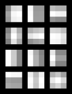
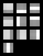
Figure 1: Experiments on bars data. Features: The $10$ original features that were used to construct the dataset. Data: A random sample of 12 data vectors. These constitute superpositions of the original features. NNSC: Features learned by NNSC, with dimensionality of the hidden representation equal to 10, starting from random initial values. NMF (6): Features learned by NMF, with dimensionality 6. NMF (10): Features learned by NMF, with dimensionality 10. See main text for discussion.

It is not difficult to understand why NMF cannot learn all the features. The data ${\bf X}$ can be perfectly described as an additive combination of the six single bars (because all double bars can be described as two single bars). Thus, NMF essentially achieves the optimum (zero reconstruction error) already with $6$ features, and there is no way in which an overcomplete representation could improve that. However, when sparseness is considered as in NNSC, it is clear that it is useful to have double bar features because these allow a sparser description of such data patterns.

In addition to these simulations, we have performed experiments with natural image data, reported elsewhere [3, 4]. These confirm our belief that sparseness is important when learning non-negative representations from data.

6 Relation to other work

In addition to the tight connection to linear sparse coding [2, 8] and non-negative matrix factorization [6, 7, 9], this method is intimately related to independent component analysis [5]. In fact, when the fixed-norm constraint is placed on the rows of ${\bf S}$ instead of the columns of ${\bf A}$, the objective (3) could be directly interpreted as the negative joint log-posterior of the basis vectors and components, given the data ${\bf X}$, in the noisy ICA model [4]. This connection is valid when the independent components are assumed to have exponential distributions, and of course the basis vectors are assumed to be non-negative as well.

Other researchers have also recently considered the constraint of non-negativity in the context of ICA. In particular, Plumbley [11] has considered estimation of the noiseless ICA model (with equal dimensionality of components and observations) in the case of non-negative components. On the other hand, Parra et al. [10] considered estimation of the ICA model where the basis (but not the components) was constrained to be non-negative. The main novelty of the present work is the application of the non-negativity constraints in the sparse coding framework, and the simple yet efficient algorithm developed to estimate the components.

7 Conclusions

In this paper, we have defined non-negative sparse coding as a combination of sparse coding with the constraints of non-negative matrix factorization. Although this is essentially a special case of the general sparse coding framework, we believe that the proposed constraints can be important for learning parts-based representations from non-negative data. In addition, the constraints allow a very simple yet efficient algorithm for estimating the hidden components.

8 Appendix

To prove Theorem 1, first note that the objective (3) is separable in the columns of ${\bf S}$ so that each column can be optimized without considering the others. We may thus consider the problem for the case of a single column, denoted ${\bf s}$. The corresponding column of ${\bf X}$ is denoted ${\bf x}$, giving the objective

$$F({\bf s})=\frac{1}{2}\|{\bf x}-{\bf A}{\bf s}\|^{2}+\lambda\sum_{i}s_{i}.$$ (5)

The proof will follow closely the proof given in [7] for the case $\lambda=0$. (Note that in [7], the notation $v={\bf x}$, $W={\bf A}$ and $h={\bf s}$ was used.) We define an auxiliary function $G({\bf s},{\bf s}^{t})$ with the properties that $G({\bf s},{\bf s})=F({\bf s})$ and $G({\bf s},{\bf s}^{t})\geq F({\bf s})$. We will then show that the multiplicative update rule corresponds to setting, at each iteration, the new state vector to the values that minimize the auxiliary function:

$${\bf s}^{t+1}=\arg\min_{{\bf s}}G({\bf s},{\bf s}^{t}).$$ (6)

This is guaranteed not to increase the objective function $F$, as

$$F({\bf s}^{t+1})\leq G({\bf s}^{t+1},{\bf s}^{t})\leq G({\bf s}^{t},{\bf s}^{t})=F({\bf s}^{t}).$$ (7)

Following [7], we define the function $G$ as

$$G({\bf s},{\bf s}^{t})=F({\bf s}^{t})+({\bf s}-{\bf s}^{t})^{T}\nabla F({\bf s}^{t})+\frac{1}{2}({\bf s}-{\bf s}^{t})^{T}{\bf K}({\bf s}^{t})({\bf s}-{\bf s}^{t})$$ (8)

where the diagonal matrix ${\bf K}({\bf s}^{t})$ is defined as

$$K_{ab}({\bf s}^{t})=\delta_{ab}\frac{({\bf A}^{T}{\bf A}{\bf s}^{t})_{a}+\lambda}{{\bf s}^{t}_{a}}.$$ (9)

It is important to note that the elements of our choice for ${\bf K}$ are always greather than or equal to those of the ${\bf K}$ used in [7], which is the case where $\lambda=0$. It is obvious that $G({\bf s},{\bf s})=F({\bf s})$. Writing out

$$F({\bf s})=F({\bf s}^{t})+({\bf s}-{\bf s}^{t})^{T}\nabla F({\bf s}^{t})+\frac{1}{2}({\bf s}-{\bf s}^{t})^{T}({\bf A}^{T}{\bf A})({\bf s}-{\bf s}^{t}),$$ (10)

we see that the second property, $G({\bf s},{\bf s}^{\prime})\geq F({\bf s})$, is satisfied if

$$0\leq({\bf s}-{\bf s}^{t})^{T}[{\bf K}({\bf s}^{t})-{\bf A}^{T}{\bf A}]({\bf s}-{\bf s}^{t}).$$ (11)

Lee and Seung proved this positive semidefiniteness for the case of $\lambda=0$ [7]. In our case, with $\lambda>0$, the matrix whose positive semidefiniteness is to be proved is the same except that a strictly non-negative diagonal matrix has been added (see the above comment on the choice of ${\bf K}$). As a non-negative diagonal matrix is positive semidefinite, and the sum of two positive semidefinite matrices is also positive semidefinite, the $\lambda=0$ proof in [7] also holds when $\lambda>0$.

It remains to be shown that the update rule in (4) selects the minimum of $G$. This minimum is easily found by taking the gradient and equating it to zero:

$$\nabla_{{\bf s}}G({\bf s},{\bf s}^{t})={\bf A}^{T}({\bf A}{\bf s}^{t}-{\bf x})+\lambda{\bf c}+{\bf K}({\bf s}^{t})({\bf s}-{\bf s}^{t})=0,$$ (12)

where ${\bf c}$ is a vector with all ones. Solving for ${\bf s}$, this gives

$${\bf s} = {\bf s}^{t}-{\bf K}^{-1}({\bf s}^{t})({\bf A}^{T}{\bf A}{\bf s}^{t}-{\bf A}^{T}{\bf x}+\lambda{\bf c})$$ (13)

$$= {\bf s}^{t}-({\bf s}^{t}./({\bf A}^{T}{\bf A}{\bf s}^{t}+\lambda{\bf c})).*({\bf A}^{T}{\bf A}{\bf s}^{t}-{\bf A}^{T}{\bf x}+\lambda{\bf c})$$ (14)

$$= {\bf s}^{t}.*({\bf A}^{T}{\bf x})./({\bf A}^{T}{\bf A}{\bf s}^{t}+\lambda{\bf c}))$$ (15)

which is the desired update rule (4). This completes the proof.

9 Acknowledgements

I wish to acknowledge Aapo Hyvärinen for useful discussions and helpful comments on an earlier version of the manuscript.

REFERENCES

- [1] G. F. Harpur, Low Entropy Coding with Unsupervised Neural Networks, Ph.D. thesis, University of Cambridge, 1997.
- [2] G. F. Harpur and R. W. Prager, “Development of low entropy coding in a recurrent network,” Network: Computation in Neural Systems, vol. 7, pp. 277–284, 1996.
- [3] P. O. Hoyer, “Modeling receptive fields with non-negative sparse coding,” Submitted. Available online, see http://www.cis.hut.fi/phoyer/papers/.
- [4] P. O. Hoyer and A. Hyvärinen, “A multi-layer sparse coding network learns contour coding from natural images,” Vision Research, In press. Available online, see http://www.cis.hut.fi/phoyer/papers/.
- [5] A. Hyvärinen, J. Karhunen and E. Oja, Independent Component Analysis, Wiley Interscience, 2001.
- [6] D. D. Lee and H. S. Seung, “Learning the parts of objects by non-negative matrix factorization,” Nature, vol. 401, no. 6755, pp. 788–791, 1999.
- [7] D. D. Lee and H. S. Seung, “Algorithms for non-negative matrix factorization,” in Advances in Neural Information Processing 13 (Proc. NIPS*2000), MIT Press, 2001.
- [8] B. A. Olshausen and D. J. Field, “Emergence of simple-cell receptive field properties by learning a sparse code for natural images,” Nature, vol. 381, pp. 607–609, 1996.
- [9] P. Paatero and U. Tapper, “Positive Matrix Factorization: A Non-negative Factor Model with Optimal Utilization of Error Estimates of Data Values,” Environmetrics, vol. 5, pp. 111–126, 1994.
- [10] L. Parra, C. Spence, P. Sajda, A. Ziehe and K.-R. Müller, “Unmixing Hyperspectral Data,” in Advances in Neural Information Processing 12 (Proc. NIPS*99), MIT Press, pp. 942–948, 2000.
- [11] M. Plumbley, “Conditions for non-negative independent component analysis,” IEEE Signal Processing Letters, Submitted.