Approximate Computation of Reach Sets in Hybrid Systems

Abstract

One of the most important problems in hybrid systems is the reachability problem. The reachability problem has been shown to be undecidable even for a subclass of linear hybrid systems. In view of this, the main focus in the area of hybrid systems has been to find effective semi-decision procedures for this problem. Such an algorithmic approach involves finding methods of computation and representation of reach sets of the continuous variables within a discrete state of a hybrid system. In this paper, after presenting a brief introduction to hybrid systems and reachability problem, we propose a computational method for obtaining the reach sets of continuous variables in a hybrid system. In addition to this, we also describe a new algorithm to over-approximate with polyhedra the reach sets of the continuous variables with linear dynamics and polyhedral initial set. We illustrate these algorithms with typical interesting examples.

1 Introduction

Hybrid systems combine discrete and continuous dynamics. The dynamics of the continuous variables within a discrete state are specified by differential equations or differential inclusions. An important problem in the analysis and sysnthesis of such systems is the so called reachability problem, which asks, for two sets of configurations of a given hybrid system, say ${\cal X}_{1}$ and ${\cal X}_{2}$, where a configuration consists of discrete and continuous components, whether or not there is a hybrid trajectory with the initial configuration in ${\cal X}_{1}$ and the final configuration in ${\cal X}_{2}$. A hybrid trajectory may be described as a trajectory of configurations consisting of discrete state jumps and smooth arcs, where each arc evolves according to the continuous dynamics of a discrete state, with the starting and end points of each arc satisfying the jump conditions of discrete transitions. A more precise definition is presented in Sec. 2, which provides a concise introduction to hybrid systems and the reachability problem.

The reachability problem is undecidable for certain classes of linear hybrid systems (i.e., hybrid systems having linear trajectories within each discrete state and linear or constant reset maps, also called constant slope hybrid systems) [1, 2], although in some cases decidability results have been obtained [3, 4] (see also [2]). Therefore, for a general hybrid system, a reasonable alternative appears to be to find semi-decision procedures for the reachability problem [5, 6, 7]. A computational approach to this problem also requires finding the set of states reached by the continuous variables evolving according to the dynamics of a discrete state. In this paper, we consider the problem of computing and representing the reach sets of the continuous variables within a discrete state when the dynamics of the continuous variables are specified by differential equations with initial conditions belonging to a specified initial set.

In this context, various methods have been proposed in the literature for finding reach sets of continuous variables [8, 9, 10]. In Sec. 3, we describe a method for computing the reach sets based on the idea that a subset of the boundary of the initial set may be found, such that it is sufficient to compute the solutions with the initial points lying in that set. This method is similar to that in [8] (and also to some extent to that described in [9]). In particular, we present a schematic algorithm, which is somewhat more general in its scope than that in [8] and simpler compared to that in [9].

Besides these algorithms for reach set computation, an equally important issue the representation of the reach sets for manipulating the sets efficiently. This requires representation of the reach sets in terms of more convenient sets such as, for example polyhedral or subalgebraic sets, that are simple to represent and easy to handle for practical purposes. However, since the representing class of sets may not contain a member that exactly equals the reach set, we may have to find approximations to the reach sets by those that belong to the representing class. (See, for example, [10, 12] for approximation with polyhedra, and [11] for approximation using ellipsoids). Typically, over-approximations may be used for verifying whether a safety requirement may potentially be violated by any of the behaviours starting from a given initial set, while under-approximations are needed for characterizing a set of states from which a desirable property is always achievable. We describe in Sec. 4 a method for over-approximating the reach sets by polyhedra when the dynamics are specified by linear differential equations and the initial set is a polyhedron. These algorithms are illustrated with some simple examples in Sec. 5, while Sec. 6 concludes the paper.

2 A Brief Survey of Hybrid Systems

In this section, we present a brief introduction to hybrid systems, and provide motivation for the remaining sections.

2.1 Preliminary Definitions

We begin with a somewhat detailed but general definition of hybrid systems.

Definition 1

A hybrid system is a tuple $H=(Q,X,\Sigma,G,E,Init,f)$, where

1. $Q$ is a finite set of discrete states (also called locations).

2. $X=\mathbb{R}^{n}$, $n\geq 1$, is the set of continuous states, where $\mathbb{R}$ denotes the set of real numbers. We demote the continuous state variable by $\mathbf{x}$.

3. $\Sigma$ is a finite set of discrete events or environment actions. Some events in $\Sigma$ are controllable, while others not. Hence, it is convenient to assume that $\Sigma=\Sigma_{c}\bigcup\Sigma_{d}$, where $\Sigma_{c}$ is the set of controllable events, and $\Sigma_{d}$ is the set of uncontrollable or disturbance events.

4. $G\subseteq Q\times X$ is a set of state invariance conditions. When the system is in state $q$, the continuous variables belong to $G(q)=\{\mathbf{x}\in X\,:\;(q,\mathbf{x})\in G\}$.

5. $E\subseteq Q\times{\cal P}(\mathbb{R}^{n})\times\Sigma\times\{\mathbb{R}^{n}\rightarrow\mathbb{R}^{n}\}\times Q$ is the set of transition edges. An edge $e\in E$, where $e=(q_{e},X_{e},\sigma_{e},r_{e},q^{\prime}_{e})$, is interpreted as follows:

   • If the continuous state is in $X_{e}$ and the event $\sigma_{e}$ occurs, then transition edge $e$ is enabled in state $q_{e}$. Thus $X_{e}$ is the set of switching points of the continuous variables from state $q_{e}$ to $q_{e}^{\prime}$. The set $X_{e}$ is specified by a predicate, and is also called a guard. In case there are many transition edges simultaneously enabled, then the system may select one of the edges nondeterministically.

   • If a transition edge $e$ is selected by the system, then the continuous state is reset using the function $r_{e}$ when the system enters state $q_{e}^{\prime}$. The reset values obey the state invariance condition, $r_{e}(X_{e})\subseteq G(q_{e}^{\prime})$.

6. $Init\subseteq G$ is a set of initial conditions.

7. $f$ is an $n$-dimensional vector field with real-valued components governing the dynamics of the continuous state $\mathbf{x}$. The domain of definition of the function $f$ is a set ${\cal D}$, where ${\cal D}=Q\times X$ (if there are no continuous control variables) or ${\cal D}=Q\times X\times U$ (if $U\subseteq\mathbb{R}^{m}$, $m\geq 1$, is the range of the continuous control variable, which is a function $\mathbf{u}:[0,T_{q})\rightarrow U$, where $T_{q}>0$ is as large as may be necessary, depending on the discrete state $q\in Q$). When in state $q$, the continuous variables evolve according to the dynamical law

   $$\frac{d\mathbf{x}}{dt}=f(q,\mathbf{x})$$

   or according to the dynamical law

   $$\frac{d\mathbf{x}}{dt}=f(q,\mathbf{x},\mathbf{u})$$

   depending on the presence or absence of the continuous control variables.

   The initial conditions of the continuous evolution are specified either by the reset maps when the system takes a discrete transition and reaches the state $q$, or by the (nondeterministic) initial conditions of the system given as the set $Init$.

If, in addition to the set of initial values, $Init$, the set of final or accepting values in $Q\times X$, denoted by $Final$, are also specified, then the hybrid system is called a hybrid automaton.

Referring to the system dynamics in the above definition, for our purposes, we assume that there are no continuous control variables. Therefore, in the sequel, we assume that the dynamics of the continuous variables are specified in the form

$$\frac{d\mathbf{x}}{dt}=f(q,\mathbf{x})$$

without any continuous control variables.

Definition 2

Let $H=(Q,X,\Sigma,G,E,Init,f)$ be a hybrid system. Each point $(q,\mathbf{x})\in Q\times X$ is called a configuration of the hybrid system $H$.

In Definitions 3 - 6, we introduce certain terminology, starting with the notion of a step of a hybrid system, leading upto the notions of predecessors and successors of a configuration $(q,\mathbf{x})$. But before that, we mention that predecessors and successors may be defined irrespective of initial conditions, whereas for defining the executions of a hybrid system, we require the specification of the initial set $Init$, as will be seen later (refer to Definitions 4, 5 and 6) .

Definition 3

Let $H=(Q,X,\Sigma,G,E,Init,f)$ be a hybrid system, and let $(q,\mathbf{x})$ and $(q^{\prime},\mathbf{x}^{\prime})$ be two configurations of $H$. Then, the pair of configurations $((q,\mathbf{x}),(q^{\prime},\mathbf{x}^{\prime}))$ is called

1. a time-step, if $q=q^{\prime}$ and, for some $t\geq 0$, there is a function $\mathbf{y}:[0,t]\rightarrow X$, satisfying $\dot{\mathbf{y}}(s)=f(q,\mathbf{y}(s))$, $\mathbf{y}(s)\in G(q)$, for $s\in[0,t]$, $\mathbf{y}(0)=\mathbf{x}$ and $\mathbf{y}(t)=\mathbf{x}^{\prime}$.

2. an edge-step if there is an edge $e=(q_{e},X_{e},\sigma_{e},r_{e},q_{e}^{\prime})\in E$, such that $q=q_{e}$, $q^{\prime}=q_{e}^{\prime}$, $\mathbf{x}\in X_{e}$ and $\mathbf{x}^{\prime}=r_{e}(\mathbf{x})$.

3. a $\sigma$-step, where $\sigma\in\Sigma$, if there is an edge $\ell=(q_{\ell},X_{\ell},\sigma_{\ell},r_{\ell},q_{\ell}^{\prime})\in E$ with $\sigma=\sigma_{\ell}$, such that $q=q_{\ell}$, $q^{\prime}=q_{\ell}^{\prime}$, $\mathbf{x}\in X_{\ell}$ and $\mathbf{x}^{\prime}=r_{\ell}(\mathbf{x})$.

A step of the hybrid system $H$ is a pair of configurations $((q,\mathbf{x}),(q^{\prime},\mathbf{x}^{\prime}))$, such that $((q,\mathbf{x}),(q^{\prime},\mathbf{x}^{\prime}))$ is either a time-step for some $t\geq 0$, or an edge-step for some $e\in E$, or a $\sigma$-step for some $\sigma\in\Sigma$.

Of course, every edge-step is a $\sigma$-step for some $\sigma\in\Sigma$, and conversely, every $\sigma$-step is an edge-step for some edge $e\in E$. Hence these definitions may seem redundant. However, the distinction between the two types of transitions would become obvious if there is a discrete state controller, defined as a function $C:Q\times X\rightarrow\Sigma_{c}$, that triggers discrete controllable events to enable a particular transition depending on the present configuration (see for instance [13] for the case of timed automata). But in this work, we shall not have occasion to discuss about discrete state controllers.

Definition 4

(Trajectories and Executions of a Hybrid System) A hybrid trajectory or simply a trajectory of $H$ is a sequence of configurations $(q_{1},\mathbf{x}_{1}),(q_{2},\mathbf{x}_{2}),(q_{3},\mathbf{x}_{3}),\ldots$, where for each $i\geq 1$, $((q_{i},\mathbf{x}_{i}),(q_{i+1},\mathbf{x}_{i+1}))$ is a step. A trajectory is

1. finite, if the number of steps is finite;

2. an execution, if $(q_{1},\mathbf{x}_{1})\in Init$, where $(q_{1},\mathbf{x}_{1})$ is the initial configuration; and

3. a finite execution, if it is both.

We now define, for each $\sigma\in\Sigma$, the set-valued successor function, $Post_{\sigma}:Q\times X\rightarrow 2^{Q}\times 2^{X}$. As will be briefly mentioned later (after Definition 6), our definitions lead in a natural way to extract a labeled transition system (see [14]) from a hybrid system.

Definition 5

($\sigma$-Successors of a Configuration)
Let $H=(Q,X,\Sigma,G,E,Init,f)$ be a hybrid system, $\sigma\in\Sigma$ and $(q,\mathbf{x})\in Q\times X$. Then, we define $Post_{\sigma}(q,\mathbf{x})$ to be the union of the two sets $S_{1},S_{2}^{\sigma}\subseteq Q\times X$, where

1. $S_{1}=\{(q^{\prime},\mathbf{x}^{\prime}):((q,\mathbf{x}),(q^{\prime},\mathbf{x}^{\prime}))\textrm{ is a time-step for some $t\geq 0$}\}$; and

2. $S_{2}^{\sigma}=\{(q^{\prime\prime},\mathbf{x}^{\prime\prime}):((q^{\prime},\mathbf{x}^{\prime}),(q^{\prime\prime},\mathbf{x}^{\prime\prime}))\textrm{ is a $\sigma$-step for some $(q^{\prime},\mathbf{x}^{\prime})\in S_{1}$ }\}$.

Further, if $(q_{s},\mathbf{x}_{s})\in Post_{\sigma}(q,\mathbf{x})$, then $(q_{s},\mathbf{x}_{s})$ is called a $\sigma$-successor of $(q,\mathbf{x})$.

The set $S_{1}$, as in the first part of this definition, is of main interest to us in the later sections of this paper. Specifically, we will deal with the set $Reach_{q}^{G}\left(X_{0}\right)$, where $q\in Q$ and $X_{0}\subseteq G(q)$, defined as

$$Reach_{q}^{G}\left(X_{0}\right)=\left\{\mathbf{x}:((q,\mathbf{x}_{0}),(q,\mathbf{x}))\textrm{ is a time-step for some}\textrm{ $t\geq 0$ and $\mathbf{x}_{0}\in X_{0}$ }\right\}.$$ (1)

In the subsequent sections, we will be concerned more with this and a related set. But for now, we shall proceed with our discussion with the following definition:

Definition 6

($\sigma$-Predecessors of a Configuration)
Let $H=(Q,X,\Sigma,G,E,Init,f)$ be a hybrid system, $\sigma\in\Sigma$ and $(q,\mathbf{x})\in Q\times X$. Then, we define $Pre_{\sigma}(q,\mathbf{x})$ to be the union of the two sets $P_{1},P_{2}^{\sigma}\subseteq Q\times X$, where

1. $P_{1}=\{(q^{\prime},\mathbf{x}^{\prime}):((q^{\prime},\mathbf{x}^{\prime}),(q,\mathbf{x}))\textrm{ is a time-step for some $t\geq 0$}\}$; and

2. $P_{2}^{\sigma}=\{(q^{\prime\prime},\mathbf{x}^{\prime\prime}):((q^{\prime\prime},\mathbf{x}^{\prime\prime}),(q^{\prime},\mathbf{x}^{\prime}))\textrm{ is a $\sigma$-step for some $(q^{\prime},\mathbf{x}^{\prime})\in P_{1}$ }\}$.

Further, if $(q_{p},\mathbf{x}_{p})\in Pre_{\sigma}(q,\mathbf{x})$, then $(q_{p},\mathbf{x}_{p})$ is called a $\sigma$-predecessor of $(q,\mathbf{x})$.

Note that the notion of $\sigma$-successor generalizes the notion of $\sigma$-step by including time-steps. The set valued function $Post_{\sigma}(q,\mathbf{x})$ defines, in a natural way, a transition relation, ${\hskip 1.42271pt\stackrel{{\scriptstyle\sigma}}{{\longrightarrow}}\hskip 1.42271pt}\subseteq(Q\times X)\times(Q\times X)$, as follows: $(q,\mathbf{x}){\hskip 1.42271pt\stackrel{{\scriptstyle\sigma}}{{\longrightarrow}}\hskip 1.42271pt}(q^{\prime},\mathbf{x}^{\prime})$, if $(q^{\prime},\mathbf{x}^{\prime})\in Post_{\sigma}(q,\mathbf{x})$. The transition relation ${\hskip 1.42271pt\stackrel{{\scriptstyle\sigma}}{{\longrightarrow}}\hskip 1.42271pt}$ is also called $\sigma$-transition relation. Similarly, the set valued function $Pre_{\sigma}(q,\mathbf{x})$ defines another transition relation, ${\hskip 1.42271pt\stackrel{{\scriptstyle\sigma}}{{\longleftarrow}}\hskip 1.42271pt}\subseteq(Q\times X)\times(Q\times X)$, as follows: $(q,\mathbf{x}){\hskip 1.42271pt\stackrel{{\scriptstyle\sigma}}{{\longleftarrow}}\hskip 1.42271pt}(q^{\prime},\mathbf{x}^{\prime})$, if $(q,\mathbf{x})\in Pre_{\sigma}(q^{\prime},\mathbf{x}^{\prime})$.

For two configurations $(q_{1},\mathbf{x}_{1})$ and $(q_{2},\mathbf{x}_{2})$, if $((q_{1},\mathbf{x}_{1}),(q_{2},\mathbf{x}_{2}))$ is a $\sigma$-step, then $(q_{2},\mathbf{x}_{2})\in Post(q_{1},\mathbf{x}_{1})$ and $(q_{1},\mathbf{x}_{1})\in Pre(q_{2},\mathbf{x}_{2})$; hence, in this case, we have $(q_{1},\mathbf{x}_{1}){\hskip 1.42271pt\stackrel{{\scriptstyle\sigma}}{{\longrightarrow}}\hskip 1.42271pt}(q_{2},\mathbf{x}_{2})$ and $(q_{1},\mathbf{x}_{1}){\hskip 1.42271pt\stackrel{{\scriptstyle\sigma}}{{\longleftarrow}}\hskip 1.42271pt}(q_{2},\mathbf{x}_{2})$. This may mislead us to get the false impression that ${\hskip 1.42271pt\stackrel{{\scriptstyle\sigma}}{{\longrightarrow}}\hskip 1.42271pt}$ and ${\hskip 1.42271pt\stackrel{{\scriptstyle\sigma}}{{\longleftarrow}}\hskip 1.42271pt}$ are the same; and to avoid any such possible confusion, we emphasize that, in general, it is not true that $(q_{1},\mathbf{x}_{1}){\hskip 1.42271pt\stackrel{{\scriptstyle\sigma}}{{\longrightarrow}}\hskip 1.42271pt}(q_{2},\mathbf{x}_{2})$ implies $(q_{1},\mathbf{x}_{1}){\hskip 1.42271pt\stackrel{{\scriptstyle\sigma}}{{\longleftarrow}}\hskip 1.42271pt}(q_{2},\mathbf{x}_{2})$; and the same with the converse statement. Hence, the two relations ${\hskip 1.42271pt\stackrel{{\scriptstyle\sigma}}{{\longrightarrow}}\hskip 1.42271pt}$ and ${\hskip 1.42271pt\stackrel{{\scriptstyle\sigma}}{{\longleftarrow}}\hskip 1.42271pt}$ are not the same.

The definitions of $Post_{\sigma}$ and $Pre_{\sigma}$ can be extended straightforwardly to subsets of $Q\times X$, as follows: for $S\subseteq Q\times X$, define

$$Post_{\sigma}(S)=\bigcup_{(q,\mathbf{x})\in S}Post_{\sigma}(q,\mathbf{x}),~{}\textrm{ and }~{}Pre_{\sigma}(S)=\bigcup_{(q,\mathbf{x})\in S}Pre_{\sigma}(q,\mathbf{x}).$$

Finally, define

$$Post(S)=\bigcup_{\sigma\in\Sigma}Post_{\sigma}(S),~{}\textrm{ and }~{}Pre(S)=\bigcup_{\sigma\in\Sigma}Pre_{\sigma}(S).$$

We sometimes refer to $Post$ and $Pre$ as the 1-step transition functions. More generally, the $k$-step transition functions $Post^{k}$ and $Pre^{k}$ are defined inductively as follows: For $S\subseteq Q\times X$,

$$Post^{1}(S)=Post(S),~{}\textrm{ and for $k\geq 2$, }~{}Post^{k}(S)=Post(Post^{k-1}(S)).$$

Similarly,

$$Pre^{1}(S)=Pre(S),~{}\textrm{ and for $k\geq 2$, }~{}Pre^{k}(S)=Pre(Pre^{k-1}(S)).$$

Finally, define $Post^{*}$ and $Pre^{*}$ as

$$Post^{*}(S)=\bigcup_{k\geq 1}Post^{k}(S),~{}\textrm{ and }~{}Pre^{*}(S)=\bigcup_{k\geq 1}Pre^{k}(S).$$

2.2 Reachability Problem for Hybrid Systems

In the notation just discussed, the reachability problem for a hybrid system $H=(Q,X,\Sigma,G,E,Init,f)$, where $Init$ is not necessarily specified in advance, may be posed as follows:

ReachProblem1:  For two subsets $S_{1}$ and $S_{2}$ of $Q\times X$, is there a finite

trajectory, $(q_{1},\mathbf{x}_{1}),(q_{2},\mathbf{x}_{2}),\ldots,(q_{N},\mathbf{x}_{N})$, for some

$N\geq 1$, such that $(q_{1},\mathbf{x}_{1})\in S_{1}$ and $(q_{N},\mathbf{x}_{N})\in S_{2}$ ?

This may also be rephrased as

ReachProblem2:	For two subsets $S_{1}$ and $S_{2}$ of $Q\times X$,
	whether $Post^{*}(S_{1})\bigcap S_{2}\neq\emptyset$ ?
	equivalently: whether $S_{1}\bigcap Pre^{*}(S_{2})\neq\emptyset$ ?

If the initial set $Init$ is specified in advance, then, with $S_{1}=Init$, the reachability problem ReachProblem1 becomes

ReachProblem3:	For a subset $S$ of $Q\times X$,
	is there a finite execution of $H$
	with final configuration in $S$ ?

There is a counterpart to the reachability problem, called the avoidance problem, which may be posed as follows:

AvoidProblem:	For two subsets $S_{1}$ and $S_{2}$ of $Q\times X$,
	whether $Post^{*}(S_{1})\bigcap S_{2}=\emptyset$ ?
	equivalently: whether $S_{1}\bigcap Pre^{*}(S_{2})=\emptyset$ ?

In the sequel, we restrict our attention to ReachProblem1 or ReachProblem2. We observe that the answers to these questions depend, in general, not only on the hybrid system $H$, but also on the class ${\cal C}$ of subsets of $Q\times X$ that are under consideration. Informally, the class ${\cal C}$ is required to

1. include a specified class of sets ${\cal S}$, where ${\cal S}$ may consist of the initial set, sets defined by state invariance conditions, those defined by guard conditions, and domains and ranges of reset maps of edges (and also final sets, if specified),

2. be closed under the boolean set operations of union and complimentation, and under the functions $Post_{\sigma}$ and $Pre_{\sigma}$, and

3. have an effective decision procedure for answering questions such as, for two sets $S_{1},S_{2}\in{\cal C}$, whether $S_{1}=S_{2}$ or not.

A formal presentation of these notions is beyond the scope of this work, although a brief discussion may be found in Appendix A. For more details, the interested reader may refer to the references on Model Theory, such as [19, 20, 21, 22]. But, for our purposes, we will be content with the following (somewhat informal) definition:

Definition 7

An algorithm for the reachability problem is said to be

1. a decision procedure, if the algorithm stops after a finite number of steps with the correct answer, where the answer can be either yes or no.

2. a semi-decision procedure, if the algorithm

   1. never stops with an incorrect answer, and

   2. always stops after a finite number of steps with the correct answer, whenever the answer is yes.

A hybrid system $H$ is decidable, if there is a decision procedure for the reachability problem for $H$.

Obviously, for a hybrid system $H$, if there are semi-decision procedures for both reachability problem and avoidance problem, then $H$ is decidable.

We describe below a schematic semi-decision procedure for the reachability problem of a hybrid system:

Semi-Decision Procedure for ReachProblem2

Input : Sets $S_{1}$ and $S_{2}$ Output : “yes”, if there is a trajectory from $S_{1}$ to $S_{2}$

Initialization $S:=S_{1}$

while $S\bigcap S_{2}=\emptyset$ do

$S:=Post(S)$

end while

return “yes”

In the later part of this section, we shall be mainly concerned with the computational aspects of the $Post$-operator appearing in the while-loop of the above schematic.

2.3 Computation of the $Post$-operator

We describe here a computational approach to finding $Post(S)$, $S\subseteq Q\times\mathbb{R}^{n}$, as in the semi-decision procedure for ReachProblem2 discussed in Sec. 2.2. Recall that, within a discrete state $q\in Q$, the continuous dynamics of $\mathbf{x}$ are specified by

$$\frac{d\mathbf{x}}{dt}=f(q,\mathbf{x})$$ (2)

with the initial conditions $\mathbf{x}(0)=\mathbf{x}_{0}\in X_{0}\subseteq X=\mathbb{R}^{n}$. We begin our discussion with the following definition.

Definition 8

Let $\mathbb{R}^{+}$ denote the set of nonnegative real numbers. Then, for each discrete state $q\in Q$, the flow associated with equation (5) is a function $\phi_{q}:\mathbb{R}^{n}\times\mathbb{R}^{+}\rightarrow\mathbb{R}^{n}$, defined as $\phi_{q}(\mathbf{x},t)=\gamma_{\mathbf{x}}(t)$, $t\geq 0$ and $\mathbf{x}\in\mathbb{R}^{n}$, where the function $\gamma_{\mathbf{x}}:\mathbb{R}^{+}\rightarrow\mathbb{R}^{n}$ satisfies

$$\frac{d\gamma_{\mathbf{x}}(t)}{dt}=f(q,\gamma_{\mathbf{x}}(t)),$$

with the initial condition $\gamma_{\mathbf{x}}(0)=\mathbf{x}$.

Recall the set of reachable phases $Reach_{q}^{G}$ as defined in (1). In the following definition, the same is defined in terms of the flow function $\phi_{q}$:

Definition 9

Let $q\in Q$ and $X_{0}\subset\mathbb{R}^{n}$. Then, the set of reachable continuous phases in the state $q$, is the set $Reach_{q}^{G}\left(X_{0}\right)$ defined as

$$Reach_{q}^{G}(X_{0}) = \left\{\mathbf{x}\in\mathbb{R}^{n}:~{}\exists\mathbf{x}_{0}\in X_{0}\;\exists t\geq 0\textrm{ $\mathbf{x}=\phi_{q}(\mathbf{x}_{0},t)$ and}\right.$$ (3)

$$\indent\left.\forall s~{}0\leq s\leq t\Rightarrow\phi_{q}(\mathbf{x}_{0},s)\in G(q)\right\}$$

We now define another operator, called the projection operator, as follows:

Definition 10

Let $S\subseteq Q\times X$. Then, the projection of S on X, is the set $\pi_{{}_{X}}(S)=\{\mathbf{x}\in X:\;(q,\mathbf{x})\in S\}$.

In terms of the operators $\pi_{{}_{X}}$ and $Reach_{q}^{G}$, the operator $Post$ may be rewritten as

$$Post(S)=\mathop{\bigcup_{e=(q_{e},X_{e},\sigma_{e},r_{e},q^{\prime}_{e})\in E,\;q=q_{e}}}_{X_{e}\bigcap\;[Reach_{q}^{G}\;\circ\;\pi_{{}_{X}}(S)]\hskip 1.42271pt\neq\emptyset}~{}~{}\{q_{e}^{\prime}\}\times[r_{e}\hskip 1.42271pt\circ\hskip 1.42271ptReach_{q}^{G}\hskip 1.42271pt\circ\hskip 1.42271pt\pi_{{}_{X}}(S)],$$ (4)

where, for two operators $g$ and $h$, $g\circ h$ is the composition of the two operators. With regard to computational issues, the set operators $\pi_{{}_{X}}$ and $r_{e}$ may not pose difficulties (provided $r_{e}$ is suitably specified). Hence the problem reduces to that of computation of $Reach_{q}^{G}$, and effectively representing the resulting set. Referring to the definition of $Reach_{q}^{G}$ as in (3), the significant and challenging task is the elimination of quantifiers, whenever possible. But, as shown in [23], not all theories of the real number system may admit quantifier elimination (see also the discussion presented in [15] and in Appendix A). This fact provides a motivation for the study of alternative methods (without requiring quantifier elimination method) for computating the set $Reach_{q}^{G}(X_{0})$.

Specifically, in the remaining part of the work, we shall be concerned with computation of the operator $Reach_{q}^{G}$ and with representation of the resulting sets. Below is a concise description of the questions that we shall be interested in and of the organization of the rest of the paper:

1. How to effectively compute the set operator $Reach_{q}^{G}$, at least when the global invariance condition is not imposed but a time bound is specified? In this case, we are interested in the set $Reach_{q}(X_{0},[0,\tau])$, $\tau\geq 0$, $X_{0}\subset\mathbb{R}^{n}$, defined as

   $$Reach_{q}(X_{0},[0,\tau])=\left\{\mathbf{x}\in\mathbb{R}^{n}:~{}\exists\mathbf{x}_{0}\in X_{0}\;\exists t\;0\leq t\leq\tau\textrm{ and }\mathbf{x}=\phi_{q}(\mathbf{x}_{0},t)\right\}.$$

   In Sec. 3, we present a schematic algorithm for computing $Reach_{q}(X_{0},[0,\tau])$. This algorithm is based on a generalization of the method described in [8].

2. How to compute – either exactly or approximately – the set operator $Reach_{q}^{G}$ when the global invariance condition is imposed (without time bound). In this case, we have to deal with the set operator $Reach_{q}^{G}$ as defined in (3), and obviously, it would be best to find an algorithm based on quantifier elimination. But, as mentioned earlier, we do not assume that quantifier elimination method is feasible, hence we may have to find an algorithm that computes an approximation to $Reach_{q}^{G}$. In Sec. 3, we indicate how to extend the algorithm for computing $Reach_{q}(X_{0},[0,\tau])$, as mentioned above, to compute an under-approximation or an over-approximation (depending on which one is preferred) to the set $Reach_{q}^{G}(X_{0})$.

3. Finally, how to represent the reach sets obtained by the operators $Reach_{q}$ and $Reach_{q}^{G}$, i.e. the sets $Reach_{q}(X_{0},[0,\tau])$ or $Reach_{q}^{G}(X_{0})$ as the case may be, such that boolean set operations such as union and complementation can be performed efficiently. This requires represention of the reach sets in terms of sets that are simple and easy to handle, such as polyhedral sets and subalgebraic sets. In [12], an algorithm algorithm for over-approximating the reach sets using polyhedral sets is presented. In Sec. 4, we describe another algorithm for over-approximating the reach sets with polyhedral sets. The algorithm presented in this paper differs from that of [12], but if these two methods – that described in Sec. 4 and that of [12] – are used together, then better results of over-approximation may be obtained.

The remaining part of the paper is orgainized as follows. In Sec. 3 and Sec. 4, we restrict our attention to these issues. We illustrate these algorithms with simple examples in Sec. 5, while Sec. 6 summarizes the paper.

3 Computational Approaches for Finding Reach Sets

3.1 Preliminary Discussion on Reach Sets

Let $H=(Q,X,\Sigma,G,E,Init,f)$ be a hybrid system. For $q\in Q$, consider the equation

$$\frac{d\mathbf{x}}{dt}=f(q,\mathbf{x})$$ (5)

with the initial conditions $\mathbf{x}(0)=\mathbf{x}_{0}\in X_{0}\subset X=\mathbb{R}^{n}$. It is customary to assume that $f(q,\cdot)$ is Lipschitz continuous in the second variable, in order to ensure existence and uniquness of solutions to the system of differential equations in (5). Further, we assume that the initial set $X_{0}$ is closed. Let, as before, the flow (refer to Defintion 8) associated with (5) be $\phi_{q}(\mathbf{x},t)$ and let $Reach_{q}(X_{0},t)=\{\phi_{q}(\mathbf{x}_{0},t):\mathbf{x}_{0}\in X_{0}\}$ be the set of phases reached at time $t\geq 0$ in state $q$ with initial conditions in $X_{0}$. Further, let

$$Reach_{q}(X_{0},[0,\tau]) = \bigcup_{0\leq t\leq\tau}Reach_{q}(X_{0},t),~{}~{}~{}~{}\tau\geq 0,$$

$$Reach_{q}(X_{0},[0,\infty)) = \bigcup_{\tau>0}Reach_{q}(X_{0},[0,\tau]).$$

We shall now define, for a set $X_{q}$, such that $X_{0}\subseteq X_{q}\subseteq\mathbb{R}^{n}$, another set $Reach_{q}^{\prime}\left(X_{0},X_{q},\,[0,\infty)\right)$. For this purpose, we first define, for each $\mathbf{x}\in X_{0}$, a number $\tau_{\mathbf{x}}$ as follows:

$$\tau_{\mathbf{x}}=\inf\{t>0\hskip 1.42271pt:\phi_{q}(\mathbf{x},t)\not\in X_{q}\},$$ (6)

where we assume that if $\tau_{\mathbf{x}}=\infty$, then $\phi_{q}(\mathbf{x},\infty)$ denotes the set of all $\omega$-limit points (see, for instance, [17]) of $\phi_{q}(\mathbf{x},t)$, for $t\geq 0$, and

$$\{\phi_{q}(\mathbf{x},t):0\leq t\leq\infty\}=\{\phi_{q}(\mathbf{x},t):0\leq t<\infty\}\bigcup\phi(\mathbf{x},\infty).$$

Further, let $\Theta_{q}(\mathbf{x},X_{q})\subseteq\mathbb{R}^{n}$ be defined as follows:

$$\Theta_{q}(\mathbf{x},X_{q})=\left\{\begin{array}[]{l}\{\phi_{q}(\mathbf{x},t)\hskip 1.42271pt:0\leq t\leq\tau_{\mathbf{x}}\},~{}~{}\textrm{if $\tau_{\mathbf{x}}<\infty$ and $\phi(\mathbf{x},\tau_{\mathbf{x}})\in X_{q}$,}\\ \{\phi_{q}(\mathbf{x},t)\hskip 1.42271pt:0\leq t\leq\infty\},~{}~{}\textrm{if $\tau_{\mathbf{x}}=\infty$ and $\phi(\mathbf{x},\infty)\subseteq X_{q}$,}\\ \{\phi_{q}(\mathbf{x},t)\hskip 1.42271pt:0\leq t<\tau_{\mathbf{x}}\},~{}~{}\textrm{otherwise.}\end{array}\right.$$

Then the set $Reach_{q}^{\prime}\left(X_{0},X_{q},\,[0,\infty)\right)$ is defined as

$$Reach_{q}^{\prime}\left(X_{0},X_{q},\,[0,\infty)\right)=\bigcup_{\mathbf{x}\in X_{0}}\Theta_{q}(\mathbf{x},X_{q}).$$

Now, by taking $X_{q}=G(q)$ in the above definition, we have

$$Reach_{q}^{G}\left(X_{0}\right)=Reach_{q}^{\prime}\left(X_{0},X_{q},\,[0,\infty)\right),$$

where $Reach_{q}^{G}\left(X_{0}\right)$ is defined as in (3), reproduced below for convenience:

$$Reach_{q}^{G}(X_{0}) = \left\{\mathbf{x}\in\mathbb{R}^{n}:~{}\exists\mathbf{x}_{0}\in X_{0}\;\exists t\geq 0\textrm{ $\mathbf{x}=\phi_{q}(\mathbf{x}_{0},t)$ and}\right.$$

$$\indent\left.\forall s~{}0\leq s\leq t\Rightarrow\phi_{q}(\mathbf{x}_{0},s)\in G(q)\right\}$$

Throughout the rest of the discussion, we fix a state $q$, and consider the problem of computing the sets $Reach_{q}(X_{0},[0,\tau])$ and $Reach_{q}^{\prime}\left(X_{0},X_{q},\,[0,\infty)\right)$.

3.2 A Computational Method: Generalized Face-Lifting Algorithm

When $X_{0}$ is suitably specified (such as, for example, a rectangle), this problem may be solved by finding the solutions to (5) with $\mathbf{x}(0)$ on the boundary of $X_{0}$. This results in evolving the boundary of $X_{0}$. More precisely, let $S_{0}$ be the boundary of $X_{0}$, and $X(\tau)=X_{0}\bigcup_{0\leq t\leq\tau}\{\phi_{q}(\mathbf{x}_{0},t):\mathbf{x}_{0}\in S_{0}\}$. Then $X(\tau)=Reach_{q}(X_{0},[0,\tau])$ (see Appendix A for a proof). This is the idea underlying the computational approach, called face lifting method, described in [8]. In this section, we shall study this in considerably more general setting, and describe an algorithm, called generalized face lifting method. It may be noted that the method described in [8] does not assume that a global invarience requirement is imposed; hence the algorithm of [8] computes only $Reach_{q}(X_{0},[0,\tau])$. However, we shall extend our method for computing $Reach_{q}(X_{0},[0,\tau])$ for computing an approximation to the set $Reach_{q}^{G}(X_{0})$, where the approximation can chosen to be either under-approximation or over-approximation.

Further, let $S_{0}^{+}\subseteq S_{0}$ be the set of those boundary points of $X_{0}$, such that the solution with initial point in $S_{0}^{+}$ extends into $X_{0}^{c}\;{\small{\stackrel{{\scriptstyle\Delta}}{{=}}}}\;\mathbb{R}^{n}\backslash X_{0}$ , i.e.,

$$S_{0}^{+}=\{\mathbf{x}_{0}\in S_{0}\hskip 1.42271pt:\exists\epsilon\;=\;\epsilon(\mathbf{x}_{0})>0\textrm{ such that }\phi_{q}(\mathbf{x}_{0},t)\in X_{0}^{c},~{}\forall t\in(0,\epsilon)\},$$ (7)

and define $X^{+}(\tau)=X_{0}\bigcup_{0\leq t\leq\tau}\{\phi_{q}(\mathbf{x}_{0},t)\hskip 1.42271pt:\;\mathbf{x}_{0}\in S_{0}^{+}\}$. It turns out that $X^{+}(\tau)=X(\tau)=Reach_{q}(X_{0},[0,\tau])$ (see Appendix A). Therefore, in order to find $Reach_{q}(X_{0},[0,\tau])$, we have to find only those solutions for which the initial conditions are in $S_{0}^{+}$.

If $S_{0}^{+}$ can be found explicitly (by inspection of $\mathbf{f}$ and $S_{0}$), then the problem reduces justifiably to finding the solutions with initial conditions in $S_{0}^{+}$. Otherwise, we may have to find a means of obtaining an outer approximation to $S_{0}^{+}$, i.e., a set $S_{1}^{+}$ satisfying $S_{0}^{+}\subseteq S_{1}^{+}\subseteq S_{0}$. We suggest a way to find such a set. For this purpose, we assume that $X_{0}$ is specified as follows: there is a continuously differentiable function, $\ell:\mathbb{R}^{n}\rightarrow\mathbb{R}$, such that if $\mathbf{x}\in{\stackrel{{\scriptstyle\circ}}{{X_{0}}}}$ then $\ell(\mathbf{x})<0$ (where ${\stackrel{{\scriptstyle\circ}}{{X_{0}}}}$ denotes the interior of $X_{0}$, i.e., the largest open set contained in $X_{0}$), and if $\mathbf{x}\in X_{0}^{c}$ then $\ell(\mathbf{x})>0$. Hence $\ell(\mathbf{x})=0$ on $S_{0}$. Define

$$S_{1}^{+}=\{\mathbf{x}\in S_{0}\hskip 1.42271pt:~{}\nabla\ell(\mathbf{x})\cdot f(q,\mathbf{x})\geq 0\}.$$

It may be easily shown that $S_{0}^{+}\subseteq S_{1}^{+}$ (see Appendix A). Futher, we observe that the set of points for which $\nabla\ell(\mathbf{x})\cdot f(q,\mathbf{x})>0$, constitutes an inner approximation to $S_{0}^{+}$. The method of finding an $S_{1}^{+}$ as described above can be extended easily to the situation where $X_{0}$ is specified as the set of intersection of finitely many sets of the form $\ell_{i}(\mathbf{x})\leq 0$, with the strict inequality in ${\stackrel{{\scriptstyle\circ}}{{X_{0}}}}$.

With this notation, we proceed to describe a schematic algorithm for finding $X^{+}(\tau)$ for $\tau\geq 0$. In order to exploit the semigroup property of the reach set, i.e., $Reach_{q}(X_{0},[0,t])=Reach_{q}(Reach_{q}(X_{0},[0,s]),[0,t-s])$, for any $t$ and $s$, with $0\leq s\leq t$, we consider a sequence of time intervals $[0,\tau_{1}]$, $[\tau_{1},\tau_{2}]$, $[\tau_{2},\tau_{3}]$, etc., where $0<\tau_{1}<\tau_{2}<\tau_{3}<\ldots$, and $\tau_{i}\rightarrow\infty$, as $i\rightarrow\infty$. It may be convenient to choose for some $\tau>0$, $\tau_{i}=i\tau$, $i=0,1,2,\ldots$, although we do not require such an assumption in the algorithm.

Procedure for $Reach_{q}\left(X_{0},[0,\tau]\right)$

initialize: $X^{+}(0):=X_{0}$, $F_{0}:=S_{1}^{+}$ and $i:=0$

while $\tau>\tau_{i}$ and $F_{i}\neq\emptyset$ do

if $\tau<\tau_{i+1}$ then $\Delta_{i}:=\tau-\tau_{i}$ else $\Delta_{i}:=\tau_{i+1}-\tau_{i}$  end if

$T_{i}:=\{\phi_{q}(\mathbf{x},t)\,:~{}t\in[0,\Delta_{i}],~{}\mathbf{x}\in F_{i}\}$

/* this computational step requires special attention! */

$X^{+}(\tau_{i}+\Delta_{i}):=X^{+}(\tau_{i})\bigcup T_{i}$

$F_{i+1}:=\{\phi(\mathbf{x},\Delta_{i})\,:~{}\mathbf{x}\in F_{i}\}\backslash X^{+}(\tau_{i})$

$i:=i+1$

end while

In the above schematic, the initialization step “$F_{0}:=S_{1}^{+}$” could be replaced with “$F_{0}:=S_{0}^{+}$”, as it is not necessary to initialize $F_{0}$ to $S_{1}^{+}$. However, before proceeding further, it must be mentioned that with reference to this algorithm, we assume that the computational steps “$T_{i}:=\{\phi_{q}(\mathbf{x},t)\,:~{}t\in[0,\Delta_{i}],~{}\mathbf{x}\in F_{i}\}$” and “$F_{i+1}:=\{\phi(\mathbf{x},\Delta_{i})\,:~{}\mathbf{x}\in F_{i}\}\backslash X^{+}(\tau_{i})$” can be performed effectively.

We now describe a method for extending this procedure to another procedure that computes an approximation to $Reach_{q}^{\prime}(X_{0},X_{q},[0,\infty))$. But since $Reach_{q}^{G}(X_{0})=Reach^{\prime}(X_{0},G(q),[0,\infty))$, the procedure to be described below finds an approximation to $Reach_{q}^{G}(X_{0})$, when $X_{q}=G(q)$. The approximation can be chosen to be either under-approximation or over-approximation, depeding on a flag “$under\_approximate$”, passed as input to the algorithm (refer to the schematic algorithm described below).

To facilitate the discussion, we consider the flow $\psi_{q}(\mathbf{x},t)$, $t\geq 0$, $\mathbf{x}\in X=\mathbb{R}^{n}$, corresponding to the differential equation

$$\frac{d\mathbf{x}}{dt}=-f(q,\mathbf{x})$$ (8)

with the initial conditions $\mathbf{x}(0)=\mathbf{x}_{0}\in X=\mathbb{R}^{n}$. Now since the flow $\psi_{q}$ has the opposite direction to that of $\phi_{q}$, for any $t\geq 0$ and two subsets $X_{1}$ and $X_{2}$ of $\mathbb{R}^{n}$, we have, $X_{2}=\phi_{q}(X_{1},t)$ if and only if $X_{1}=\psi_{q}(X_{2},t)$. The function $\psi_{q}$ will be used in the procedure for computing an approximation to $Reach^{\prime}(X_{0},X_{q},[0,\infty))$, for finding, in each iteration, the set of initial conditions in $F_{i}$ corresponding to which the solutions for the time interval $[0,\Delta_{i}]$ may violate the global invariance requirement. With this, we present the schematic algorithm as follows:

Procedure for $Reach_{q}^{\prime}\left(X_{0},X_{q},[0,\infty)\right)$

precondition: $X_{0}\subseteq X_{q}$

boolean input flag: $under\_approximate$

/* $under\_approximate=1$, if under-approximation is preferred */

/* by default, the procedure over-approximates the reach set */

initialize: $X^{+}(0):=X_{0}$, $F_{0}:=S_{1}^{+}$ and $i:=0$

while $F_{i}\neq\emptyset$ do

$\Delta_{i}:=\tau_{i+1}-\tau_{i}$

$T_{i}:=\{\phi_{q}(\mathbf{x},t)\,:~{}t\in[0,\Delta_{i}],~{}\mathbf{x}\in F_{i}\}$

if $T_{i}\subseteq X_{q}$ then    /* global invariance not violated */

$X^{+}(\tau_{i}+\Delta_{i}):=X^{+}(\tau_{i})\bigcup T_{i}$

$F_{i+1}:=\{\phi_{q}(\mathbf{x},\Delta_{i})\,:~{}\mathbf{x}\in F_{i}\}\backslash X^{+}(\tau_{i})$

else     /* global invariance violated by at least one trajectory */

$U_{i}:=T_{i}\backslash X_{q}$

$V_{i}:=\{\psi_{q}(\mathbf{x},t):~{}t\in[0,\Delta_{i}],~{}\mathbf{x}\in U_{i}\}$

$F_{i}^{\prime}=F_{i}\backslash V_{i}$

$T_{i}^{\prime}:=\{\phi_{q}(\mathbf{x},t)\,:~{}t\in[0,\Delta_{i}],~{}\mathbf{x}\in F_{i}^{\prime}\}$

if $under\_approximate=1$ then

$X^{+}(\tau_{i}+\Delta_{i}):=X^{+}(\tau_{i})\bigcup U_{i}$

else

$X^{+}(\tau_{i}+\Delta_{i}):=X^{+}(\tau_{i})\bigcup T_{i}^{\prime}$

end if

$F_{i+1}:=\{\phi_{q}(\mathbf{x},\Delta_{i})\,:~{}\mathbf{x}\in F_{i}^{\prime}\}\backslash X^{+}(\tau_{i})$

end if

$i:=i+1$

end while

As with the previous algorithm, the initialization step “$F_{0}:=S_{1}^{+}$” could be replaced with “$F_{0}:=S_{0}^{+}$”, depending on convenience. Termination of this procedure may be guaranteed, if certain assumptions are satisfied. The required assumptions are as follows:

1. the set $Y_{q}=\overline{X_{q}}$ is compact;

2. $X_{0}$ is closed in $\mathbb{R}^{n}$; and

3. for every $\mathbf{x}_{0}\in X_{0}$, $Y_{q}$ does not contain any $\omega$-limit points of the trajectory of $\phi_{q}(\mathbf{x}_{0},t)$, $t\geq 0$, more precisely,

   $$\phi_{q}(\mathbf{x}_{0},\infty)\bigcap Y_{q}=\emptyset,~{}~{}\mathbf{x}_{0}\in X_{0}.$$

Under these assumptions, it can be shown that (see Appendix C) there is a $\tau_{\max}>0$, such that for every $\mathbf{x}\in X_{0}$, there is a $\tau(\mathbf{x})>0$ with $0<\tau(\mathbf{x})\leq\tau_{max}$ and $\phi_{q}(\mathbf{x},\tau(\mathbf{x}))\not\in X_{q}$. Obviously, with such a $\tau_{\max}$, we have $\tau_{\mathbf{x}}\leq\tau_{\max}$, for each $\mathbf{x}\in X_{0}$, where $\tau_{\mathbf{x}}$ is as in (6). Termination of the algorithm may be deduced from this as follows: Consider a sequence of sets $F_{0}^{(i)}$, $i\geq 0$, defined as $F_{0}^{(i)}=\{\mathbf{x}\in S_{0}:\phi_{q}(\mathbf{x},\tau_{i})\in F_{i}\}$. It is easy to check that $F_{0}^{(i)}$ is a nonincreasing sequence of sets, i.e., $F_{0}^{(i+1)}\subseteq F_{0}^{(i)}$. Let $\mathbf{x}\in X_{0}$, and let $k$ be a nonnegative integer such that $\tau_{k}\leq\tau_{\mathbf{x}}<\tau_{k+1}$. Now, during the $k$’th iteration of the while-loop, the global invariance condition (the condition that $T_{k}\subseteq X_{q}$) is violated, since $\phi_{q}(\mathbf{x},t)\not\in X_{q}$, for some $t$ such that $\tau_{\mathbf{x}}\leq t<\tau_{k+1}$. Let $\tau_{\mathbf{x}}^{\prime}\in[\tau_{\mathbf{x}},\tau_{k+1})$ be a time instant such that $\phi_{k}(\mathbf{x},\tau_{\mathbf{x}}^{\prime})\not\in X_{0}$, and let $t_{\mathbf{x}}=\tau_{\mathbf{x}}^{\prime}-\tau_{k}$. With this choice of $t_{\mathbf{x}}$, we have both $0\leq t_{\mathbf{x}}<\Delta_{k}$ and $\phi_{q}(\mathbf{x},\tau_{k}+t_{\mathbf{x}})\not\in X_{q}$. Thus, $\phi_{q}(\mathbf{x},\tau_{k}+t_{\mathbf{x}})\in U_{k}=T_{k}\backslash X_{q}$ (refer to the schematic above). Let $\mathbf{y}=\phi_{q}(\mathbf{x},\tau_{k}+t_{\mathbf{x}})$, so $\phi_{q}(\mathbf{x},\tau_{k})=\psi_{q}(\mathbf{y},t_{\mathbf{x}})$. But, since $\mathbf{y}\in U_{k}$, $\psi_{q}(\mathbf{y},t_{\mathbf{x}})\in V_{k}$ (refer to the schematic). Hence $\phi_{q}(\mathbf{x},\tau_{k})\in V_{k}$ and $\phi_{q}(\mathbf{x},\tau_{k})\not\in F_{k}^{\prime}=F_{k}\backslash V_{k}$. Therefore $\phi_{q}(\mathbf{x},\tau_{k+1})\not\in F_{k+1}$, implying that $\mathbf{x}\not\in F_{0}^{(k+1)}$. By the monotonicity of the sequence of sets $F_{0}^{(i)}$, we have $\mathbf{x}\not\in F_{0}^{(i)}$, for any $i\geq k+1$. Finally, let $m\geq 0$ be an integer such that $\tau_{m}\leq\tau_{\max}<\tau_{m+1}$. Now since $\tau_{\mathbf{x}}\leq\tau_{\max}$, $\mathbf{x}\not\in F_{0}^{(m+1)}$, for any $\mathbf{x}\in X_{0}$. Hence $F_{0}^{(m+1)}=\emptyset$, so $F_{m+1}=\emptyset$, satisfying the terminating condition of the while-loop of the algorithm, after at most $m$ number of iterations.

In the rest of the paper, we discuss approximation of the set $T_{i}$ appearing in the second line of the while-loop of the above schematic (see also the schematic for $Reach(X_{0},[0,\tau])$), when $f(q,\mathbf{x})$ is of the form $f(q,\mathbf{x})=A_{q}\mathbf{x}$, where $A_{q}$ is a constant $n\times n$ matrix with real entries and the initial set $X_{0}$ is a polyhedron. For convenience, we drop the subscript $q$ in $A_{q}$, and deal with the linear system

$$\frac{d\mathbf{x}(t)}{dt}=A\mathbf{x},$$

where $A$ is a constant $n\times n$ matrix with real valued entries.

4 Representation of the Reach Sets

4.1 Preliminary Discussion

In this section, we discuss representation of the reach set $Reach_{q}(X_{0},[0,\tau])$, such that boolean set operations such as union and complementation can be performed efficiently. The most convenient representation schemes appear to be representation in terms of the following classes of subsets of $\mathbb{R}^{n}$:

1. Polyhedral Sets : These are the sets which can be written as union of finitely many polyhedra. A polyhedron in $\mathbb{R}^{n}$ is a set which may be expressed as the intersection of finitely many closed half spaces [18], i.e., a finite intersection of sets of the form $\{\mathbf{x}\in\mathbb{R}^{n}\hskip 1.42271pt:\mathbf{a}^{T}\mathbf{x}\leq b\}$, where $\mathbf{a}\in\mathbb{R}^{n}$ and $b\in\mathbb{R}$. It may be observed this class of sets corresponds to (and includes) the class of definable sets in the theory of linear inequalities of $\mathbb{R}$, i.e., the theory obtained when $0$ and $1$ are the constant elements, $+$ and $-$ are the (binary) function symbols, and $<$ is the (binary) relation symbol (see Appendix A).

2. Subalgebraic Sets : These are the sets which can be written as union of finite number of sets defined by polynomial inequalities, i.e., sets that can be expressed as union of finitely many sets, each of which is the intersection of finitely many sets the form $\{\mathbf{x}\in\mathbb{R}^{n}:p(\mathbf{x})\leq c\}$, where $p:\mathbb{R}^{n}\rightarrow\mathbb{R}$ is a polynomial function with real-valued coefficients and $c\in\mathbb{R}$. This class of sets corresponds to (and includes) the class of sets that are definable in the theory of $\mathbb{R}$ when viewed as an ordered field. The theory of ordered field of $\mathbb{R}$ is the theory obtained by extending the theory of linear inequalities of $\mathbb{R}$ by including a binary function symbol for representing the product of two real numbers, denoted by $\cdot$ (see Appendix A).

It may be observed that, for a general flow function $\phi_{q}$, the reach set $Reach_{q}(X_{0},[0,\tau])$ may not be exactly representable in any one of these classes, even if $X_{0}$ is. Hence, as an alternative, we may have to settle for an approximation of the reach set by sets that belong to the respective classes. In this context, we shall restrict our attention to over-approximation of the reach set with polyhedral sets.

Specifically, we describe an algorithm for reach set over-approximation with polyhedral sets, when the system dynamics (within a discrete state $q$) are specified as

$$\frac{d\mathbf{x}}{dt}=A\mathbf{x},~{}~{}\mathbf{x}(0)\in X_{0},$$ (9)

where the initial set $X_{0}$ is a polyhedron and $A$ is a constant real valued $n\times n$ matrix. Based on the discussion of the last section, we consider the problem of approximating the reach set of the solutions of the equation

$$\frac{d\mathbf{x}}{dt}=A\mathbf{x},~{}~{}\mathbf{x}(0)\in F_{0},$$ (10)

where $F_{0}$ is a face of $X_{0}$.

The main references on approximate reach set computation using polyhedral sets appear to be [10] and [12]. In [10], the initial set is assumed to be convex (not necessarily a polyhedron), and for each time instance, each slice of the “reach tube” (i.e., for each $t\in[\tau_{i},\tau_{i+1}]$, the set $\phi(F_{i},t)$) is approximated by polyhedra. The method described in [12] assumes $F_{i}$ to be a polyhedron, and approximates the tube for the time interval $[\tau_{i},\tau_{i+1}]$, i.e., the set $T_{i}=\bigcup_{0\leq t\leq\tau_{i+1}-\tau_{i}}\phi(F_{i},t)$, by first constructing a polyhedral over-approximation of the reach tube for the time interval and further over-approximating the resulting polyhedron by a “griddy” polyhedron, i.e., a set that may be expressed as a union of unit hypercubes with integer left-most vertices [12].

Being a convex set, any polyhedron that over-approximates the reach set contains the convex hull of $T_{i}$. An algorithm based on this observation (as given in [12]) is to find a “bloated” convex hull of $F_{i}$ and $F_{i+1}$. This method seems to be simple and straightforward, and gives reasonable approximations in a rather short time (refer to [12]). But we may note that those faces of the convex hull of $F_{i}$ and $F_{i+1}$, for which the solution set $T_{i}$ lies on one side, need not be bloated. By shrinking the convex hull, an under-approximation is obtained by the same method.

If the time steps are constant, i.e., $\tau_{k}=k\tau$, for some $\tau>0$, as in [12], then we have to find approximation $P_{0}$ only for $T_{0}$, since symbolically, $T_{k}=e^{(A\tau)}T_{k-1}$, for $k\geq 1$, and therefore, $T_{k}=e^{(kA\tau)}T_{0}=e^{(A\tau_{k})}T_{0}$. Thus, $P_{k}=e^{(A\tau_{k})}P_{0}$ is the required approximation, and if $\lambda_{j}$, $j=1,2,\ldots,N$, are the normals of the faces $P_{0}$, then the normals of the faces of $P_{k}$ are given by $e^{(-A^{T}\tau_{k})}\lambda_{j}$. From this, we may infer that in the subsequent iterations of the algorithm of [12], the convex hull of $F_{i}$ and $F_{i+1}$ need not be computed.

4.2 Over-approximating the Reach Set with Polyhedra

In this section, we consider the problem of over-approximating the reach sets, when the dynamics are specified as

$$\frac{d\mathbf{x}(t)}{dt}=A\mathbf{x}(t),~{}t\geq 0,$$

with the initial conditions $\mathbf{x}(0)\in X_{0}$. The solution is given explicitly by $\mathbf{x}(t)=e^{(At)}\mathbf{x}(0)$. We assume that the initial set $X_{0}$ is a polyhedron, defined by

$$\lambda_{i}^{T}\mathbf{x}-h_{i}\leq 0,~{}~{}i=1,2,\ldots,\kappa,$$ (11)

where $\kappa$ is a fixed positive integer. We assume that $\lambda_{i}\in\mathbb{R}^{n}$, $|\lambda_{i}|=1$ and $h_{i}\in\mathbb{R}$, for $1\leq i\leq\kappa$. Then the boundary set of $X_{0}$ consists of sets $C_{j}$, $1\leq j\leq\kappa$, of the form

$$\lambda_{j}^{T}\mathbf{x}-h_{j} = 0,~{}~{}\textrm{and}$$

$$\lambda_{i}^{T}\mathbf{x}-h_{i} \leq 0,~{}~{}\textrm{ for $1\leq i\leq\kappa$ and $i\neq j$ }.$$

Further, we consider only those polyhedral initial sets $X_{0}$ and matrices $A$ that satisfy the following assumptions:

1. $X_{0}$ is compact.

2. The set $S_{0}^{+}$, as defined in (7) corresponding to the flow function $\phi_{q}(\mathbf{x},t)=e^{(At)}\mathbf{x}$, can be expressed as $S_{0}^{+}=C_{j_{1}}\bigcup C_{j_{2}}\bigcup\ldots\bigcup C_{j_{m}}$, where $1\leq j_{1}<j_{2}<\ldots<j_{m}\leq\kappa$, such that for each $i$ with $1\leq i\leq m$, $\lambda_{j_{i}}^{T}A\mathbf{x}-h_{j_{i}}\geq\delta_{i}>0$, for every $\mathbf{x}\in C_{j_{i}}$.

Referring to these assumptions, it may be mentioned that the main limitation of this method appears to be the restriction imposed by assumption ${\cal A}_{2}$ on the initial set $X_{0}$ and the matrix $A$. In contrast, the method described in [12] does not require such an assumption. But for our purposes, we need this assumption.

Now, let $j$ be an index such that $C_{j}\subseteq S_{0}^{+}$, as in assumption (${\cal A}_{2}$). For simplicity and definiteness, let us assume that $j=\kappa$ and put $F_{0}=C_{\kappa}$. Hence, $F_{0}$ is described by

$$\lambda_{i}^{T}\mathbf{x}-h_{i} \leq 0,~{}~{}\textrm{ $1\leq i\leq\kappa-1$, ~{} and }$$

$$\lambda_{\kappa}^{T}\mathbf{x}-h_{\kappa} = 0.$$

After some manipulations and rearrangements, if necessary, the above system of linear constraints can be transformed into an equivalent system of linear constraints, which also describes $F_{0}$ but is of the following form:

$$\left.\begin{array}[]{lll}\mathbf{a}_{i}^{T}\mathbf{x}-b_{i}&\leq&0,~{}~{}\textrm{ $1\leq i\leq k-1$, ~{} and }\\ \mathbf{a}_{k}^{T}\mathbf{x}-b_{k}&=&0,\end{array}\right\}$$ (12)

where $k\leq\kappa$, $\mathbf{a}_{k}=\lambda_{\kappa}$, and for $1\leq i<k$, $|\mathbf{a}_{i}|=1$ and $\mathbf{a}_{i}^{T}\mathbf{a}_{k}=0$. It may be observed that, since $|\lambda_{k}|=1$ initially, we have $|\mathbf{a}_{k}|=1$ as well. Also, by assumption (${\cal A}_{2}$), there is a $\delta>0$, such that for all the vectors $\mathbf{x}\in F_{0}$, $\mathbf{a}_{k}^{T}A\mathbf{x}\geq\delta$. Further, we assume that the system of linear constraints in (12) is consistent and that each of the constraints is linearly independent from the remaining constraints.

With this construction, our objective is to describe an algorithm to find a polyhedron $P_{0}$ as an over-approximation to the set

$$T_{0}=\{e^{(At)}\mathbf{x}_{0}\hskip 1.42271pt:~{}\mathbf{x}_{0}\in F_{0},~{}t\in[0,\Delta]\},$$ (13)

where $\Delta$ is a small positive number for which the the following condition holds:

1. for some $\delta_{0}>0$, $\mathbf{a}_{k}^{T}Ae^{(At)}\mathbf{x}_{0}\geq\delta_{0}$, for all $\mathbf{x}_{0}\in F_{0}$ and for all $t\in[-\Delta,\Delta]$.

The existence of such a $\Delta$ can be assured by our assumptions (${\cal A}_{1}$) and (${\cal A}_{2}$). Later, we shall derive an estimate for such a $\Delta$, for any fixed $\delta_{0}>0$ such that $\delta_{0}<\delta$. In comparison, the method of [12] does not impose any such restrictions on $\Delta$. But, it may be mentioned that, in both cases, the accuracy of approximation of either method depends on how small a value is chosen for the parameter $\Delta$. The two conditions ($C_{2}$) and ($C_{3}$) stated below follow from condition ($C_{1}$):

1. $\mathbf{a}_{k}^{T}e^{(At)}\mathbf{x}_{0}-b_{k}>0$, for all $\mathbf{x}_{0}\in F_{0}$ and for all $t$ such that $0<t\leq\Delta$; and

2. $\mathbf{a}_{k}^{T}e^{(At)}\mathbf{x}_{0}-b_{k}<0$, for all $\mathbf{x}_{0}\in F_{0}$ and for all $t$ such that $-\Delta\leq t<0$.

Before proceeding to describe our algorithm, we note that the set $F_{\Delta}=\{e^{(A\Delta)}\mathbf{x}_{0}\hskip 1.42271pt:~{}\mathbf{x}_{0}\in F_{0}\}$ may be described by the system of linear constraints

$$\mathbf{a}_{i}^{T}(\Delta)\mathbf{x}-b_{i} \leq 0,~{}~{}i=1,2,\ldots,k-1,$$

$$\mathbf{a}_{k}^{T}(\Delta)\mathbf{x}-b_{k} = 0.$$

where $\mathbf{a}_{i}(\Delta)=e^{(-A^{T}\Delta)}\mathbf{a}_{i}$, $1\leq i\leq k$. Dividing throughout the last equation in the above system by $|\mathbf{a}_{k}(\Delta)|$, we get

$$\mathbf{a}_{i}^{T}(\Delta)\mathbf{x}-b_{i} \leq 0,~{}~{}i=1,2,\ldots,k-1,$$

$$\mathbf{b}_{k}^{T}\mathbf{x}-b_{k}^{\prime} = 0,$$

where $\mathbf{b}_{k}=\frac{\mathbf{a}_{k}(\Delta)}{|\mathbf{a}_{k}(\Delta)|}$ and $b_{k}^{\prime}=\frac{b_{k}}{|\mathbf{a}_{k}(\Delta)|}$. Now, we observe that, since $e^{(-A^{T}\Delta)}$ is invertible and $|\mathbf{a}_{i}|=1$, each $\mathbf{a}_{i}(\Delta)$ is nonzero, and since $\mathbf{a}_{k}$ is orthogonal to $\mathbf{a}_{i}$, for $1\leq i\leq k-1$, $\mathbf{a}_{k}(\Delta)$ and $\mathbf{a}_{i}(\Delta)$ are pair-wise independent. So, after subtracting from each of the inequalities of the above system an appropriate constant times the last equation, and after normalization, the above system of linear constraints can be transformed into the following system of linear constraints:

$$\left.\begin{array}[]{lll}\mathbf{b}_{i}^{T}\mathbf{x}-b_{i}^{\prime}&\leq&0,~{}~{}i=1,2,\ldots,k-1,\\ \mathbf{b}_{k}^{T}\mathbf{x}-b_{k}^{\prime}&=&0,\end{array}\right\}$$ (14)

where, for $1\leq i\leq k$, $|\mathbf{b}_{i}|=1$, and for $1\leq i\leq k-1$, $\mathbf{b}_{i}^{T}\mathbf{b}_{k}=0$. Now, by the condition ($C_{3}$), for $0\leq t<\Delta$ and $\mathbf{x}_{0}\in F_{0}$, $\mathbf{a}_{k}^{T}(\Delta)e^{(At)}-b_{k}=\mathbf{a}_{k}^{T}e^{\left(A(t-\Delta)\right)}-b_{k}<0$. Hence, we also have, for $0\leq t<\Delta$ and $\mathbf{x}_{0}\in F_{0}$, $\mathbf{b}_{k}^{T}e^{(At)}\mathbf{x}_{0}-b_{k}^{\prime}<0$.

In this notation, we now describe a schematic algorithm, the output of which is a set of $4k$ many parameters, consisting of pairs of vectors and constants, $(\mu_{i},c_{i})$ and $(\nu_{i},d_{i})$, $i=1,2,\ldots,2k$, where for each $i$, $\mu_{i},\nu_{i}\in\mathbb{R}^{n}$ and $c_{i},d_{i}\in\mathbb{R}$, such that the polyhedron $P_{0}$ of intersection of the $4k$ half-spaces defined by $L_{i}=\{\mathbf{x}\in\mathbb{R}^{n}\hskip 1.42271pt:~{}\mu_{i}^{T}\mathbf{x}-c_{i}\leq 0\}$ and $L_{i}^{\prime}=\{\mathbf{x}\in\mathbb{R}^{n}\hskip 1.42271pt:~{}\nu_{i}^{T}\mathbf{x}-d_{i}\leq 0\}$ is an over-approximating polyhedron for the set $T_{0}$ as defined in (13).

Schematic Algorithm for Finding Over-approximating Polyhedron

Reach Set : $T_{0}=\{e^{(At)}\mathbf{x}_{0}:~{}t\in[0,\Delta],~{}\mathbf{x}_{0}\in F_{0}\}$ (refer to (13))

Output :   $4k$ vectors $\mu_{i}$, $\nu_{i}$ and $4k$ real numbers $c_{i}$, $d_{i}$, $1\leq i\leq 2k$

/*   the $4k$ half-spaces are $L_{i}$ and $L_{i}^{\prime}$, $1\leq i\leq 2k$,  where   */

/*   $L_{i}=\{\mathbf{x}\in\mathbb{R}^{n}\hskip 1.42271pt:~{}\eta_{i}(\mathbf{x})=\mu_{i}^{T}\mathbf{x}-c_{i}\leq 0\}$,   and         */

/*   $L_{i}^{\prime}=\{\mathbf{x}\in\mathbb{R}^{n}\hskip 1.42271pt:~{}\eta_{i}^{\prime}(\mathbf{x})=\nu_{i}^{T}\mathbf{x}-d_{i}\leq 0\}$                 */

for $i=1,2,\ldots,k-1$, do    /* to find ($\mu_{i}$, $c_{i}$) and ($\nu_{i}$, $d_{i}$) */

$l_{i}:=\inf\{l\hskip 1.42271pt:(\mathbf{a}_{i}^{T}\mathbf{x}-b_{i})-l(\mathbf{a}_{k}^{T}\mathbf{x}-b_{k})\leq 0,$ $\forall\mathbf{x}\in T_{0}\}$;

$\mu_{i}:=\mathbf{a}_{i}-l_{i}\mathbf{a}_{k}$;    $c_{i}:=b_{i}-l_{i}b_{k}$;

$l_{i}^{\prime}:=\inf\{l^{\prime}\hskip 1.42271pt:(\mathbf{b}_{i}^{T}\mathbf{x}-b_{i}^{\prime})+l^{\prime}(\mathbf{b}_{k}^{T}\mathbf{x}-b_{k}^{\prime})\leq 0,$ $\forall\mathbf{x}\in T_{0}\}$;

$\nu_{i}:=\mathbf{b}_{i}+l_{i}^{\prime}\mathbf{b}_{k}$;    $d_{i}=b_{i}^{\prime}+l_{i}^{\prime}b_{k}^{\prime}$;

end for

$\mu_{k}:=-\mathbf{a}_{k}^{T}$;   $c_{k}=-b_{k}$;

$\nu_{k}:=\mathbf{b}_{k}^{T}$;    $d_{k}=b_{k}^{\prime}$;

$l_{k}:=\inf\{l\hskip 1.42271pt:(\mathbf{a}_{k}^{T}\mathbf{x}-b_{k})-l\leq 0,$ $\forall\mathbf{x}\in T_{0}\}$;

$\mu_{k}:=\mathbf{a}_{k}$;    $c_{k+1}:=b_{k}+l_{k}$;

$l_{k}^{\prime}:=\inf\{l\hskip 1.42271pt:-(\mathbf{b}_{k}^{T}\mathbf{x}-b_{k}^{\prime})-l\leq 0$, $\forall\mathbf{x}\in T_{0}\}$;

$\nu_{k}:=-\mathbf{b}_{k}$;    $d_{k+1}:=-b_{k}^{\prime}+l_{k}^{\prime}$;

for $i=1,2,\ldots,k-1$, do

/* to find ($\mu_{i+k+1},c_{i+k+1}$) and ($\nu_{i+k+1},d_{i+k+1}$) */

$l_{i+k}=\inf\{l\hskip 1.42271pt:(\mathbf{a}_{i}^{T}\mathbf{x}-b_{i})-l\leq 0,$ $\forall\mathbf{x}\in T_{0}\}$;

$\mu_{i+k}=\mathbf{a}_{i}$;    $c_{i+k+1}=b_{i}+l_{i+k}$;

$l_{i+k}^{\prime}=\inf\{l^{\prime}\hskip 1.42271pt:(\mathbf{b}_{i}^{T}\mathbf{x}-b_{i}^{\prime})-l^{\prime}\leq 0,$ $\forall\mathbf{x}\in F_{0}\}$;

$\nu_{i+k}=\mathbf{b}_{i}$;    $d_{i+k+1}=b_{i}^{\prime}+l_{i+k}^{\prime}$;

end for

We first observe that both $l_{i}>-\infty$ and $l_{i}^{\prime}>-\infty$. If $\mathbf{a}_{k}^{T}A\mathbf{x}\geq\delta>0$, as in assumption ${\cal A}_{2}$, then both $l_{i}<\infty$ and $l_{i}^{\prime}<\infty$, as we shall see in Sec. 4.3 below. If $\Delta$ is small, such that the set $T_{0}$ is nearly a polyhedron, then the above method gives reasonable results. Referring to Step 1 of the first for-loop of the above algorithm, the reason for choosing $l_{i}$ to be the infimum over all $l$ for which $(\mathbf{a}_{i}^{T}\mathbf{x}-b_{i})-l(\mathbf{a}_{k}^{T}\mathbf{x}-b_{k})\leq 0$, $\forall\mathbf{x}\in T_{0}$, is obvious: if $P_{1}$ and $P_{2}$ are two polyhedra such that $P_{1}$ is obtained by the above algorithm and $P_{2}$ is obtained by replacing a constraint $\mu_{i}^{T}\mathbf{x}-c_{i}\leq 0$, where $\mu_{i}$ and $c_{i}$ are as in Step 2, with another constraint $\lambda_{i}^{T}\mathbf{x}-h_{i}\leq 0$, where $\lambda_{i}=\mathbf{a}_{i}-l\hskip 1.42271pt\mathbf{a}_{k}$ and $h_{i}=b_{i}-l\hskip 1.42271ptb_{k}$, for some $l>l_{i}$, then $P_{1}\subset P_{2}$. (An analogous statement holds for each of the remaining parameters, $l_{i}^{\prime}$, $l_{k}$, $l_{k}^{\prime}$, $l_{k+i}$ and $l_{k+i}^{\prime}$, as in the algorithm.)

It can be shown that the polyhedron included in the $k+1$ half-spaces, specified by $L_{1},L_{2},\ldots,L_{k},L_{k+1}$, is a bounded polyhedron (see Appendix D). We may also note that the hyperplanes $\mu_{i}^{T}\mathbf{x}-c_{i}=0$ and $\nu_{i}^{T}\mathbf{x}-d_{i}=0$, $1\leq i\leq k-1$, are obtained by rotating the hyperplanes $\mathbf{a}_{i}^{T}\mathbf{x}-b_{i}=0$ and $\mathbf{b}_{i}^{T}\mathbf{x}-b_{i}^{\prime}=0$ about their corresponding intersection with the hyperplanes $\mathbf{a}_{k}^{T}\mathbf{x}-b_{k}=0$ and $\mathbf{b}_{k}^{T}\mathbf{x}-b_{k}^{\prime}=0$, respectively; whereas the hyperplanes $\mu_{k+1}^{T}\mathbf{x}-c_{k+1}=0$ and $\nu_{k+1}^{T}\mathbf{x}-d_{k+1}=0$ are obtained by translating the hyperplanes $\mathbf{a}_{k}^{T}\mathbf{x}-b_{k}=0$ and $\mathbf{b}_{k}^{T}\mathbf{x}-b_{k}=0$, respectively. Similarly, for $i=1,2,\ldots,k-1$, the hyperplanes $\mu_{k+i}^{T}\mathbf{x}-c_{k+i}=0$ and $\nu_{k+i}^{T}\mathbf{x}-d_{k+i}=0$ are translations of the hyperplanes $\mathbf{a}_{i}^{T}\mathbf{x}-b_{i}=0$ and $\mathbf{b}_{i}^{T}\mathbf{x}-b_{i}^{\prime}=0$, respectively.

In remaining part of the section (in Sec. 4.3 below), we shall derive upper bounds for the numbers $l_{i}$ and $l_{i}^{\prime}$, $1\leq i\leq 2k-1$, that are defined in the schematic. If all the $l_{i}$ and $l_{i}^{\prime}$ are replaced with their corresponding upper bounds, $\hat{l}_{i}$ and $\hat{l}_{i}^{\prime}$ respectively, then we obtain conservative estimates – $\hat{\mu}_{i}$, $\hat{c}_{i}$, $\hat{\nu}_{i}$ and $\hat{d}_{i}$ respectively – for $\mu_{i}$, $c_{i}$, $\nu_{i}$ and $d_{i}$. After this replacement, we obtain a modified algorithm for over-approximation with polyhedra. It may be observed that these estimates overcome the difficulties in finding the infima required for obtaining $l_{i}$’s and $l_{i}^{\prime}$’s. But unfortunately, the conservative upper bounds that we derive for $l_{i}$’s and $l_{i}^{\prime}$’s (as in Sec. 4.3) may turn out to be very large. However, better accuracy may be obtained if the modified alogrithm is used in conjunction with that of [12] (see Fig. 5 in Sec. 5). More precisely, the intersection of the polyhedron obtained by the method described here with that obtained by the method of [12] gives a smaller over-approximating polyhedron, as will be discussed in Sec. 5, while illustrating these algorithms with simple examples.

4.3 Upper Bounds for $l_{i}$ and $l_{i}^{\prime}$

In this section, we derive upper bounds for the numbers $l_{i}$ and $l_{i}^{\prime}$ appearing in the schematic algorithm. We begin with the following result:

1. Claim 1. For $i=1,2,\ldots,k$, with $\mathbf{a}_{i}$ and $b_{i}$ as in (12) and $\mathbf{x}_{0}\in F_{0}$ and $t\in(0,\Delta]$, we have

   $$\left|\frac{(\mathbf{a}_{i}^{T}e^{(At)}\mathbf{x}_{0}-\mathbf{a}_{i}^{T}\mathbf{x}_{0})}{t}\right|\leq M_{0}\|\mathbf{a}_{i}^{T}A\|e^{(\|A\|\Delta)},$$

   where $M_{0}=\max_{\mathbf{x}_{0}\in F_{0}}\{\|\mathbf{x}_{0}\|\}$.

To prove the claim, we first note that $(\mathbf{a}_{i}^{T}e^{(At)}\mathbf{x}_{0}-\mathbf{a}_{i}^{T}\mathbf{x}_{0})$ $=t\times\mathbf{a}_{i}^{T}Ae^{(A\theta)}\mathbf{x}_{0}$, for some $\theta$ with $0<\theta<t$, where $\theta$ may depend on $t$. Hence, we have

$$\left|\frac{(\mathbf{a}_{i}^{T}ee^{(At)}\mathbf{x}_{0}-\mathbf{a}_{i}^{T}\mathbf{x}_{0})}{t}\right| = |\mathbf{a}_{i}^{T}Ae^{(A\theta)}\mathbf{x}_{0}|,~{}~{}\textrm{where $\theta$ is such that $0<\theta<t$}$$

$$\leq |\mathbf{a}_{i}^{T}Ae^{(A\theta)}|\times\|\mathbf{x}_{0}\|$$

$$\leq M_{0}\|\mathbf{a}_{i}^{T}A\|e^{(\|A\|\Delta)}.$$

With $\mathbf{b}_{i}$ and $b_{i}^{\prime}$, we have an analogous result, but with a slight modification, as in the following:

1. Claim 2. For $i=1,2,\ldots,k$, with $\mathbf{b}_{i}$ and $b_{i}^{\prime}$ as in (12) and $\mathbf{x}_{0}\in F_{0}$ and $t\in[0,\Delta)$, we have

   $$\left|\frac{(\mathbf{b}_{i}^{T}e^{(At)}\mathbf{x}_{0}-\mathbf{b}_{i}^{T}e^{(A\Delta)}\mathbf{x}_{0})}{(\Delta-t)}\right|\leq M_{0}\|\mathbf{b}_{i}^{T}A\|e^{(\|A\|\Delta)},$$

   where $M_{0}=\max_{\mathbf{x}_{0}\in F_{0}}\{\|\mathbf{x}_{0}\|\}$.

We have $(\mathbf{b}_{i}^{T}e^{(At)}\mathbf{x}_{0}-\mathbf{b}_{i}^{T}e^{(A\Delta)}\mathbf{x}_{0})$ $=(t-\Delta)\times\mathbf{b}_{i}^{T}Ae^{(A\theta)}\mathbf{x}_{0}$, for some $\theta$ with $t<\theta<\Delta$. Hence

$$\left|\frac{(\mathbf{b}_{i}^{T}e^{(At)}\mathbf{x}_{0}-\mathbf{b}_{i}^{T}e^{(A\Delta)}\mathbf{x}_{0})}{(\Delta-t)}\right| = |\mathbf{b}_{i}Ae^{(A\theta)}\mathbf{x}_{0}|,~{}~{}\textrm{ for some $\theta$ with $t<\theta<\Delta$ }$$

$$\leq \|\mathbf{b}_{i}^{T}Ae^{(A\theta)}\|\times\|\mathbf{x}_{0}\|$$

$$\leq M_{0}\|\mathbf{b}_{i}^{T}A\|e^{(\|A\|\Delta)}.$$

Finally, we shall make the following claim, before deriving upper bounds for $l_{i}$’s and $l_{i}^{\prime}$’s:

1. Claim 3. Assume, for some $\delta>0$, $\mathbf{a}_{k}^{T}A\mathbf{x}_{0}\geq\delta$, for every $\mathbf{x}_{0}\in F_{0}$, and let $\delta_{0}$ be such that $0<\delta_{0}<\delta$. Then there is a $\Delta>0$ such that $\mathbf{a}_{k}^{T}Ae^{(At)}\mathbf{x}_{0}\geq\delta_{0}$, for all $\mathbf{x}_{0}\in F_{0}$ and for all $t\in[-\Delta,\Delta]$.

In order to prove the claim, we shall derive a conservative estimate for a $\Delta>0$ for which the claim holds. Fix a $\delta_{0}$ such that $0<\delta_{0}<\delta$. We have

$$\mathbf{a}_{k}^{T}Ae^{(At)}\mathbf{x}_{0} = \mathbf{a}_{k}^{T}A\mathbf{x}_{0}+\int_{0}^{t}\mathbf{a}_{k}^{T}A^{2}e^{(As)}\mathbf{x}_{0}\,{\rm d}s,~{}~{}~{}\textrm{ where $\mathbf{x}_{0}\in F_{0}$,}$$

$$\geq \mathbf{a}_{k}^{T}A\mathbf{x}_{0}-\int_{0}^{|t|}\|\mathbf{a}_{k}^{T}\|\|A\|^{2}e^{(\|A\|s)}\|\mathbf{x}_{0}\|\,{\rm d}s$$

$$\geq \mathbf{a}_{k}^{T}A\mathbf{x}_{0}-M_{0}\|A\|(e^{\|A\||t|}-1),$$

where $M_{0}=\max_{\mathbf{x}_{0}\in F_{0}}\{\|\mathbf{x}_{0}\|\}$. Therefore, if $\Delta$ is such that

$$M_{0}\|A\|(e^{\|A\|\Delta}-1)\leq\delta-\delta_{0},$$

then the claim holds.

Upper Bounds for $l_{i}$ and $l_{i}^{\prime}$, $1\leq i\leq k-1$.

Recall that, for $1\leq i\leq k-1$,

$$l_{i}=\inf\{l\hskip 1.42271pt:(\mathbf{a}_{i}^{T}\mathbf{x}-b_{i})-l(\mathbf{a}_{k}^{T}\mathbf{x}-b_{k})\leq 0,~{}\forall\mathbf{x}\in T_{0}\}.$$ (15)

Referring to the right hand side of (15), for every $\mathbf{x}_{0}\in F_{0}$, since $\mathbf{a}_{k}^{T}\mathbf{x}_{0}-b_{k}=0$, for any real number $l$, we have $(\mathbf{a}_{i}^{T}\mathbf{x}_{0}-b_{i})-l(\mathbf{a}_{k}^{T}\mathbf{x}_{0}-b_{k})=(\mathbf{a}_{i}^{T}\mathbf{x}_{0}-b_{i})\leq 0$. Therefore, we may assume $\mathbf{x}\in T_{0}\backslash F_{0}$, and $(\mathbf{a}_{k}^{T}\mathbf{x}-b_{k})>0$. Thus $l_{i}$ has to be chosen such that

$$l_{i}=\sup_{\mathbf{x}\in T_{0}\backslash F_{0}}\frac{(\mathbf{a}_{i}^{T}\mathbf{x}-b_{i})}{(\mathbf{a}_{k}^{T}\mathbf{x}-b_{k})}.$$

Rewriting the above, we have

$$l_{i}=\mathop{\sup_{0<t\leq\Delta}}_{\mathbf{x}_{0}\in F_{0}}\frac{(\mathbf{a}_{i}^{T}e^{(At)}\mathbf{x}_{0}-b_{i})}{(\mathbf{a}_{k}^{T}e^{(At)}\mathbf{x}_{0}-b_{k})}.$$

Dividing the numerator and denominator by $t$, this may be written as

$$l_{i}=\mathop{\sup_{0<t\leq\Delta}}_{\mathbf{x}_{0}\in F_{0}}\frac{\alpha_{i}(\mathbf{x}_{0},t)}{\beta_{i}(\mathbf{x}_{0},t)},$$

where $\alpha_{i}(\mathbf{x}_{0},t)$ and $\beta_{i}(\mathbf{x}_{0},t)$ are given by

$$\alpha_{i}(\mathbf{x}_{0},t)=\frac{(\mathbf{a}_{i}^{T}e^{(At)}\mathbf{x}_{0}-b_{i})}{t}\textrm{~{} and ~{}}\beta_{i}(\mathbf{x}_{0},t)=\beta(\mathbf{x}_{0},t)=\frac{(\mathbf{a}_{k}^{T}e^{(At)}\mathbf{x}_{0}-b_{k})}{t}.$$

But, since $\mathbf{a}_{i}^{T}\mathbf{x}_{0}-b_{i}\leq 0$, for every $\mathbf{x}_{0}\in F_{0}$, we have

$$\frac{(\mathbf{a}_{i}^{T}e^{(At)}\mathbf{x}_{0}-b_{i})}{t}~{}\leq~{}\frac{(\mathbf{a}_{i}^{T}e^{(At)}\mathbf{x}_{0}-\mathbf{a}_{i}^{T}\mathbf{x}_{0})}{t}~{}\leq~{}\left|\frac{(\mathbf{a}_{i}^{T}e^{(At)}\mathbf{x}_{0}-\mathbf{a}_{i}^{T}\mathbf{x}_{0})}{t}\right|.$$

By Claim 1, we have

$$\mathop{\sup_{0<t\leq\Delta}}_{\mathbf{x}_{0}\in F_{0}}\alpha_{i}(\mathbf{x}_{0},t)\leq M_{0}\|\mathbf{a}_{i}^{T}A\|e^{(\|A\|\Delta)}.$$

As to the denominator, since $\mathbf{a}_{k}^{T}\mathbf{x}_{0}-b_{k}=0$, for every $\mathbf{x}_{0}\in F_{0}$, we have

$$\frac{(\mathbf{a}_{k}^{T}e^{(At)}\mathbf{x}_{0}-b_{k})}{t}~{}=~{}\frac{(\mathbf{a}_{k}^{T}e^{(At)}\mathbf{x}_{0}-\mathbf{a}_{k}^{T}\mathbf{x}_{0})}{t}~{}=~{}\mathbf{a}_{k}^{T}Ae^{(A\theta)}\mathbf{x}_{0}~{}\geq~{}\delta_{0},$$

where, $\theta$ is some number in the interval $(0,t)$, and the last inequality is due to Claim 3. Hence

$$\mathop{\inf_{0<t\leq\Delta}}_{\mathbf{x}_{0}\in F_{0}}\beta(\mathbf{x}_{0},t)\geq\delta_{0}>0.$$

Combining both inequalities, we have

$$l_{i}~{}\leq~{}\frac{\sup_{0<t\leq\Delta,~{}\mathbf{x}_{0}\in F_{0}}\alpha_{i}(\mathbf{x}_{0},t)}{\inf_{0<t\leq\Delta,~{}\mathbf{x}_{0}\in F_{0}}\beta_{i}(\mathbf{x}_{0},t)}~{}\leq~{}\hat{l}_{i}~{}=~{}\frac{M_{0}\|\mathbf{a}_{i}^{T}A\|e^{(\|A\|\Delta)}}{\delta_{0}}.$$

Likewise, $l_{i}^{\prime}$ must be chosen such that

$$l_{i}^{\prime}=\mathop{\sup_{0\leq t<\Delta}}_{\mathbf{x}_{0}\in F_{0}}\frac{\alpha_{i}^{\prime}(\mathbf{x}_{0},t)}{\beta_{i}^{\prime}(\mathbf{x}_{0},t)},$$

where $\alpha_{i}^{\prime}(\mathbf{x}_{0},t)$ and $\beta_{i}^{\prime}(\mathbf{x}_{0},t)$ are given by

$$\alpha_{i}^{\prime}(\mathbf{x}_{0},t)=\frac{(\mathbf{b}_{i}^{T}e^{(At)}\mathbf{x}_{0}-b_{i}^{\prime})}{(\Delta-t)}\textrm{~{} and ~{}}\beta_{i}^{\prime}(\mathbf{x}_{0},t)=\beta^{\prime}(\mathbf{x}_{0},t)=\frac{(\mathbf{b}_{k}^{T}e^{(At)}\mathbf{x}_{0}-b_{k}^{\prime})}{(\Delta-t)}.$$

Now, since $\mathbf{b}_{i}^{T}e^{(A\Delta)}\mathbf{x}_{0}-b_{i}^{\prime}\leq 0$, for $\mathbf{x}_{0}\in F_{0}$,

$$\frac{(\mathbf{b}_{i}^{T}e^{(At)}\mathbf{x}_{0}-b_{i}^{\prime})}{(\Delta-t)} \leq \frac{(\mathbf{b}_{i}^{T}e^{(At)}\mathbf{x}_{0}-\mathbf{b}_{i}^{T}e^{(A\Delta)}\mathbf{x}_{0})}{(\Delta-t)}$$

$$\leq \left|\frac{(\mathbf{b}_{i}^{T}e^{(At)}\mathbf{x}_{0}-\mathbf{b}_{i}^{T}e^{(A\Delta)})}{(\Delta-t)}\right|$$

$$\leq M_{0}\|\mathbf{b}_{i}^{T}A\|e^{(\|A\|\Delta)}~{},~{}~{}~{}~{}\textrm{by {\bf Claim 2}}.$$

For the denominator function, since $\mathbf{b}_{k}^{T}e^{(A\Delta)}\mathbf{x}_{0}-b_{k}^{\prime}=0$, for every $\mathbf{x}_{0}\in F_{0}$, we have

$$\frac{(\mathbf{b}_{k}^{T}e^{(At)}\mathbf{x}_{0}-b_{k}^{\prime})}{(\Delta-t)}~{}=~{}\frac{(\mathbf{b}_{k}^{T}e^{(At)}\mathbf{x}_{0}-\mathbf{b}_{k}^{T}e^{(A\Delta)}\mathbf{x}_{0})}{(\Delta-t)}~{}=~{}-\mathbf{b}_{k}^{T}Ae^{(A\theta)}\mathbf{x}_{0},$$

where $\theta$ is some number in the interval $(t,\Delta)$. Now,

$$-\mathbf{b}_{k}^{T}Ae^{(A\theta)}\mathbf{x}_{0}=\frac{\mathbf{a}_{k}^{T}e^{(-A\Delta)}Ae^{(A\theta)}\mathbf{x}_{0}}{\|\mathbf{a}_{k}^{T}e^{(-A\Delta)}\|}\geq\delta_{1}=\frac{\delta_{0}}{\|\mathbf{a}_{k}^{T}e^{(-A\Delta)}\|}.$$

Hence, we have the following upper bound for $l_{i}^{\prime}$:

$$l_{i}^{\prime}~{}\leq~{}\frac{\sup_{0<t\leq\Delta,~{}\mathbf{x}_{0}\in F_{0}}\alpha_{i}^{\prime}(\mathbf{x}_{0},t)}{\inf_{0<t\leq\Delta,~{}\mathbf{x}_{0}\in F_{0}}\beta_{i}^{\prime}(\mathbf{x}_{0},t)}~{}\leq~{}\hat{l}_{i}^{\prime}~{}=~{}\frac{M_{0}\|\mathbf{a}_{i}^{T}A\|e^{(\|A\|\Delta)}}{\delta_{1}}.$$

Thus, we obtain the following upper bounds:

$$l_{i} \leq \hat{l}_{i}~{}=~{}\frac{M_{0}\|\mathbf{a}_{i}^{T}A\|e^{(\|A\|\Delta)}}{\delta_{0}},~{}~{}1\leq i\leq k-1$$

$$l_{i}^{\prime} \leq \hat{l}_{i}^{\prime}~{}=~{}\frac{M_{0}\|\mathbf{a}_{i}^{T}A\|e^{(\|A\|\Delta)}}{\delta_{1}},~{}~{}1\leq i\leq k-1,~{}~{}\textrm{ where }$$

$$\delta_{1}~{}=~{}\frac{\delta_{0}}{\|\mathbf{a}_{k}^{T}e^{(-A\Delta)}\|}.$$

Upper Bounds for $l_{k}$, $l_{k}^{\prime}$, $l_{k+i}$ and $l_{k+i}^{\prime}$, $1\leq i\leq k-1$.

We have $l_{i+k}=\inf\{l\hskip 1.42271pt:(\mathbf{a}_{i}^{T}\mathbf{x}-b_{i})-l\leq 0,~{}~{}\forall\mathbf{x}\in T_{0}\}$, and $l_{k}=\inf\{l\hskip 1.42271pt:(\mathbf{a}_{k}^{T}\mathbf{x}-b_{k})-l\leq 0,~{}~{}\forall\mathbf{x}\in T_{0}\}$. Let $l_{2k}=l_{k}$, so we may consider $l_{k+i}$, for $1\leq i\leq k$. We have to choose $l_{k+i}$ such that

$$l_{k+i}=\sup_{\mathbf{x}\in T_{0}}(\mathbf{a}_{i}^{T}\mathbf{x}-b_{i})=\mathop{\sup_{0<t\leq\Delta}}_{\mathbf{x}_{0}\in F_{0}}(\mathbf{a}_{i}^{T}e^{(At)}\mathbf{x}_{0}-b_{i}).$$

Now, since $(\mathbf{a}_{i}^{T}\mathbf{x}_{0}-b_{i})\leq 0$, for every $\mathbf{x}_{0}\in F_{0}$, we have

$$\mathop{\sup_{0<t\leq\Delta}}_{\mathbf{x}_{0}\in F_{0}}(\mathbf{a}_{i}^{T}e^{(At)}\mathbf{x}_{0}-b_{i}) \leq \mathop{\sup_{0<t\leq\Delta}}_{\mathbf{x}_{0}\in F_{0}}(\mathbf{a}_{i}^{T}e^{(At)}\mathbf{x}_{0}-\mathbf{a}_{i}^{T}\mathbf{x}_{0})$$

$$\leq \mathop{\sup_{0<t\leq\Delta}}_{\mathbf{x}_{0}\in F_{0}}t\times\frac{(\mathbf{a}_{i}^{T}e^{(At)}\mathbf{x}_{0}-\mathbf{a}_{i}^{T}\mathbf{x}_{0})}{t}$$

$$\leq \Delta\times\mathop{\sup_{0<t\leq\Delta}}_{\mathbf{x}_{0}\in F_{0}}|\frac{(\mathbf{a}_{i}^{T}e^{(At)}\mathbf{x}_{0}-\mathbf{a}_{i}^{T}\mathbf{x}_{0})}{t}|$$

$$\leq \Delta\times M_{0}\|\mathbf{a}_{i}^{T}A\|e^{(\|A\|\Delta)}.$$

Similarly, for $1\leq i\leq k-1$, we have to choose $l_{k+i}^{\prime}$ as follows

$$l_{k+i}^{\prime}=\sup_{\mathbf{x}\in T_{0}}(\mathbf{b}_{i}^{T}\mathbf{x}-b_{i}^{\prime})=\mathop{\sup_{0\leq t<\Delta}}_{\mathbf{x}_{0}\in F_{0}}(\mathbf{b}_{i}^{T}e^{(At)}\mathbf{x}_{0}-b_{i}^{\prime}).$$

A calculation similar to the above shows

$$\mathop{\sup_{0\leq t<\Delta}}_{\mathbf{x}_{0}\in F_{0}}(\mathbf{b}_{i}^{T}e^{(At)}\mathbf{x}_{0}-b_{i}^{\prime})~{}\leq~{}\Delta\times M_{0}\|\mathbf{b}_{i}^{T}A\|e^{(\|A\|\Delta)}.$$

Finally, for $l_{k}^{\prime}$, we have

$$l_{k}^{\prime}=\sup_{\mathbf{x}\in T_{0}}[-(\mathbf{b}_{k}^{T}\mathbf{x}-b_{k}^{\prime})]=\mathop{\sup_{0\leq t<\Delta}}_{\mathbf{x}_{0}\in F_{0}}(\mathbf{b}_{k}^{T}e^{(A\Delta)}\mathbf{x}_{0}-\mathbf{b}_{k}^{T}e^{(At)}\mathbf{x}_{0})\\$$

Another sequence of similar calculations shows

$$\mathop{\sup_{0\leq t<\Delta}}_{\mathbf{x}_{0}\in F_{0}}(\mathbf{b}_{k}^{T}e^{(A\Delta)}\mathbf{x}_{0}-\mathbf{b}_{k}^{T}e^{(At)}\mathbf{x}_{0})~{}\leq~{}\Delta\times M_{0}\|\mathbf{b}_{k}^{T}A\|e^{(\|A\|\Delta)}.$$

So, to collect all the estimates, we have

$$l_{k} \leq \hat{l}_{k}=M_{0}\Delta\|\mathbf{a}_{k}^{T}A\|e^{(\|A\|\Delta)}$$

$$l_{k}^{\prime} \leq \hat{l}_{k}^{\prime}=M_{0}\Delta\|\mathbf{b}_{k}^{T}A\|e^{(\|A\|\Delta)}$$

$$l_{k+i} \leq \hat{l}_{k+i}=M_{0}\Delta\|\mathbf{a}_{i}^{T}A\|e^{(\|A\|\Delta)},~{}~{}1\leq i\leq k-1$$

$$l_{k+i}^{\prime} \leq \hat{l}_{k+i}^{\prime}=M_{0}\Delta\|\mathbf{b}_{i}^{T}A\|e^{(\|A\|\Delta)},~{}~{}1\leq i\leq k-1$$

5 Illustration

5.1 Example 1

We first illustrate the schematic algorithm presented in Sec. 3 with the help of an example taken from [8]. Let

$$\left.\begin{array}[]{lcl}\dot{x}&=&a\\ \dot{y}&=&b\end{array}\right\}~{}~{}a,\;b>0,~{}~{}(x(0),y(0))\in X_{0}=[0,1]\times[0,1].$$

So, for $t\geq 0$, $x(t)=x(0)+at$ and $y(t)=y(0)+bt$. It is easy to check that $S_{0}^{+}=\{1\}\times[0,1]\bigcup\;[0,1]\times\{1\}$. Therefore

$$X^{+}(\tau)=X_{0}\bigcup_{0\leq t\leq\tau}\{(1+at,c+bt)\hskip 1.42271pt:~{}0\leq c\leq 1\}\bigcup_{0\leq t\leq\tau}\{(c+at,1+bt)\hskip 1.42271pt:~{}0\leq c\leq 1\}.$$

This is illustrated in Fig. 1.

Figure 1: Illustration of the Generalized Face Lifting Method: $X^{+}(\tau)=X_{0}\bigcup A\bigcup B$.

5.2 Example 2

In this example, we illustrate the over-approximation algorithm. Let $\mathbf{x}(t)=[x_{1}(t),x_{2}(t)]^{T}\in\mathbb{R}^{2}$ satisfy

$$\left.\begin{array}[]{lcl}\dot{x}_{1}&=&-x_{2}\\ \dot{x}_{2}&=&x_{1}\end{array}\right\}~{}~{}(x_{1}(0),x_{2}(0))\in F_{0}=[1,\sqrt{2}]\times\{0\}.$$

The solution is given explicitly by

$$\left[\begin{array}[]{c}x_{1}(t)\\ x_{2}(t)\end{array}\right]=\left[\begin{array}[]{cc}\cos t{}&~{}-\sin t\\ \sin t{}&~{}~{}\cos t\end{array}\right]\left[\begin{array}[]{c}x_{1}(0)\\ x_{2}(0)\end{array}\right]$$

With $\Delta=\pi/6$, for the time interval $[0,\pi/6]$, the solution set in a parametric form is $T_{0}=\{(a\cos t,a\sin t):a\in[1,\sqrt{2}],\;0\leq t\leq\pi/6\}$. For this example, in the notation of Sec. 4, we have

$$\mathbf{a}_{1}=\left[\begin{array}[]{c}1\\ 0\end{array}\right],~{}~{}\mathbf{a}_{2}=\left[\begin{array}[]{c}-1\\ 0\end{array}\right],~{}~{}\mathbf{a}_{3}=\left[\begin{array}[]{c}0\\ 1\end{array}\right],~{}~{}b_{1}=\sqrt{2},~{}~{}b_{2}=-1,~{}\textrm{ and }b_{3}=0,$$

and

$$\mathbf{b}_{1}=\left[\begin{array}[]{c}\frac{\sqrt{3}}{2}\\ 0.5\end{array}\right],~{}\mathbf{b}_{2}=\left[\begin{array}[]{c}-\frac{\sqrt{3}}{2}\\ -0.5\end{array}\right],~{}\mathbf{b}_{3}=\left[\begin{array}[]{c}-0.5\\ \frac{\sqrt{3}}{2}\end{array}\right],~{}b^{\prime}_{1}=\sqrt{2},~{}b^{\prime}_{2}=-1,~{}\textrm{ and }b^{\prime}_{3}=0.$$

The set $T_{0}$ and the result of the algorithm with $l_{i}$ and $l_{i}^{\prime}$ exactly found as in the schematic of Sec. 4 are shown in Fig. 2, where the horizontal axis corresponds to $x_{1}$ and the vertical axis corresponds to $x_{2}$.

     

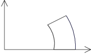
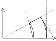
Figure 2: Illustration of over-approximation algorithm of Sec. 4 with Example 2. Left: The set $T_{0}$. Right: Result obtained by the schematic algorithm of Sec. 4, with exact values for $l_{i}$ and $l_{i}^{\prime}$. It may be observed that only $5$ of the $4k=4\times 3=12$ hyperplanes that the the algorithm computes are required for this example, provided that $l_{i}$ and $l_{i}^{\prime}$ can be found exactly.

Now, recalling the notation of Sec. 4, we may take $\delta=1$, $\delta_{0}=\frac{\sqrt{3}}{2}$. It is easy to check that $M_{0}=\sqrt{2}$ and $\|\mathbf{a}_{i}^{T}A\|=\|\mathbf{b}_{i}^{T}A\|=1$, for $1\leq i\leq 3$. Hence

$$l_{i}\leq\hat{l}=\frac{\sqrt{2}\times 1\times e^{\pi/6}}{\sqrt{3}/2}=\frac{2\sqrt{2}\times e^{\pi/6}}{\sqrt{3}}\approx 2.7566424$$

and the same upper bound holds for $l_{i}^{\prime}$, since $\delta_{1}=\delta_{0}$ in this example. For $l_{k}$ and $l_{k}^{\prime}$ we have the following bounds:

$$l_{k}=l_{k}^{\prime}\leq\hat{l}_{k}=\sqrt{2}\times\frac{\pi}{6}\times e^{\pi/6}\approx 1.249999$$

In this example, the same upper bound, given by $\hat{l}_{k}$, holds for $l_{k+i}$ and $l_{k+i}^{\prime}$. Combining all this, the polyhedron is the intersection of the half-spaces given by $\eta_{i}(\mathbf{x})\leq 0$ and $\eta_{i}^{\prime}(\mathbf{x})\leq 0$, $1\leq i\leq 6$, where

$$\eta_{1}(\mathbf{x})=~{}x_{1}-2.7566424\;x_{2}-\sqrt{2}, \eta_{1}^{\prime}(\mathbf{x})=~{}-0.5122958\;x_{1}+2.8873223\;x_{2}-\sqrt{2},$$

$$\eta_{2}(\mathbf{x})=~{}-x_{1}-2.7566424\;x_{2}+1.0, \eta_{2}^{\prime}(\mathbf{x})=~{}-2.2443466\;x_{1}+1.8873223\;x_{2}+1.0,$$

$$\eta_{3}(\mathbf{x})=~{}-x_{2}, \eta_{3}^{\prime}(\mathbf{x})=~{}-x_{1}+\sqrt{3}x_{2},$$

$$\eta_{4}(\mathbf{x})=~{}x_{2}-1.249999, \eta_{4}^{\prime}(\mathbf{x})=~{}0.5\;x_{1}-\frac{\sqrt{3}}{2}x_{2}-1.249999.$$

$$\eta_{5}(\mathbf{x})=~{}x_{1}-\sqrt{2}-1.249999, \eta_{5}^{\prime}(\mathbf{x})=~{}\frac{\sqrt{3}}{2}\,x_{1}+0.5\,x_{2}-\sqrt{2}-1.249999,$$

$$\eta_{6}(\mathbf{x})=~{}-x_{1}+0.249999, \eta_{6}^{\prime}(\mathbf{x})=~{}-\frac{\sqrt{3}}{2}\,x_{1}-0.5\,x_{2}+0.249999.$$

In this example, $\eta_{4}^{\prime}(\mathbf{x})\leq 0$, $\eta_{6}(\mathbf{x})\leq 0$ and $\eta_{6}^{\prime}(\mathbf{x})\leq 0$, are redundant.

Fig. 3 illustrates the result of the algorithm with the first $8$ half-spaces defined by $\eta_{i}(\mathbf{x})\leq 0$ and $\eta_{i}^{\prime}(\mathbf{x})\leq 0$, $1\leq i\leq 4$, where the dashed lines correspond to the lines $\eta_{i}(\mathbf{x})=0$ and $\eta_{i}^{\prime}(\mathbf{x})=0$, and the polyhedron included in their intersection is shown in thick lines. The point of intersection of $\eta_{1}(\mathbf{x})=0$ and $\eta_{4}(\mathbf{x})=0$ is $(4.8600138,\,1.249999)$, of $\eta_{4}(\mathbf{x})=0$ and $\eta_{1}^{\prime}(\mathbf{x})=0$ is $(4.2845099,\,1.249999)$, and of $\eta_{2}(\mathbf{x})=0$ and $\eta_{2}^{\prime}(\mathbf{x})=0$ is $(0.575162,\,0.154114)$. So the vertices in the counter-clockwise order are given by $(\sqrt{2},\,0),\;$ $(4.8600138,\,1.249999),\;$ $(4.2845099,\,1.249999),\;$ $(\sqrt{3}/\sqrt{2},\,1/\sqrt{2}),\;$ $(\sqrt{3}/2,\,0.5),\;$ $(0.575162,\,0.154114)$ and $(1,0)$.

Fig. 4 shows the result when the remaining two half-spaces defined by $\eta_{5}(\mathbf{x})\leq 0$ and $\eta_{5}^{\prime}(\mathbf{x})\leq 0$ are also used. Finally, Fig. 5 shows the intersection of the polyhedron obtained by the method reported in this paper with that which may possibly be obtained by the method of [12], the latter being shown in dotted lines. The polyhedron corresponding to the method of [12] is obtained as follows: the convex hull of the sets $[1,\sqrt{2}]\times\{0\}$ and $\{(a\cos\frac{\pi}{6},a\sin\frac{\pi}{6}):a\in[1,\sqrt{2}]\}$ is the polygon with vertices in the counter-clockwise order $(\sqrt{2},0)$, $({\sqrt{3}}/{\sqrt{2}},1/{\sqrt{2}})$, $({\sqrt{3}}/2,1/{2})$ and $(1,0)$. Therefore the polygon is the interesction of the half-spaces $\zeta_{i}(\mathbf{x})\leq 0$ and $\zeta_{i}^{\prime}(\mathbf{x})\leq 0$, $i=1,2$, where

$$\zeta_{1}(\mathbf{x})=-x_{2}, \zeta_{1}^{\prime}(\mathbf{x})=-x_{1}+\sqrt{3}x_{2},~{}~{}\textrm{ and}$$

$$\zeta_{2}(\mathbf{x})=\frac{1}{\sqrt{2}}(x_{1}-\sqrt{2})-\left(\frac{\sqrt{3}}{\sqrt{2}}-\sqrt{2}\right)x_{2}, \zeta_{2}^{\prime}(\mathbf{x})=-\frac{1}{2}(x_{1}-1)+\left(\frac{\sqrt{3}}{2}-1\right)x_{2}.$$

Now if $\hat{\epsilon}$ is an upper bound for the bloating parameter $\epsilon$, then the half-spaces of the over-approximating polyhedron corresponding to the method of [12] are given by $\hat{\zeta}_{i}(\mathbf{x})\leq 0$ and $\hat{\zeta}_{i}^{\prime}(\mathbf{x})\leq 0$, $i=1,2$, where

$$\hat{\zeta}_{1}(\mathbf{x}) = -x_{2}+\hat{\epsilon},$$

$$\hat{\zeta}_{1}^{\prime}(\mathbf{x}) = -x_{1}+\sqrt{3}x_{2}+\hat{\epsilon},$$

$$\hat{\zeta}_{2}(\mathbf{x}) = 0.70710678x_{1}+0.18946869x_{2}-1+\hat{\epsilon},~{}~{}\textrm{ and}$$

$$\hat{\zeta}_{2}^{\prime}(\mathbf{x}) = -0.70710678x_{1}-0.1339746x_{2}+0.70710678+\hat{\epsilon}$$

The upper bound for the bloating parameter $\epsilon$ as given in [12] works out to be

$$\epsilon \leq M_{0}\left(e^{(\|A\|\Delta)}-1-\|A\|\Delta-\frac{3}{8}\|A\|^{2}\Delta^{2}\right)$$

$$= \sqrt{2}\times\left(e^{(\pi/6)}-1-\frac{\pi}{6}-\frac{3\pi^{2}}{8\times 36}\right)$$

$$= \sqrt{2}\times 0.06168464\approx 0.087235255<0.09.$$

Fig. 5 shows the results when an upper bound for the bloating parameter is chosen to be $\hat{\epsilon}\approx 0.2$, where the dotted lines correspond to the line $\hat{\zeta}_{1}(\mathbf{x})=0$, $\hat{\zeta}_{1}^{\prime}(\mathbf{x})=0$, $\hat{\zeta}_{2}(\mathbf{x})=0$ and $\hat{\zeta}_{2}^{\prime}(\mathbf{x})=0$. As may be expected, the polyhedron of intersection of the two polyhedra – one polyhedron bounded by the dashed lines corresponding to the method described here and another bounded by the dotted lines corresponding to the method of [12] – gives better results of over-approximation.

Figure 3: Illustration of polyhedral over-approximation for the soultion set $T_{0}$ of Example 2: without additional hyperplanes.

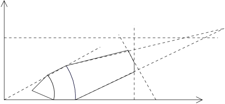
Figure 4: Illustration of polyhedral over-approximation for for the reach set $T_{0}$ of Example 2: with additional hyperplanes.

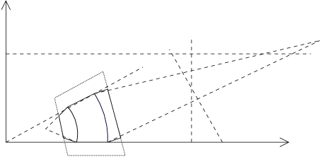
Figure 5: Illustration of polyhedral over-approximation for the solution set $T_{0}$ of Example 2: intersection of the polyhedron that may be obtained by the method of [12] with that obtained by the method reported here.

6 Discussion and Conclusion

An important issue of hybrid systems appears to be computability of the reach sets of the continuous variables. From a computational point, both the problems of computation and efficient representation of the reach sets of the continuous varibles are difficult, in general, owing to the limitations of quantifier elimination method. In this context, approximation of the reach sets by more convenient sets, such as polyhedra and subalgebraic sets, is discussed in the literature. In this paper, along with a method for finding the reach sets, an algorithm for over-approximation of the reach sets with polyhedra when dynamics of the continuous variables are specified by linear differential equations and the inital set is a polyhedron. A practical version of the over-approximation algorithm is also discussed in this paper. However, it seems that better results of over-approximation may be obtained by taking the intersection of the polyhedron obtained by the method reported here with that obtained by the method given in [12]. It is hoped that the over-approximation method presented here may be extended to systems with more general dynamics and initial sets.

Appendix A. Decidable Classes of Subsets of $Q\times\mathbb{R}^{n}$

We introduce here model theoretic concepts for formalizing the notion of decidable class ${\cal C}$ of subsets of $Q\times\mathbb{R}^{n}$ that we were interested in Sec. LABEL:ReachProblems. Since $Q$ is a finite set, for a decidable class ${\cal C}$ of subsets of $Q\times\mathbb{R}^{n}$, we may take, for each $q\in Q$, a decidable class of subsets of $\mathbb{R}^{n}$, ${\cal S}_{q}$, $q\in Q$, and choose ${\cal C}$ to be the product class $\bigcup_{q\in Q}\{\{q\}\times S_{q}:S_{q}\in{\cal S}_{q}\}$. Therefore, we restrict our attention to the discussion of classes of subsets of $\mathbb{R}^{n}$. Most parts of this section are taken from [3] (see also [Laff00], which in turn cites the references [19, 20, 21]).

Definition 11

A language is a tuple of three sets, ${\cal L}=(L_{r},L_{f},L_{c})$, where

1. $L_{r}$ is a set of relations,

2. $L_{f}$ is a set of functions, and

3. $L_{c}$ are a set of constants.

Definition 12

A model of a language ${\cal L}=(L_{r},L_{f},L_{c})$ consists of a nonempty set ${\cal S}$, together with an interpretation of the relations, functions and constants.

We denote a model by $({\cal S},L_{r},L_{f},L_{c})$, where the interpretation is not made explicit. In the following, let ${\cal V}=\{x,y,z,x_{0},x_{2},\ldots\}$ denote a countable set of variables.

Definition 13

A term of a language, ${\cal L}=(L_{r},L_{f},L_{c})$, is inductively defined as follows:

1. each variable $\theta\in{\cal V}$ is a term,

2. each constant $c\in L_{c}$ is a term, and

3. for an $m$-ary function $g\in L_{f}$, where $m\geq 1$, and $m$ terms, $\theta_{1},\theta_{2},\ldots,\theta_{m}$, $g(\theta_{1},\theta_{2},\ldots,\theta_{m})$ is a term.

Definition 14

An atomic formula of a language ${\cal L}$ is either

1. $\theta_{1}=\theta_{2}$, where $\theta_{1}$ are $\theta_{2}$ two terms of ${\cal L}$, or

2. $\rho(\theta_{1},\ldots,\theta_{n})$, where $n\geq 1$ and $\rho\in L_{r}$ is an $n$-ary relation.

Definition 15

A first order formula, or simply a formula, of a language ${\cal L}$ is recursively defined as one of the following:

1. an atomic formula, or

2. $\lnot\phi$, where $\phi$ is formula and $\lnot$ is logical negation, or

3. $\phi_{1}\land\phi_{2}$, where $\phi_{1}$ and $\phi_{2}$ are formulas and $\land$ is logical and, or

4. $\exists x:\phi$ or $\forall x:\phi$, where $\phi$ is a formula, $x$ is a variable, and $\exists$ (there exists) and $\forall$ (for all) are quantifiers; in this case, each occurrence of the variable $x$ in the formula $\phi$ is called a bound occurrence.

Definition 16

The occurrence of a variable in a formula is free, if it is not bound. A sentence in a language ${\cal L}$ is a formula with no free variable. A theory of ${\cal L}$ is a subset of sentences.

For a model ${\cal S}$ of the language ${\cal L}$, we shall be particularly interested in the theory defined by the set of all sentences that are true in ${\cal S}$. To emphasize this, we refer to this theory as the theory of $({\cal S},L_{r},L_{f},L_{c})$.

Definition 17

Let ${\cal L}$ be a language and ${\cal S}$ be a model of ${\cal L}$. A set $X\subset{\cal S}^{n}$ is said to be definable in the language ${\cal L}$, if there is an $n$-ary formula $\phi(x_{1},\ldots,x_{n})$ such that $X$ can be written as $X=\{(x_{1},\ldots,x_{n})\in S^{n}:\phi(x_{1},\ldots,x_{n})\}$.

Definition 18

Let ${\cal L}$ be a language, ${\cal S}$ be a model of ${\cal L}$, and ${\cal C}$ be the class of definable sets. Then ${\cal C}$ is said to be decidable, if the theory of $({\cal S},L_{r},L_{f},L_{c})$ is decidable, i.e., there is a decision procedure that, given an ${\cal L}$-sentence $\phi$, decides whether $\phi$ belongs to the theory of $({\cal S},L_{r},L_{f},L_{c})$ or not.

Examples

1. The theory $(\mathbb{R},\{<\},\{+,-\},\{0,1\})$ is the theory of linear constraints with integer coefficients, denoted by $Lin(\mathbb{R})$. The sets defined by these formulas are called polyhedral sets.

2. The theory $(\mathbb{R},\{<\},\{+,-,\cdot\},\{0,1\})$ is the theory of polynomial constraints with integer coefficients, denoted by $OF(\mathbb{R})$. The sets defined by these formulas are called subalgebraic sets.

The result stated below is due to A. Tarski [22]:

Theorem 1

The first order theory $OF(\mathbb{R})$ is decidable.

Definition 19

Let ${\cal L}$ be a language and let ${\cal S}$ be a model of ${\cal L}$. We say the theory of $({\cal S},L_{r},L_{f},L_{c})$ admits quantifier elimination if every first order formula of $({\cal S},L_{r},L_{f},L_{c})$ is equivalent to a formula of $({\cal S},L_{r},L_{f},L_{c})$ without quantifiers.

Examples: Decidability and Quantifier Elimination

1. The theory $OF(\mathbb{R})$ consisting of $(\mathbb{R},\{<\},\{+,-,\cdot\},\{0,1\})$ admits quantifier elimination and is also decidable.

2. Let $OF_{exp}(\mathbb{R})$ be the theory consisting of $(\mathbb{R},\{<\},\{+,-,\cdot,exp\},\{0,1\})$, where $exp$, representing the exponential function, is a new function symbol. This theory does not admit quantifier elimination, and it is not known whether this theory is decidable. (See [15]).

Appendix B: $Reach_{q}(X_{0},[0,\tau])=X(\tau)=X^{+}(\tau)$

We assume that $X_{0}$ is closed and its boundary, denoted by $S_{0}$, consists of a finite union of smooth surfaces. Let

$$X(\tau)=X_{0}\bigcup_{0\leq t\leq\tau}\{\phi_{q}(\mathbf{x}_{0},t)\hskip 1.42271pt:~{}\mathbf{x}_{0}\in S_{0}\}.$$

Also let

$$S_{0}^{+}=\{\mathbf{x}\in S_{0}\hskip 1.42271pt:\exists\epsilon=\epsilon(\mathbf{x})>0\textrm{ such that }\phi(\mathbf{x},t)\in X_{0}^{c},~{}\forall t\in(0,\epsilon)\},$$ (16)

and $X^{+}(\tau)=X_{0}\bigcup_{0\leq t\leq\tau}\{\phi_{q}(\mathbf{x}_{0},t)\hskip 1.42271pt:~{}\mathbf{x}_{0}\in S_{0}^{+}\}$.

Proposition 1

$X^{+}(\tau)=X(\tau)=Reach(X_{0},[0,\tau])$.

Proof. Note that $X^{+}(\tau)\subset X(\tau)\subset Reach(X_{0},[0,\tau])$. So we have to show that $Reach(X_{0},[0,\tau])\subset X^{+}(\tau)$. Let $\mathbf{z}\in Reach(X_{0},t)$, $t>0$. If $\mathbf{z}\in X_{0}$, then $\mathbf{z}\in X^{+}(\tau)$. Now suppose $\mathbf{z}\not\in X_{0}$. So there is a $\mathbf{z}_{0}\in X_{0}$ such that $\mathbf{z}=\phi(\mathbf{z}_{0},s)$, for some $s$ with $0<s\leq\tau$. If $\mathbf{z}_{0}\in S_{0}^{+}$, then $\mathbf{z}\in X^{+}(\tau)$. Otherwise let $\tau^{\prime}=\sup\{t\hskip 1.42271pt:~{}t\leq s\textrm{ and }\phi(\mathbf{z}_{0},t)\in X_{0}\}$, so $0<\tau^{\prime}<s\leq\tau$. Now $\mathbf{z}^{\prime}=\phi(\mathbf{z}_{0},\tau^{\prime})\in S_{0}^{+}$. Therefore, $\mathbf{z}=\phi(\mathbf{z}^{\prime},s-\tau^{\prime})\in X^{+}(\tau)$.

Now suppose that $X_{0}$ is specified as $X_{0}=\{\mathbf{x}\in\mathbb{R}^{n}:\ell(\mathbf{x})\leq 0\}$, where $\ell:\mathbb{R}^{n}\rightarrow\mathbb{R}$ is continuously differentiable. Further, we assume that if $\mathbf{x}\in{\stackrel{{\scriptstyle\circ}}{{X_{0}}}}$ then $\ell(\mathbf{x})<0$ (where ${\stackrel{{\scriptstyle\circ}}{{X_{0}}}}$ denotes the interior of $X_{0}$, i.e., the largest open set contained in $X_{0}$) So, obviously, if $\mathbf{x}\in S_{0}$ then $\ell(\mathbf{x})=0$, and if $\mathbf{x}\in X_{0}^{c}$ then $\ell(\mathbf{x})>0$. Let $S_{1}^{+}\subset S_{0}$ be defined as

$$S_{1}^{+}=\{\mathbf{x}\in S_{0}\hskip 1.42271pt:~{}\nabla\ell(\mathbf{x})\cdot f(q,\mathbf{x})\geq 0\}.$$

We now show that $S_{0}^{+}\subset S_{1}^{+}$. To this end, we show that $S_{0}\backslash S_{1}^{+}\subset S_{0}\backslash S_{0}^{+}$. Let $\mathbf{x}\in S_{0}\backslash S_{1}^{+}$, so $\nabla\ell(\mathbf{x})\cdot f(q,\mathbf{x})<0$. Now, since $\ell(\phi_{q}(\mathbf{x},0))=\ell(\mathbf{x})=0$, and since at $t=0$, $\frac{d\ell(\phi_{q}(\mathbf{x},t))}{dt}=\nabla\ell(\mathbf{x})\cdot f(q,\mathbf{x})<0$, we have, for a sufficiently small $\epsilon>0$, $\ell(\phi_{q}(\mathbf{x},t))<0$, whenever $0<t<\epsilon$, which happens only if $\phi_{q}(\mathbf{x},t)\in{\stackrel{{\scriptstyle\circ}}{{X_{0}}}}$, $\forall t\in(0,\epsilon)$, implying that $\mathbf{x}\not\in S_{0}^{+}$; hence $\mathbf{x}\in S_{0}\backslash S_{0}^{+}$. Thus $S_{0}\backslash S_{1}^{+}\subset S_{0}\backslash S_{0}^{+}$, as required.

Appendix C: $Reach_{q}^{\prime}\left(X_{0},X_{q},[0,\infty)\right)$

Let $X_{q}\subset\mathbb{R}^{n}$ with compact closure, and let $Y_{q}=\overline{X_{q}}$. Let $\mathbf{f}:W\rightarrow\mathbb{R}^{n}$ be a continuous function defined on an open set $W$ containing $Y_{q}$, satisfying a Lipschitz condition on $W$. Let $X_{0}$ be a closed subset of $Y_{q}$. We assume that for each $\mathbf{x}\in X_{0}$, a function $\gamma_{\mathbf{x}}:\mathbb{R}^{+}\rightarrow\mathbb{R}^{n}$ exists and satisfies the differential equation

$$\frac{d\gamma_{\mathbf{x}}(t)}{dt}=\mathbf{f}(\gamma_{\mathbf{x}}),~{}~{}t\geq 0,$$ (17)

with the initial condition $\gamma_{\mathbf{x}}(0)=\mathbf{x}$. Hence the flow $\phi(\mathbf{x},t)$ associated with equation (17) is defined for all $t\geq 0$ and $\mathbf{x}\in X_{0}$. Further, assume that the $\omega$-limit set of the flow $\phi(\mathbf{x},t)$, $t\geq 0$, does not intersect $Y_{q}$ for any point $\mathbf{x}\in X_{0}$. More precisely, we assume, for $\mathbf{x}\in X_{0}$,

$$L_{\omega}(\mathbf{x})\bigcap Y_{q}=\emptyset,$$ (18)

where

$$L_{\omega}(\mathbf{x})=\bigcap_{t\geq 0}\overline{\phi(\mathbf{x},[t,\infty))}.$$

(See [16, 17].) In what follows, we show that if (18) holds for every $\mathbf{x}\in X_{0}$, then $\exists\tau_{\max}>0$ (depending on $X_{0}$), such that for every $\mathbf{x}\in X_{0}$, there is a $\tau=\tau(\mathbf{x})$ with $0<\tau(\mathbf{x})\leq\tau_{max}$ and $\phi(\mathbf{x},t(\mathbf{x}))\not\in Y_{q}$. For this, let $0<\tau_{1}<\tau_{2}<\ldots$ be an increasing sequence such that $\tau_{k}\rightarrow\infty$, as $k\rightarrow\infty$ (as in Sec. 3), and define the sets $A(\tau_{k},\mathbf{x})=\overline{\phi(\mathbf{x},[\tau_{k},\infty))}$. We first observe that $L_{\omega}(\mathbf{x})=\bigcap_{k}A(\tau_{k},\mathbf{x})$.

Proposition 2

Let $\mathbf{x}\in X_{0}$. If (18) holds, then $\exists\tau=\tau(\mathbf{x})>0$ such that $\phi(\mathbf{x},t)\not\in Y_{q}$, $\forall t\geq\tau$.

Proof. We have $L_{\omega}(\mathbf{x})\bigcap Y_{q}=$ $\left[\bigcap_{k}A(\tau_{k},\mathbf{x})\right]\bigcap Y_{q}$ $=\bigcap_{k}\left[A(\tau_{k},\mathbf{x})\bigcap Y_{q}\right]$. Now let $E(\tau_{k},\mathbf{x})=A(\tau_{k},\mathbf{x})\bigcap Y_{q}$. So, for a fixed $\mathbf{x}\in X_{0}$, the sets $E(\tau_{k},\mathbf{x})$, $k=1,2,3,\ldots$, is a decreasing sequence of closed subsets of $Y_{q}$. Since $Y_{q}$ is compact, $\bigcap_{k}E(\tau_{k},\mathbf{x})=\emptyset$ implies $E(\tau_{k},\mathbf{x})=\emptyset$, for all but finitely many $k$. Therefore, for some $K\geq 1$, $\forall k\geq K$, $E(\tau_{k},\mathbf{x})=\emptyset$. Hence, $\phi(\mathbf{x},[t,\infty))\bigcap Y_{q}=\emptyset$, $\forall t\geq\tau_{K}$. Therefore, with $\tau=\tau_{K}$, $\phi(\mathbf{x},t)\not\in Y_{q}$, $\forall t\geq\tau$.

We also need the following proposition:

Proposition 3

Let $\mathbf{x}\in X_{0}$ be a point for which there is a $\tau>0$, such that $\phi(\mathbf{x},\tau)\not\in Y_{q}$. Then there is a $\delta=\delta_{\mathbf{x}}>0$, such that if $|\mathbf{x}-\mathbf{y}|<\delta_{\mathbf{x}}$ and $\mathbf{y}\in X_{0}$, then $\phi(\mathbf{y},\tau)\not\in Y_{q}$.

Proof. Let $|\mathbf{f}(\mathbf{x})-\mathbf{f}(\mathbf{y})|\leq C|\mathbf{x}-\mathbf{y}|$. Then $|\phi(\mathbf{x},\tau)-\phi(\mathbf{y},\tau)|\leq|\mathbf{x}-\mathbf{y}|e^{\hskip 1.42271ptC\tau}$ (see, for example, [17]), so for a fixed $\tau$, $\phi(\cdot,\tau)$ is continuous in the first variable. Let $\mathbf{z}=\phi(\mathbf{x},\tau)$. Now since $W\backslash Y_{q}$ is open, there is an $\epsilon>0$ such that $B(\mathbf{z},\epsilon)\subset W\backslash Y_{q}$. By the continuity of $\phi(\cdot,\tau)$ at $\mathbf{x}$, there is a $\delta>0$, such that $|\phi(\mathbf{x},\tau)-\phi(\mathbf{y},\tau)|=|\mathbf{z}-\phi(\mathbf{y},\tau)|<\epsilon$, whenever $|\mathbf{y}-\mathbf{x}|<\delta$ and $\mathbf{y}\in X_{0}$. Therefore, $\phi(\mathbf{y},\tau)\in B(\mathbf{z},\epsilon)\subset W\backslash Y_{q}$.

From the previous two propositions, we get the following theorem:

Theorem 2

Let $Y_{q}$ be compact, and $\mathbf{f}$ be a continuous function defined on an open set $W$ containing $Y_{q}$ satisfying a Lipschitz condition. Further assume condition (18) holds for every $\mathbf{x}\in X_{0}$. Then $\exists\tau_{\max}>0$ independent of $\mathbf{x}$, such that for each $\mathbf{x}\in X_{0}$, there is a $\tau(\mathbf{x})$ with $0<\tau(\mathbf{x})\leq\tau_{max}$ and $\phi(\mathbf{x},\tau(\mathbf{x}))\not\in Y_{q}$.

Proof. Let $\mathbf{x}\in X_{0}$. By Proposition 2, there is a $\tau(\mathbf{x})>0$, such that $\phi(\mathbf{x},\tau(\mathbf{x}))\not\in Y_{q}$. By Proposition 3, there is a $\delta_{\mathbf{x}}>0$, such that for any $\mathbf{y}\in X_{0}$ with $|\mathbf{y}-\mathbf{x}|<\delta_{\mathbf{x}}$, $\phi(\mathbf{y},\tau(\mathbf{x}))\not\in Y_{q}$. $\{B(\mathbf{x},\delta_{\mathbf{x}})\hskip 1.42271pt:\mathbf{x}\in X_{0}\}$ is an open cover of $X_{0}$, containing a finite subcover, say, $\{B(\mathbf{x}_{1},\delta_{\mathbf{x}_{1}}),\ldots,B(\mathbf{x}_{m},\delta_{\mathbf{x}_{m}})\}$. Let $\tau_{\max}=\max\{\tau(\mathbf{x}_{1}),\ldots,\tau(\mathbf{x}_{m})\}$. To check wether this choice of $\tau_{max}$ is as in the theorem, let $\mathbf{y}\in X_{0}$ be an arbitrary point. Now $\mathbf{y}\in B(\mathbf{x}_{i},\delta_{\mathbf{x}_{i}})$, for some $i$ with $1\leq i\leq m$, and by the choice of $\delta_{\mathbf{x}_{i}}$, $\phi(\mathbf{y},\tau(\mathbf{x}_{i}))\not\in Y_{q}$, concluding the proof.

Appendix D: Boundedness Results

In this section, we show that if the initial set $F$ is bounded then the polyhedron, $P$, enclosing $F_{[0,\Delta]}$, as obtained by the algorithm described in Sec. 3 is bounded. We assume that $F$ is nonempty. Recall that $F$ is given as the set of points $\mathbf{x}$ in $\mathbb{R}^{n}$ which satisfy the following constraints:

$$\left.\begin{array}[]{rcl}\mathbf{a}_{i}^{T}\mathbf{x}-b_{i}&\leq&0,~{}~{}i=1,2,\ldots,k-1,\\ \mathbf{a}_{k}^{T}\mathbf{x}-b_{k}&=&0,\end{array}\right\}$$ (19)

and $P$ is included in the set of points $\mathbf{x}\in\mathbb{R}^{n}$ satisfying

$$\left.\begin{array}[]{rcl}\mathbf{a}_{i}^{T}\mathbf{x}-b_{i}-l_{i}(\mathbf{a}_{k}^{T}\mathbf{x}-b_{k})&\leq&0,~{}~{}i=1,2,\ldots,k-1,\\ \mathbf{a}_{k}^{T}\mathbf{x}-b_{k}&\geq&0,~{}~{}\textrm{ and}\\ \mathbf{a}_{k}^{T}\mathbf{x}-b_{k}-l_{k}&\leq&0,\end{array}\right\}$$ (20)

where $l_{i}\in\mathbb{R}$ and $l_{k}>0$. Looking at the constraints, one may visualize the set $P_{1}$ satisfying (20) as a prism or a truncated pyramid, with its bottom given by (19) and its top given by

$$\left.\begin{array}[]{rcl}\mathbf{a}_{i}^{T}\mathbf{x}-b_{i}-l_{i}(\mathbf{a}_{k}^{T}\mathbf{x}-b_{k})&\leq&0,~{}~{}i=1,2,\ldots,k-1,\\ \mathbf{a}_{k}^{T}\mathbf{x}-b_{k}-l_{k}&=&0.\end{array}\right\}$$ (21)

We assume that $F$ is nonempty, and wish to show that if $F$ is bounded then so is the set $P_{1}$, defined as the set of points satisfying (20). We start with the following proposition:

Proposition 4

Assume that $F$ is nonempty and $P_{1}$ is not bounded. Then there is a point $\mathbf{x}_{0}\in F$ and a vector $\lambda\in\mathbb{R}^{n}$, with $|\lambda|=1$, such that $\mathbf{x}_{0}+t\lambda\in P_{1}$, for all $t\geq 0$.

Proof. Fix a point $\mathbf{x}_{0}\in F$, and suppose $P_{1}$ is not bounded. So for each positive integer $k$, there is a point $\mathbf{x}_{k}\in P_{1}$, such that $|\mathbf{x}_{k}-\mathbf{x}_{0}|\geq k$. Let $\lambda_{k}=\frac{(\mathbf{x}_{k}-\mathbf{x}_{0})}{|\mathbf{x}_{k}-\mathbf{x}_{0}|}$. Now, since $F\subset P_{1}$, $\mathbf{x}_{0}\in P_{1}$ and, by convexity, the entire line segment $\mathbf{x}_{0}+t\lambda_{k}\in P_{1}$, for $0\leq t\leq k$. In particular, the points on these line segments satisfy (20). Now, since for each $k$, $|\lambda_{k}|=1$, and the closed unit ball in $\mathbb{R}^{n}$ is compact, there is a convergent subsequence of $\lambda_{k}$’s – say, $\lambda_{k_{i}}$, $i=1,2,3,\ldots$ – such that $\lambda_{k_{i}}\rightarrow\lambda\in\mathbb{R}^{n}$, as $i\rightarrow\infty$; since $|\lambda_{k_{i}}|=1$, $|\lambda|=1$. We show that $\mathbf{x}_{0}+t\lambda\in P_{1}$ for $t\in[0,\infty)$. First note that for any positive integer $m$, and for all $i\geq m$, $\mathbf{x}_{0}+t\lambda_{k_{i}}$ satisfies the constraints (20), for $t\in[0,k_{m}]$. Therefore, $\mathbf{x}_{0}+t\lambda$ satisfies (20), for $t\in[0,k_{m}]$, and so $\mathbf{x}_{0}+t\lambda\in P_{1}$, for $t\in[0,k_{m}]$. The proposition is concluded by letting $m\rightarrow\infty$.

We now show that such an $\lambda$, as in the previous proposition, must be parallel to the hyperplane passing through $F$, the normal of which is given by $\mathbf{a}_{k}$.

Proposition 5

If $\mathbf{x}_{0}\in F$ and a unit vector $\lambda\in\mathbb{R}^{n}$ are such that $\mathbf{x}_{0}+t\lambda\in P_{1}$, for all $t\in[0,\infty)$, then $\mathbf{a}_{k}^{T}\lambda=0$.

Proof. For a contradiction assume that $h=\mathbf{a}_{k}^{T}\lambda>0$. Now since $\mathbf{x}+t\lambda$ satisfies (20), we must have

$$\mathbf{a}_{k}^{T}(\mathbf{x}_{0}+t\lambda)-b_{k}-l_{k}\leq 0,$$

which holds only if $t\leq\frac{(b_{k}+l_{k}-\mathbf{a}_{k}^{T}\mathbf{x}_{0})}{h}$, contrary to the hypothesis that, for all $t\in[0,\infty)$, $\mathbf{x}_{0}+t\lambda\in P_{1}$. Similarly, if $h=\mathbf{a}_{k}^{T}\lambda<0$, then the constraint

$$\mathbf{a}_{k}^{T}(\mathbf{x}_{0}+t\lambda)-b_{k}\geq 0,$$

does not hold for $t>0$. Therefore we must have $\mathbf{a}_{k}^{T}\lambda=0$.

We now show that if $F$ is bounded, then for any unit vector $\lambda$ orthogonal to $\mathbf{a}_{k}$, there is an $i$ with $1\leq i\leq k-1$, such that $h_{i}=\mathbf{a}_{i}^{T}\lambda>0$.

Proposition 6

If $F$ is nonempty and bounded, then for any unit vector $\lambda\in\mathbb{R}^{n}$, for which $\mathbf{a}_{k}^{T}\lambda=0$, there is an $i$, with $1\leq i\leq k-1$, such that $\mathbf{a}_{i}^{T}\lambda>0$.

Proof. Let $\mathbf{x}_{0}\in F$, and suppose that there is an $\lambda\in\mathbb{R}^{n}$, with $|\lambda|=1$, $\mathbf{a}_{k}^{T}\lambda=0$ and $\mathbf{a}_{i}^{T}\lambda\leq 0$, for $1\leq i\leq k-1$. Then for any $t>0$, the vector $\mathbf{x}_{0}+t\lambda$ satisfies the constraints (19), and so $\mathbf{x}_{0}+t\lambda\in F$, contrary to the assumption that $F$ is bounded.

We now combine all the previous propositions to get the following result:

Theorem 3

If $F$ is nonempty and bounded, then $P_{1}$ is bounded.

Proof. If $P_{1}$ is not bounded, then by Proposition 4, there is an $\mathbf{x}_{0}\in F$ and a unit vector $\lambda\in\mathbb{R}^{n}$ such that $\mathbf{x}_{0}+t\lambda\in P_{1}$, for any $t\geq 0$. By Proposition 5, $\mathbf{a}_{k}^{T}\lambda=0$. Now, by the previous proposition, since $F$ is bounded, there is an $i$, with $1\leq i\leq k-1$, such that $h_{i}=\mathbf{a}_{i}^{T}\lambda>0$. But then the constraint

$$\mathbf{a}_{i}^{T}(\mathbf{x}_{0}+t\lambda)-b_{i}-l_{i}(\mathbf{a}_{k}^{T}(\mathbf{x}_{0}+t\lambda)-b_{k})\leq 0,$$

cannot hold for any $t$ with

$$t>-\frac{\mathbf{a}_{i}^{T}\mathbf{x}_{0}-b_{i}}{h_{i}},$$

contrary to the assumption that $\mathbf{x}_{0}+t\lambda\in P_{1}$, for any $t\geq 0$. Hence $P_{1}$ is bounded.

References

- [1] R. Alur, C. Courcoubetis, N. Halbwachs, T. A. Henzinger, P.-H. Ho, X. Nicollin, A. Olivero, J. Sifakis and S. Yovine, “The algorithmic analysis of hybrid systems”, Theoretical Computer Science, Vol 138, pp. 3-35, 1995.
- [2] Y. Kesten, A. Pnueli, J. Sifakis, and S. Yovine, “Decidable Integration Graphs”, Information and Computation, Vol. 150, No. 2, p. 209 - 243, 1999.
- [3] G. Lafferriere, G. J. Pappas and S. Yovine, “A New Class of Decidable Hybrid Systems”, Lecture Notes in Computer Science, Vol. 1569, pp. 137-151, 1999.
- [4] G. Lafferriere, G. J. Pappas and S. Yovine, “Reachability Computation of Linear Hybrid Systems” Proc. 14th IFAC World Congress, Vol. E, pp. 7-12, Beijing, PRC, July 1999.
- [5] T. A. Henzinger, P.-H. Ho, and H. Wong-Toi, “Algorithmic analysis of nonlinear hybrid systems”, IEEE Trans. Automatic Control, Vol. 43, pp. 540-554, 1998.
- [6] O. George J. Pappas, S. Sastry, “Semidecidable Controller Synthesis for Classes of Linear Hybrid Systems”, Proc. 39th IEEE Conf. on Decision and Control, Sydney, Australia, Dec. 2000
- [7] E. Asarin, O. Bournez, T. Dang, O. Maler, A. Pnueli, “Effective Synthesis of Switching Controllers for Linear Systems”, Proceedings of the IEEE, Vol. 88, No. 7, pp. 1011-1025, 2000.
- [8] T. Dang and O. Maler, “Reachability analysis via face lifting”, T. A. Henzinger and S. Sastry (Eds.) Hybrid Systems: Computation and Control, LNCS 1386, pp. 96-109, Springer Verlag, New York, 1998.
- [9] C. Tomlin, J. Lygeros, and S. Sastry, “Synthesizing controllers for nonlinear hybrid systems”, in Hybrid Systems: Computation and Control, LNCS 1386, pp. 360–373, Springer Verlag, New York, 1998.
- [10] P. Varaiya, “Reach set computation using optimal control”, Proc. KIT Workshop, Verimag, Grenoble, 1998.
- [11] A. B. Kurzhanski and P. Varaiya, “Ellipsoidal techniques for reachability analysis: internal approximation”, Systems & Control Letters, Vol. 41, No. 3, Oct. 2000.
- [12] E. Asarin, O. Bournez, T. Dang, and O. Maler, “Approximate reachability analysis of piece-wise linear dynamical systems”, in Hybrid Systems: Computation and Control, March 2000, Pittsburgh, USA.
- [13] O. Maler, A. Pnueli and J. Safakis, “On the Synthesis of Discrete Controllers for Timed Systems (An Extended Abstract)”, Proc. STACS ’95, LNCS 900, pp. 229-242, Springer, 1995.
- [14] T. A. Henzinger, “Hybrid automata with finite bisimulations”, Proc. ICALP ’95, LNCS 944, pp. 324-33 Springer-Verlag, 1995.
- [15] G. J. Pappas, “Hybrid Systems: Computation and Abstraction”, Ph.D. Thesis, Electrical Engineering and Computer Sciences, University of California at Berkeley.
- [16] J. H. Hubbard and B. H. West, “Differential equations: a dynamical systems approach”, Springer-Verlag, New York, 1995.
- [17] M. W. Hirsch and S. Smale, “Differential Equations, Dynamical Systems and Linear Algebra”, Academic Press, New York, 1974.
- [18] R. T. Rockafellar, “Convex Analysis”, Princeton University Press, Princeton, New Jersey, 1970.
- [19] W. Hodges, “A Shorter Model Theory”, Cambridge University Press, 1997.
- [20] D. Marker, “Model Theory and Exponentiation”, Notices of AMS, Vol. 43, No. 7, pp. 753-759, 1996.
- [21] D. van Dalen, “Logic and Structure”, Springer-Verlag, Third Edition, 1994.
- [22] A. Tarski, “A Decision Method for Elementary Algebra and Geometry”, University of California Press, Second Edition, 1951.
- [23] L. van Den Dries, “Remarks on Tarski’s problem concerning ”, in G. Lolli, G. Longo and A. Marcja, editors, Logic Colloquium ’82, pp. 97-121, Elsevier Science Publishers B.V., 1984.