A Qualitative Dynamical Modelling Approach to Capital Accumulation in Unregulated Fisheries

Abstract

Capital accumulation has been a major issue in fisheries economics over the last two decades, whereby the interaction of the fish and capital stocks were of particular interest. Because bio-economic systems are intrinsically complex, previous efforts in this field have relied on a variety of simplifying assumptions. The model presented here relaxes some of these simplifications. Problems of tractability are surmounted by using the methodology of qualitative differential equations (QDE). The theory of QDEs takes into account that scientific knowledge about particular fisheries is usually limited, and facilitates an analysis of the global dynamics of systems with more than two ordinary differential equations. The model is able to trace the evolution of capital and fish stock in good agreement with observed patterns, and shows that over-capitalization is unavoidable in unregulated fisheries.

1 Introduction

Following sustained interest from policy makers, recent years have seen a number of bio-economic models examining the effects of commercial fisheries on marine resources. Even though over-fishing has been a fact since historical times (Jackson et al., 2001), the problem has gained a new quality due to the industrialization of fisheries (Fao, 2004). In particular the latter has reduced fish biomass by 80% within 15 years of exploitation (Myers and Worm, 2003). In this context, the impact of capital accumulation has been a major issue in fisheries economics over the last two decades (Clark et al., 1979; McKelvey, 1985; Boyce, 1995; Jørgensen and Kort, 1997; Munro, 1999; Pauly et al., 2002). In these contributions, commercial fisheries is portrayed as a system in which a biological stock and a capital stock interact dynamically. As the capital stock is highly specialized and cannot readily be converted to other uses, investment decisions are characterized by irreversibility, which is assumed as a major cause of over-fishing.

The previous literature has treated capital accumulation in various settings. Clark et al. (1979) study the optimal management strategy for a renewable resource with irreversible investment, assuming that marginal investment costs are constant. The latter assumption is abandoned by Boyce (1995) on the grounds that constant investment costs imply an immediate jump in the capital stock, which is then followed by a period of decline in both the capital and fish stock. Contrary, observed patterns of capital accumulation are characterized by an initial phase of continuous growth of fleet size. Assuming increasing marginal investment costs leads to better agreement with observations, but makes the model more complicated. Considerations of tractability therefore lead Boyce (1995) to assume that harvest productivity is independent of the size of the biological stock.

In contrast to these optimal-exploitation models, approaches which study capital accumulation in more realistic settings are rare. An exception is McKelvey (1985, 1986) who examines an open-access fishery with irreversible investment under both perfect and imperfect competition. But the increased realism of these models comes at a cost in that marginal investment costs and harvesting productivity are kept constant in the analysis of out-of-equilibrium behaviour due to serious analytical difficulties. In general, the variety of modelling strategies pursued in the literature thus reflects the tension between realism and tractability, illustrating the need for new concepts in integrated modelling (cf. Knowler, 2002; Müller, 2003). In order to keep them accessible to analysis, most of the models mentioned above disregard at least one of these difficulties, e.g. those relating to investment costs, harvesting productivity, or industry structure. In many cases the difficulties restrict analysis to equilibria or comparative dynamics in the neighbourhood of an equilibrium. But since fisheries systems tend to stay far away from equilibrium, e.g. when catches reside above the maximum sustainable yield, there exists an urgent need for the analysis of the enfolding dynamics. A common approach to this task is phase plane analysis. Although this technique is not impossible for systems with more than two ordinary differential equations (ODEs), it becomes rather difficult (cf. Berck and Perloff, 1984). Another technique to tackle tractability problems might be to run an ensemble of numerical simulations or to use methods from nonlinear analysis (e.g. bifurcation analysis or computing domains of attraction) rather than solving analytical models. These approaches are limited if precise parameters and exact functional specifications are not completely available. In fact, as pointed out by Clark (1999), our understanding of bio-economic systems is characterized by low levels of knowledge. The dynamics of fish stocks, the economic characteristics and strategies of the fishing industry are subject to a serious lack of information (cf. Pindyck, 1984; Charles, 2001).

In this paper we demonstrate a qualitative simulation technique which complements phase space analysis and numerical simulation in data-poor settings when nonlinear dynamics far from equilibrium are to be investigated. The method, developed in the field of artifical intelligence (c.f. de Kleer and Brown, 1984; Forbus, 1990; Kuipers, 1994), starts from the argument that imprecise understanding can be formalized and used for a variety of model-based tasks (e.g. identification of general dynamic properties, scenario testing, hypothesis exploration, policy advice). The approach allows all possible dynamic behaviours of the system to be characterized and classified on the basis of purely qualitative relationships (i.e. in the absence of quantitative information). It is used to an increasing extent in several fields (Farley and Lin, 1990; Benaroch and Dhar, 1995, economics and finance), (Heidtke and Schulze-Kremer, 1998; Trelease et al., 1999, epidemiology and genetics), (Juniora and Martin, 2000, chemistry), (Guerrin and Dumas, 2001; Bredeweg and Salles, 2003, ecology), (Eisenack and Kropp, 2001; Petschel-Held and Lüdeke, 2001; Kropp et al., 2002; Schellnhuber et al., 2002, sustainability science), but seldom in bio-economics so far.

We use qualitative simulation to investigate the dynamics of capital accumulation in unregulated fisheries with nonlinear investment costs and stock-dependent harvesting productivity. Our model is able to trace the evolution of capital and fish stocks in good agreement with observed patterns. A main result is that the model necessarily produces a period where the capital stock continues to rise even after the harvest has started to decline, i.e. the development of excess capacities is unavoidable. In general the paper shows that qualitative models allow us to derive robust properties of bio-economic systems when we have only weak knowledge at hand.

We have organized this paper as follows: in section 2 the basics of qualitative modelling are introduced. Section 3 develops an analytical model of capital accumulation in fisheries. In section 4 we generalize this model to a qualitative one to characterize its global dynamic features. In section 5 we compare the results with some development paths recently observed in industrial fishery and draw general implications for fisheries management and the applicability of the QDE method. A discussion and a summary conclude the paper.

2 Foundations of Dynamical Qualitative Modelling

Qualitative differential equations (QDEs) are a prominent methodology in qualitative modelling. For this goal Kuipers (1994) has developed the QSIM runtime environment whose underlying concept is used for the analyses presented here. In the following we describe the basic ideas of QDEs and provide the necessary technical terms (written in italics). For a more detailed introduction and a thorough overview of applications we refer to Kuipers (1994). The input for a modelling task is a qualitative differential equation (QDE) comprising the following parts:

1. a set of continuously differentiable functions (variables) of time;

2. a quantity space for each variable, specified in terms of an ordered set of symbolic landmarks;

3. a set of constraints expressing the algebraic, differential or monotonic relationships between the variables.

A QDE can be considered as an abstract description (abstraction, cf. Fig. 1) of a set of ordinary differential equations (ODEs). The abstraction is attained in a twofold manner: (i) variables take values from the set of symbolic landmarks or intervals between landmarks. Each landmark represents a real number, e.g. maximum sustainable yield, of which the exact quantitative value may be unknown. Nevertheless, it is analytically distinguished whether the catch is above or below this threshold. The landmark or the interval between landmarks where the value of a variable is at a given time, is called its qualitative magnitude. (ii) Monotonic relationships specified between variables, e.g. that the yield is monotonically decreasing with a decreasing stock, are expressed by constraints. This is an abstraction in the sense that the constraint comprises an entire family of (linear and nonlinear) monotonic functions. The only requirement is that these functions are smooth and that their derivatives have certain signs. Qualitative simulation achieves its result by performing a constraint satisfaction scheme (for a general introduction see Tsang, 1993; Dechter, 2003), where all combinations of qualitative magnitudes inconsistent with the constraints are filtered out. Due to continuity of the variables’ values in time, the scheme additionally checks which admissible combinations of qualitative magnitudes can occur after other combinations, called successors. The guaranteed coverage theorem (an in-depth discussion of this theorem is beyond the scope of this paper, see Kuipers, 1994, p.118) ensures that the algorithm predicts an abstract description of all solutions to any ODE described by the given QDE. This implies, due to the indeterminacy of analysed systems, that a QDE solution comprises not only one time development, but a set of trajectories.

In the following we illustrate these concepts considering a simple nonlinear model, which is not meant to solve real-world problems (it will be extended in the succeeding sections).

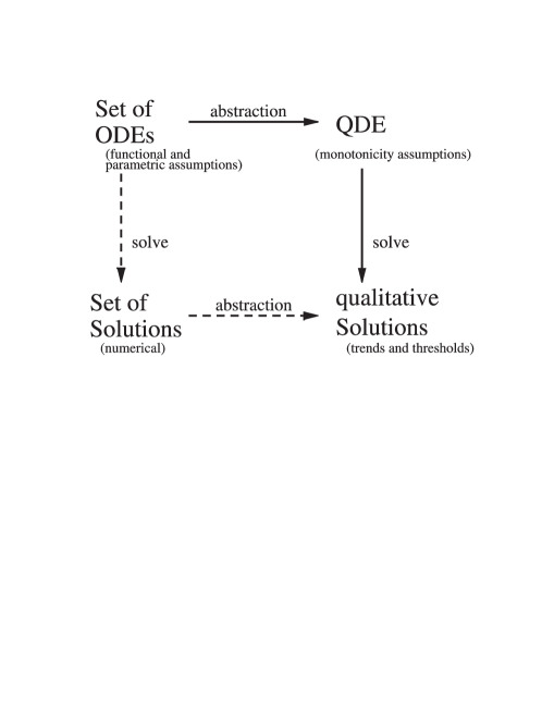
Figure 1: Relationships between ordinary (ODE) and qualitative differential equations (QDE). A reasoning process indicated by the dashed arrows is infeasible if we want to achieve all numerical solutions. This becomes possible by qualitative simulation (solid arrows) since this allows a complete computation of systems development.

Consider a natural resource stock $x$ with an associated recruitment function $R(x)$. The industry chooses effort depending on $x$ such that there is a harvest function $h(x)$. The time behaviour of the stock is expressed as

$$\dot{x}=R(x)-h(x).$$ (1)

It is assumed that $h(0)=0$, and that $h$ is strictly increasing in $x$. The recruitment function is of logistic type and attains a maximum $MSY$ (maximum sustainable yield) at $x_{MSY}$. Furthermore, $R(0)=R(Q)=0$, where $Q$ denotes the carrying capacity of the biological system. For $x<x_{MSY}$ the function $R$ is strictly increasing, but strictly decreasing if $x>x_{MSY}$. In the first abstraction step, for each variable the following sets of symbolic landmarks are defined (including lower and upper bounds):

$$x: \quad 0\quad< \quad x_{MSY}\quad< \quad Q\quad< x_{max},$$

$$h: \quad 0\quad< \quad MSY \quad<\quad h_{max},$$ (2)

$$R: \quad 0\quad< \quad R_{MSY} \quad<\quad R_{max}.$$

For a given time $t$ and a (continuous) value for $x(t)$, $h(t)$ and $R(t)$ one can determine the qualitative magnitudes with respect to the defined landmarks, e.g. as an interval $h(t)\in(MSY,h_{max})$, if $h>MSY$, or as a singular landmark, e.g. $h(t)=MSY$. Qualitative simulation explicitly tracks the direction of change of all variables in the model, which is called qualitative direction. The arrow $\downarrow$ portrays that a variable is decreasing (i.e. $\dot{x}(t)<0$), $\uparrow$ increasing ($\dot{x}(t)>0$), and a circle $\circ$ that $\dot{x}(t)=0$ at a given time $t$. The qualitative magnitude together with the qualitative direction of a variable at a given time is called its qualitative value, e.g. written as $\big{<}(MSY,h_{max}),\uparrow\big{>}$. The qualitative values of all variables of the model calculated for a certain time is called the qualitative state of the system.

In the second abstraction step the constraints of the naïve model are formulated as relationships between the variables and their derivatives. To simplify the presentation we only introduce the most important constraints of the model (for the whole model we refer to the annex and to the download version; cf. footnote 2).

Since $h_{x}>0$, $\dot{h}=h_{x}(x)\cdot\dot{x}$ and $h(0)=0$, using the the sign operator $sgn(\cdot)$,

$$sgn(\dot{h})=sgn(\dot{x})\qquad\text{and}\qquad x=0\Leftrightarrow h=0.\\$$ (3)

We define $R_{MSY}:=R(x_{MSY})$ and describe the relation between stock and recruitment by the monotonicity assumptions mentioned above by:

if $$x=0\quad R=0,$$ then (4)

$$x=x_{MSY} R=R_{MSY},$$ if, and only if (5)

if $$x=Q\quad R=0,$$ then (6)

if $$x<x_{MSY}\quad sgn(\dot{R})=sgn(\dot{x})\quad \text{and}\quad R<R_{MSY},$$ then (7)

if $$x=x_{MSY}\quad \dot{R}=0\quad \text{and}\quad R=R_{MSY},$$ then (8)

if $$x>x_{MSY}\quad sgn(\dot{R})=-sgn(\dot{x})\quad \text{and}\quad R<R_{MSY}.$$ then (9)

The relation $\dot{x}=R-h$ implies

if $$R<R_{MSY} \text{and}\quad h>MSY \dot{x}<0,$$ then (10)

indicating that a recruitment below and a harvest above a sustainable level leads to a decreasing stock. It is obvious, due to the indeterminacy of the relations, that many functions exist which comply with these constraints (see, e.g. Fig. 2a), but nonetheless a complete qualitative simulation is possible.

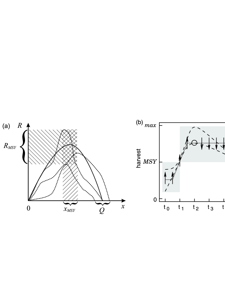
Figure 2: (a) Representation of imprecise knowledge in a QDE model. Shown are some possible realizations of recruitment functions (dashed lines) satisfying the constraints (4)–(9). The uncertainty intervals regarding the landmarks are indicated by brackets. For $R(x_{MSY})$ all values are possible lying in the cross-hatched area. (b) An example for the qualitative behaviour of harvest $h(t)$ (dotted line). Such a behaviour is representative for a class of (quantitative) time developments as indicated by the dashed lines (grey areas).

It starts with a qualitative state as initial value at time $t_{0}$. Supposing that at the beginning the fishery is characterized by an almost unexploited biological stock and catches above $MSY$, the qualitative state at $t_{0}$ is given by

$$x(t_{0})=\big{<}(x_{MSY},Q),\downarrow\big{>},h(t_{0})=\big{<}(MSY,h_{max}),\downarrow\big{>},R(t_{0})=\big{<}(0,R_{MSY}),\uparrow\big{>}.$$ (11)

The qualitative magnitude of $R$ results from the qualitative magnitude of $x$ (above $x_{MSY}$) by applying constraint (9). The qualitative direction of $x$ (decreasing) is a consequence of the qualitative magnitudes of $h$ and $R$, i.e. rule (10). Constraint (9) forces $R$ to increase. Finally, $h$ decreases due to constraint (3). A time evolution is now initiated by these starting conditions, which has to respect the direction of changes shown in Eqs. (11) and the defined constraints. For the example three possible evolutions can be distinguished:

1. $x$ decreases below $x_{MSY}$, where $h$ still resides above $MSY$ at this time.

2. $h$ decreases below $MSY$, while $x$ stays above $x_{MSY}$ at this time.

3. $x$ decreases below $x_{MSY}$ and $h$ decreases below $MSY$ at the same time.

These ‘events’ (occurring at a time $t_{1}>t_{0}$) lead to new (and different) qualitative states. Qualitative simulation checks which of these states comply with all constraints of a defined QDE. Those states ‘surviving’ this test are the successors valid for the next time interval. For case (i), we obtain the following qualitative state as a successor:

$$x(t_{1},t_{2})=\big{<}(0,x_{MSY}),\downarrow\big{>},h(t_{1},t_{2})=\big{<}(MSY,h_{max}),\downarrow\big{>},R(t_{1},t_{2})=\big{<}(0,R_{MSY}),\downarrow\big{>}.$$

Here $t_{2}$ indicates the time point until the calculated state is valid (i.e. a new ‘event’ will occur). The value of $x$ is the direct outcome of case (i), where constraint (7) determines the value of $R$. The magnitude of $h$ is unchanged (since otherwise, we would be in case (iii)). Decreasing harvest is the result of constraint (3). By similar arguments, case (ii) leads to the successor

$$x(t_{1},t_{2})=\big{<}(x_{MSY},Q),\downarrow\big{>},h(t_{1},t_{2})=\big{<}(0,MSY),\downarrow\big{>},R(t_{1},t_{2})=\big{<}(0,R_{MSY}),\uparrow\big{>}.$$

Case (iii) is neglected here, because it is very unlikely that both harvest and recruitment drop below $MSY$ exactly at the same time. In the semantics of qualitative simulation the exclusion of so-called marginal cases or other specific assumptions can be explicitly defined (cf. annex).

In the next time steps (valid for the intervals $(t_{2},t_{3});(t_{3},t_{4});\ldots$) qualitative simulation takes into account all successors and performs the same consistency checks as introduced above. The procedure is repeated until the system attains an equilibrium, no new successor is possible or until it enters a cycle. A logical sequence of successors is called qualitative behaviour and represents a qualitative dynamical trajectory. It should be emphasized here that a single behaviour represents a set of quantitative development paths (including all solutions of an ODE respecting the constraints, Fig. 2b). Since for some states more than one successor might be possible, all states and their possible sequences have to be displayed as a state-transition graph (STG). Figure 3 shows the STG for the example. Each vertex represents a consistent qualitative state. If one state is a successor of another, they are connected by an edge (arrow). Each qualitative behaviour can be traced as a path along edges through the graph. However, for more complex bio-economic models the number of states typically increases rapidly. In these cases a clustering algorithm can be applied to provide a further structuring of the graph. For the algorithm, the modeller has to specify a set of relevant (state) variables of the model. All states with identical qualitative values of the relevant variables are automatically joined to clusters. In the generalized state-transition graph (GSTG) each cluster is represented by a single vertex. Its edges are inherited from the STG. More formally, each vertex in the GSTG is an equivalence class of vertices in the STG with respect to the qualitative value of the relevant variables. There is an edge from a vertex $v$ (a class of qualitative states) to a vertex $w$ (another class) if there exists at least one edge in the STG where a qualitative state in $w$ is the successor of a qualitative state in the class $v$. This representation allows solutions of high-dimensional models to be displayed in a concise manner.

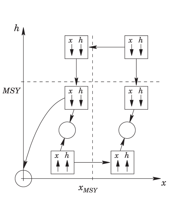
Figure 3: State-transition graph (STG) for the solution set of the naïve model. The arrows in the vertices (boxes) indicate the qualitative direction of the relevant variables: $h$: harvest and $x$: stock. The position in the diagram refers to the qualitative magnitude, and the arrows between the boxes describe possible changes of qualitative states in time. Circles represent equilibrium states. All states with a qualitative magnitude of $h>MSY$ are characterized by a decreasing stock and harvest. Below the $MSY$ level $x$ and $h$ both decrease or increase. One of the equilibria represents extinction ($x=h=0$), one a steady state below $x_{MSY}$, another an equilibrium above this landmark.

Comparing the QDE method with Monte Carlo simulations or Markov chains, one has to emphasize that it is a deterministic approach. In contrast to probabilistic methods, qualitative modelling determines possible transitions for the systems development in the logical sense. This is quite different to techniques propagating changes on the basis of likelihoods, e.g. by transition matrices (for an example of such approaches cf. Erev and Roth, 1998). It is in general not possible to derive probabilities in the case of multiple successors of a single state, since these also depend on qualitative states visited before (the Markov property is violated). Furthermore, due to various uncertainties, it is often impossible to measure sufficient frequency records. A QDE is a compact representation of a large family of ODEs, and the simulation result includes all their solutions. The result is rather general in nature, since no parameters need to be specified. Therefore, the result of qualitative simulation is not exactly the same as of common phase-plane analysis. There, multiple cases due to the number of intersections of the main isoclines (where the derivatives of some state variables vanish) have to be specified (as in, e.g. Cropper et al., 1979) – depending on the concrete parameterization, which is not known to the modeller in our case. For the same reasons, different cases regarding stability of equilibria, bifurcations and other phenomena studied in nonlinear analysis are contained in one qualitative model. In the STG one circle may represent multiple equilibria of different types. If the modeller wants to exclude or distinguish some cases, additional equilibria must be made explicit by introducing new landmarks and linking them with appropriate constraints.

3 A Fishery Model with Capital Accumulation

In this section we introduce a bio-economic model describing a situation where $N$ identical and profit-maximizing firms compete for an unregulated resource, i.e. a marine fish stock with the size $x$. Because the harvesting technology and the associated cost and profit functions have been formulated in several ways in the previous literature (Clark et al., 1979; McKelvey, 1985; Boyce, 1995; Amundsen et al., 1995), we start by deriving a generic formulation based on standard production economics. Assume that any harvesting requires variable inputs (labour, fuel, material), jointly referred to as effort $e$, and fixed inputs $k$ (capital, e.g. ships and gear). The productivity of these inputs depends on the biological stock $x$. Thus, a production function $f(e,x,k)$ can be defined, that determines the resulting harvest $h\geq 0$. For its partial derivatives the properties $f_{e},f_{x},f_{k}>0$, $f_{ee},f_{kk},f_{xx}<0$, $f_{ex},f_{ek},f_{xk}>0$ are imposed. The first two sets of inequalities describe the standard properties of positive, decreasing marginal productivity. The third set of inequalities means that the marginal product of the variable input decreases with decreasing fish stock, but is raised by capital accumulation. The derivative of harvest with respect to the fish stock also increases in capital, because certain attributes of capital enhance the accessibility of the fish stock (improved fishing gear and technology, increased horsepower of boats, etc.).

Since $x$ and $k$ are given when a firm undertakes efforts $e$ to obtain a chosen $h$, the resulting variable costs $v$ depend on $h,x$ and $k$. The function $v(h,x,k)$ can be determined by solving $h=f(e,x,k)$ for $e$ and multiplying it with a renumeration rate $w$ which is assumed to be fixed. Due to the assumptions made for $f$, the implicit function theorem implies that

$$v_{h}>0,v_{x},v_{k} <0,$$

$$v_{hh},v_{kk},v_{xx},v_{kx} >0,$$ (12)

$$v_{hx},v_{hk} <0.$$

Additionally, we assume that the Hessian of $v$ is positive definite, which is no contradiction to the above inequalities. This guarantees usual convexity properties as needed later on. It should be noted that the marginal harvesting costs $v_{h}$ decrease in both the fish stock and the capital stock. This assumption differs from previous approaches where capital only sets an upper limit for the harvest, such that an increase in capital equipment improves the productivity of the variable inputs, and capital accumulation may offset the negative effect of a declining fish stock on harvesting costs.

We now turn to the dynamics of the economic and biological stock. The regeneration of the resource is given by a concave recruitment function $R(x)$, for which the assumptions made in section 2 are valid. We define

$$\dot{x}=R(x)-(h+h^{\prime})$$ (13)

as the equation of motion, where $h$ denotes the harvest of a firm under consideration and $h^{\prime}$ that of all the others. Each firm’s capital stock is described by

$$\dot{k}=I-\delta k,$$ (14)

where $I\geq 0$ represents (irreversible) investment and $\delta$ the depreciation rate which is assumed to be constant. Investment costs are expressed by a strictly convex increasing function $c(I)$. The convexity reflects inelastic supply of highly specialized equipment and rising adjustment costs for higher investment. The demand for fish is described by the downward sloping inverse demand function $p(h+h^{\prime})$.

In the following the decision of each firm on $h$ and $I$ has to be determined. If each fishing company acts in an economically rational way, it chooses an investment and harvest plan that maximizes the discounted profit given by

$$\Pi:=\int_{J}e^{-rt}\bigg{(}p(h+h^{\prime})h-v(h,x,k)-c(I)\bigg{)}dt$$ (15)

subject to Eq. (13) and Eq. (14). Here, $r$ denotes a constant discount rate and $J=[0,T]$ a planning interval.

The optimization problem can be solved by a sufficiency theorem of Mangasarian (1966). By introducing $\lambda$ and $\mu$ as costate variables for $x$ and $k$, the current-value Lagrangian is given by

$$L=p(h+h^{\prime})h-v(h,x,k)-c(I)+\lambda\big{(}R(x)-(h+h^{\prime})\big{)}+\mu\big{(}I-\delta k\big{)}+\sigma_{1}h+\sigma_{2}I+\sigma_{3}x+\sigma_{4}k.$$ (16)

The four slack variables appear due to the constraints $I,h,x,k\geq 0$. Since $L$ is concave in $(x,k)$, an interior solution to the first-order conditions $L_{h}=L_{I}=0$ and the costate conditions $L_{x}=r\lambda-\dot{\lambda}$ and $L_{k}=r\mu-\dot{\mu}$ (where $\sigma_{1}=\sigma_{2}=\sigma_{3}=\sigma_{4}=0$) with $\lambda,\mu\geq 0$ and $\lambda(T)=\mu(T)=0$ is an optimal path. We assume that marginal investment costs become small for a low investment level, i.e. $c_{I}(0)=0$, avoiding that there is a negative solution of $L_{I}=-c_{I}(I)+\mu=0$ since $c_{II}>0$. It is not as easy to guarantee a non-negative solution of $L_{h}=0$, which depends on the relation between prices and variable costs. However, we do not investigate the optimal path in detail since it may be unrealistic because firms are most likely to ignore the effect of their harvesting decision on future stocks (Harris, 1998; Banks, 1999; Hatcher, 2000). In other words, they disregard Eq. (13) in their optimization procedure, partly because of a lack of knowledge on the recruitment function, and partly because they consider their own influence on the fish stock to be negligible. Moreover, they tend to assume that other firms behave in the same way. Thus, we suppose that the shadow price for the biological stock is neglected by the individual firms. We further assume that the number of firms is constant and investment takes place in the form of increasing fishing power or number of vessels per firm. From this perspective it is consistent to set $\lambda\equiv 0$ in the fourth summand of the current-value Hamiltonian Eq. (16). As a consequence, the costate condition for $\lambda$ is ignored and corner solutions of $H_{h}=0$ become irrelevant. The harvest decision is myopic in contrast to the investment decision. Utilizing the (constant) inverse price elasticity of demand $\epsilon<1$, one obtains the following equations:

$$L_{h} =\bigg{(}1-\epsilon\frac{h}{h+h^{\prime}}\bigg{)}p(h+h^{\prime})-v_{h}=0,$$ (17)

$$L_{I} =-c_{I}(I)+\mu=0,$$ (18)

$$L_{k} =-v_{k}-\mu\delta=r\mu-\dot{\mu}.$$ (19)

According to Eq. (18) the costate variable on capital equals the marginal cost of investment. If the latter were constant, as assumed in several previous models, Eq. (19) would therefore boil down to the usual condition that the user cost of capital, $(r+\delta)c_{I}$, should just be balanced by the induced reduction in variable costs, $-v_{k}$. In our model with increasing marginal investment costs we get a more complicated equation. By substituting $\mu$ from Eq. (18) and its time derivative in Eq. (19) one gets $(r+\delta)c_{I}=-v_{k}+\dot{c_{I}}$, where $\dot{c_{I}}=c_{II}\dot{I}$. The investment programme is characterized by the condition that the user cost of capital should be balanced not only by reduced variable costs, but also by the change in the purchase cost of capital induced by a change in the level of investment.

Because we have assumed that all firms are characterized by the same technology and behave in the same way, one obtains $h+h^{\prime}=Nh$. Consequently, the total amount of capital and investment is given by $N\cdot k$ and $N\cdot I$, respectively. Our model can therefore be written in the following way:

$$\dot{x} =R(x)-Nh,$$ (20)

$$v_{h} =\bigg{(}1-\frac{\epsilon}{N}\bigg{)}p(Nh),$$ (21)

$$\dot{I} =\frac{1}{c_{II}(I)}\big{(}(r+\delta)c_{I}(I)+v_{k}\big{)},$$ (22)

$$\dot{k} =I-\delta k.$$ (23)

Equation (22) has already been interpreted above and Eq. (21) represents the usual equality between marginal variable costs and marginal revenue. It should be recalled that the marginal variable costs $v_{h}$ decrease in both the fish stock and the capital stock. Therefore, an increase in marginal costs due to a decreasing fish stock may trigger additional investment in an effort to keep marginal costs from rising excessively. This is crucial for explaining why the capital stock may increase along with a decrease in the fish stock, a phenomenon which is at the heart of what is frequently referred to as over-capitalization. We will show in the next section that this happens for every parameterization of the model.

To analyse whether over-capacities occur or not, and whether the fish stock recovers once it is in a critical state, we are interested in the dynamics of the ODE model Eq. (20)–(23) far from equilibrium. Due to the difficulties with phase-plane analysis and numerical simulation as discussed before, we study the QDE corresponding to the model in the next sections.

4 The Qualitative Model and its Solution

4.1 Abstraction of the Analytical Model

The abstraction procedure commences as outlined in section 2. At first, landmarks for all variables are chosen and constraints about the functions are defined. For the resource stock $x$, recruitment $R$ and harvest $h$ the same landmarks as in section 2 are introduced. The constraints relating $x$ to $R$ and $\dot{x}$ to $R$ and $h$ are the same as given in (3)–(10) and (26). For capital and investment the landmarks $k:0<k_{max}$ and $I:0<I_{max}$ are defined. Further descriptions of the following constraints are provided in the annex.

Eq. (21) for the marginal variable costs $v_{h}$ can be solved for $h$ to yield a harvest supply function $h(x,k)$. This function is increasing in both arguments, which can be shown from the assumptions made for the production function $f(e,x,h)$ and the inverse demand function $p$, which implies

$$\quad\text{if}\quad\dot{x}>0 \dot{k}>0 \dot{h}>0,$$ and then (24)

$$\quad\text{if}\quad\dot{x}<0 \dot{k}<0 \dot{h}<0.$$ and then

The constraints following from Eq. (12) for $v_{k}$ are given by (27), those from Eqs. (22) and (23) by (28)–(29) (cf. annex). For technical reasons $v_{k}$ is replaced by $-v_{k}:-v_{k_{max}}<0$. This implies that $-v_{k}$ can be expressed by a function which is strictly monotonically increasing in $h$ and strictly monotonically decreasing in $x$ and in $k$ (cf. Eq. (12)). Further on, we assume that $c_{II},r$ and $\delta$ are constant. Since $c_{I}(0)=0$, it can be shown that $I$ has always the same sign and qualitative direction as the expression $\frac{r+\delta}{c_{II}}c_{I}(I)$. Therefore, this term of Eq. (22) can be simplified to $I$ qualitatively. For the same reason $\delta\cdot k$ can be replaced by $k$ (in Eq. 22), and $N\cdot h$ by $h$ (in Eq. 20). Thus, the abstraction of the model and the associated constraints as given by Eqs. (20)–(23) can be expressed in the following relational form, where the right hand side represents the typical notation developed by Kuipers (1994, cf. annex for further details):

$$\dot{x}+h =R \equiv\quad$$ ((add dx h R)(0 0 0)(0 MSY Rmsy))

$$R(x) =R \equiv\quad$$ ((U- x R)(0 0)(xmsy Rmsy)(Q 0))

$$h(x,k) =h \equiv\quad$$ (((M++) x k h)) (25)

$$\dot{k}+k =I \equiv\quad$$ ((add dk k I))

$$\dot{I}+(-v_{k}) =I \equiv\quad$$ ((add dI mvk I))

$$f(h,x,k) =-v_{k} \quad\equiv\quad$$ (((M-++) h x k mvk))

The constraint add is the qualitative abstraction of quantitative addition. The U- constraint represents a downward bent U-shaped function of logistic type (cf. annex). The landmarks in the brackets are corresponding pairs/triples of argument and result values specifying correspondences between variables, e.g. in the first equation of (25): if $\dot{x}=0$ and $h=MSY$, then $R=R_{MSY}$.

4.2 Results

The qualitative simulation of the bio-economic model (see footnote 2) provides 467 qualitative states. According to the methodology described in section 2 the potential systems developments are structured and reorganized as a GSTG (Fig. 4) with stock size, harvest and capital as relevant variables.

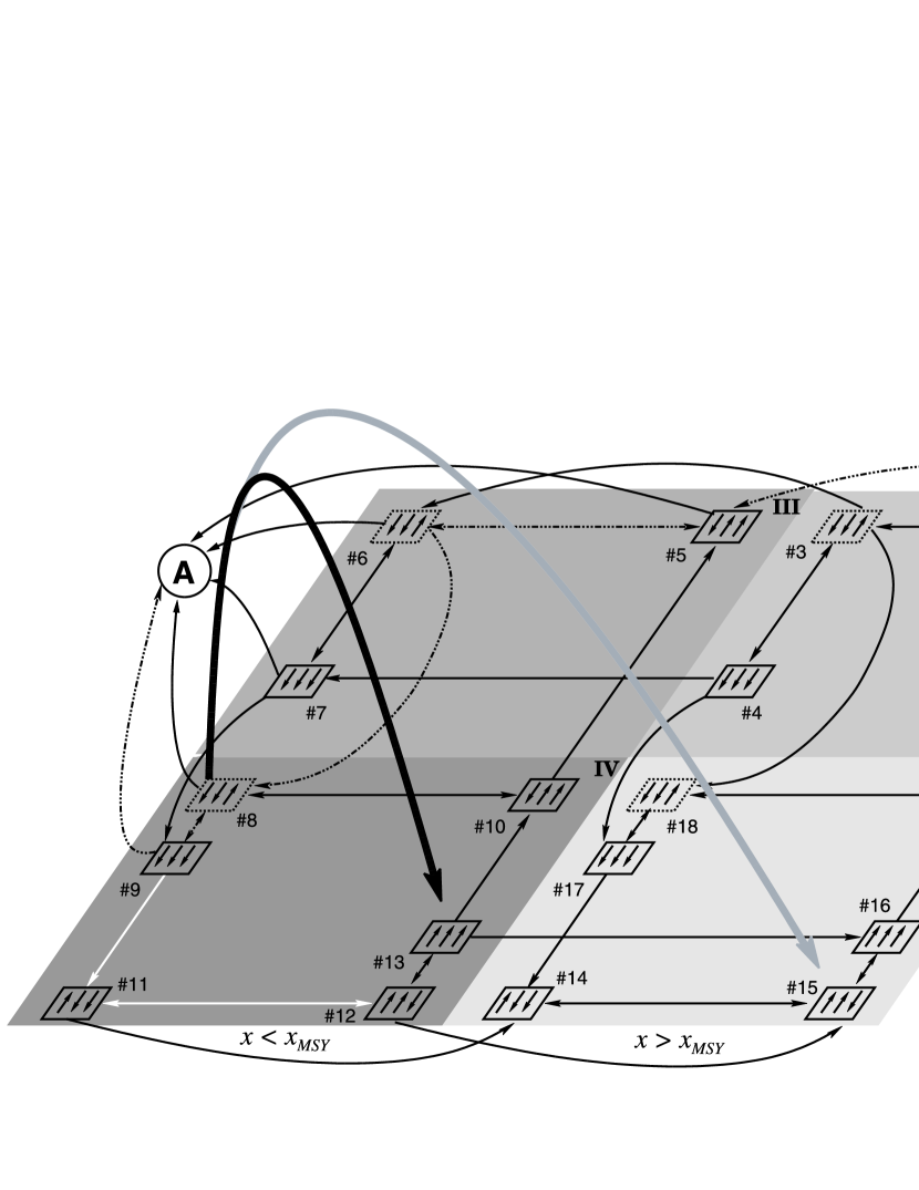
Figure 4: Solutions of the qualitative model represented as GSTG. The arrows in the vertices label the direction of the first derivative (from left to right $\dot{x},\dot{h},\dot{k}$), the dashed boxes indicate situations where over-capitalization occurs. Arrows between vertices indicate possible transitions. The dashed and the white arrows indicate typical development paths (cf. text). The two bold arrows indicate management interventions as discussed in section 5.1.

The GSTG contains 19 vertices, where one $\bigcirc$A , represents a catastrophic equilibrium (where $x=0$). For each behaviour represented in the GSTG, corresponding phase plots for the relevant variables are available. Now, the question about the real-world validity of these trajectories and the added value for the discussion of the problems in fisheries arises. Our argumentation follows three directions:

• In order to validate the results obtained it can be checked whether case studies can be reconstructed by observed time behaviours. As an example we discuss the development of the blue whale fishery in the time period 1946-1980 (Fig. 5).

• The qualitative approach determines all ‘dynamic patterns’ which are conceivable under the model settings. The GSTG enables us to determine general properties common to all time developments.

• The GSTG has the capabilities to discuss potential management interventions, e.g. for scenario analysis or for detection of serious developments. In this sense the approach supplies knowledge for an ex-ante assessment.

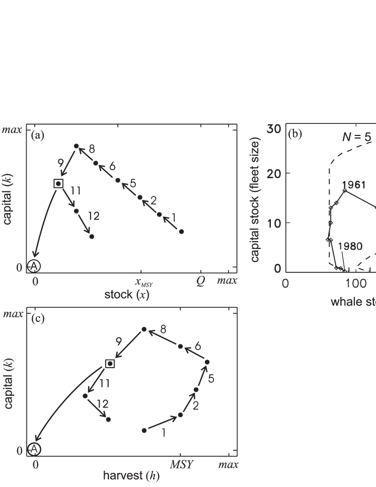
Figure 5: Qualitative phase plots for two critical developments observable in fisheries (a,c). The boxed dot refers to a critical branching, where the resource stock either vanishes or recovers. The numbers correspond to the qualitative states in Fig. 4. (b) displays the situation in the blue whale hunting industry from 1946–1980 (BWU $\equiv$ blue whale units; the dashed lines refer to model outputs generated by the  McKelvey (1986) model, and $N$ to the number of firms in this model).

The example of blue whale fishery (Fig. 5b) shows that the qualitative bio-economic model fits real situations quite well. Figures 5a and 5c display the associated phase plots of the qualitative model, indicating a development path corresponding to transitions from vertex #1 to #12 (Fig. 4, dashed-dotted and white arrows). Both the observed quantitative and the qualitative case are characterized by an initial expansion phase where the whale stock declines while the capital stock increases. This is followed by a period in which the capital stock declines rapidly, while the whale stock is still declining. Finally, the capital decreases further, whereas the stock tardily recovers. This is completely different to several models (e.g. Clark et al. 1979, McKelvey 1986, cf. Fig. 5b) which, due to linearity assumptions, show an initial and a final jump of the capital stock.

Since the GSTG contains many paths, we may wonder if every fishery showing an intial expansion phase can be reconstructed by the model. However, in the following we identify further structural properties of the graph – the model can only explain real-world fisheries which reflect these patterns. During the expansion phase the stock decreases while capital is still increasing. In the course of further evolution the effect of declining stocks on harvesting costs becomes so important that it cannot compensated any longer by investment. Then the capital stock begins to decrease, i.e. net investment $I-\delta k$ becomes negative. At this stage it is possible (Fig. 5a) that the fish stock approaches zero (a discussion of such branching points is provided in section 5.2.). However, it is also possible that the decline of the fish stock is reversed. In contrast to models like those of Clark et al. (1979) and McKelvey (1986), in this case fisheries do not need to attain an equilibrium with $x>0$, but can exhibit a further boom-and-bust cycle through all quadrants. It is not even safeguarded that the system converges to an equilibrium after repeated cycles.

We can also show that every fishery described by the model necessarily undergoes a phase of over-capitalization. This is related to the fact that via the simulation irreversible transitions are identified, i.e. transitions between qualitative states which are possible only in one direction (cf. GSTG, e.g., from quadrant II to quadrant III). The proof of this proposition is as follows: decreasing catches and increasing capital stock occur simultaneously, whenever the system approaches the critical vertices #3, #6, #8 or #18. If the system starts, for example, at vertex #1 (relatively undisturbed stock) and does not directly shift to vertex #18, the only way to avoid vertex #3 is to change from vertex #2 to #5. However, at #5 the only way for a further development (without collapse of the stock) is via vertex #6. Thus, we always approach at least one of the critical vertices and in this sense over-capitalization is an unavoidable system property. This property is rooted in the fact that $v_{hx}<0$ and $v_{hk}<0$, i.e. that the harvest supply function increases in $x$ and $k$ (via Eq. (21)). As long as we observe increasing harvest although the fish stock is reduced, net investment must be positive to compensate losses from increasing marginal costs. Therefore, $k$ cannot start to decrease before $h$.

5 Discussion and Policy Implications

Discussing the results and implications for policy actions, a variety of conclusions can be drawn. The model is further validated by showing that mistakes arising from temporary management measures can be reconstructed by the model.

5.1 Why Management Fails

Public decision makers may respond rather late to an emerging crisis and, in addition, with drastic, but temporary interventions. Such situations can be analysed with the model as follows: although the system does not follow the dynamics of an unregulated fishery during a period managed in this way, we can compare the qualitative state of the system before and after this time frame. Two such interventions are represented by the bold arrows in Fig. 4 starting at the dashed vertex #8 and addressing the well-known problems in the cod fisheries of the North Atlantic ocean (Grand Bank and Barents Sea). The situation in the Grand Bank region and in the Barents Sea exhibited similarities, but the results of political interventions in these two cases were different. Whereas in the Canadian case the worst consequences ensued, the Norwegian authorities were able to prevent a severe disaster. The question arises, how and why?

The cod fiasco in the Canadian waters at the beginning of the 1970s is an example of an maladjusted strategy leading to a severe economic and environmental catastrophe.

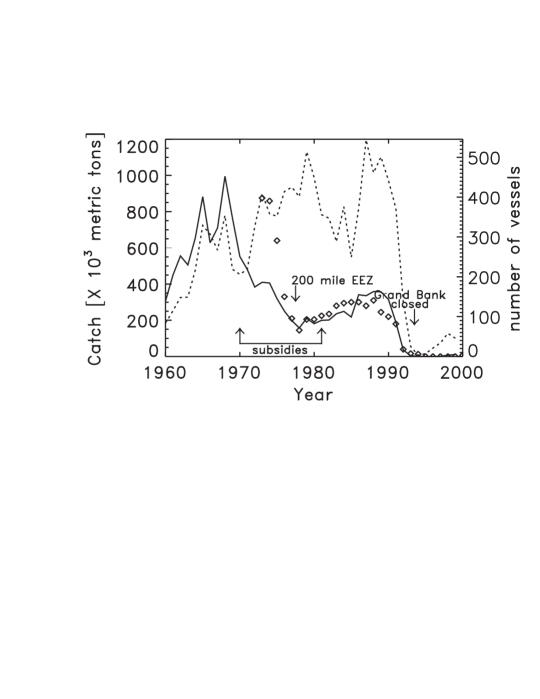
Figure 6: Catch of Atlantic cod in the area of the Northwest Atlantic Fishery Organization (Newfoundland, Grand Banks, area 2J3KL). The dashed line indicates the increase in number of vessels (all countries targeting cod (gadus morhua)) operating in this area and the diamonds the total allowable catch (data from NAFO, 2002; DFO, 2002).

Anticipating an ecological disaster, the exclusive economic zone (EEZ) was introduced in 1977 and foreign trawlers were banned from the Grand Banks. The government implemented catch quotas which, however, were not always binding. In parallel, the government responded with massive subsidies to the fishery. The earliest situation when such a situation occurs in the GSTG is at vertex #6 where the harvest is above the sustainable level and the stock already below. The only way to avoid more serious developments is to alter to vertex #7 (and from there to #9, #11, etc.), but this needs a reduction of the capital. Indeed the Canadians did just the opposite, i.e. the awareness of increasing gains due to the ban on European trawlers led to investment in improved gear and to more efficient fish killing (Harris, 1998). The situation at the end of the 1970s is represented by vertex #8 (Fig. 4), where both stocks and catches are below a critical level and still decreasing while the capital continues to increase. The reaction of the government in this situation was counterproductive (cf. bold black arrow in Fig. 4). It may be that the stocks slightly recovered (possibly indicated by an increased catch, cf. Fig. 6), but they have not reached a sustainable level (i.e. $x_{MSY}$). Thus, when the total allowable catches (TAC) were relieved, the system was not in a safe state, but approached a state represented in the model results by vertex #13. A second period of high catch levels occurred, which led to the critical state #8 again (along the path #13–#10–#8 or via #13–#10–#5–#6–#8), finally approaching $\bigcirc$A  via # 9. This was the end of the story, because the cod stock has not recovered up to the present day.

To prevent these short-termed cycles, it would be better to shift the system to vertex #15. This was the case in Norway when the country faced a similar disaster in the Barents Sea. Here, individual transferable quotas helped to reduce the race for fish. Although there were a lot of bankruptcies in fisheries and many demonstrations, the politicians knew that there could be no giving in to protests for short-term political gain. They set up subsidies – in contrast to the Canadians – to remove ships from fisheries and to diversify the coastal economy (Harris, 1998). Finally, they banned fishing from spawning grounds. This is equivalent to a path sequence via #8–#9–#11–#14–#15. Thus, Norway now has a better basic position for a sustainable resource management. However, a slackening of catch permits, as currently discussed, may lead to the outcome that the unregulated dynamics starts again at vertex #15. We conclude from these two cases that short-term measures or non-binding catch quotas only suspend the intrinsic problem.

5.2 Scenario Assessment and Critical Branchings

The GSTG provides various clues on how management interventions can be implemented. Although some of them may not differ so much from earlier conclusions (cf. those derived from the static model of Gordon, 1954), they are here based on a comprehensive system analytical background and a full dynamical perspective. For example, irreversible transitions indicate critical stages in the development of the fishery. The fishery is in a ‘high-risk situation’ when stock and harvest are decreasing, but capital is still increasing and if at least one irreversible transition occurred (from #3 to #6, or form #4 to #7). Critical branchings are states characterized by multiple successors, where at least one of them is an irreversible transition. Here, either a worsening or mitigation is possible (e.g. #1, #2, #4, #9, or #13). Fishery management can use the information represented by the GSTG and take account of the fisheries’ problems in two ways:

1. How can it be avoided that the fishery returns again to critical branching after the resource has recovered?

2. Under which conditions can critical branchings be prevented at an early stage, i.e. that the system does not leave quadrants I and II?

We can consider control measures for harvest, capital, or stock, but also - in a qualitative sense - the time when they have to be applied at the latest. It would also be helpful to assign likelihoods to different transitions at these branchings. Although results of the latter kind are problematic in this context (cf. Sect. 2, last paragraph), the qualitative model provides a starting point for investigations in this direction. We illustrate these issues by referring again to the example of the blue whale fishery (dashed-dotted arrows, Fig. 4). Assume that we start with a relatively undisturbed stock and an industry at a low level (#1, quadrant I, $x>x_{MSY},h<MSY,\dot{x}<0,\dot{h}>0,\dot{k}>0$). The first irreversible transition occurs from vertex #1 to #2 (quadrant II). Already here the catch exceeds the sustainable level ($h>MSY$), while the capital stock is still increasing. To avoid such a situation, strong harvest limitations must be introduced, i.e. the harvest rate must decrease before $MSY$ is reached and the stock approaches $x_{MSY}$, while over-capitalization might continue. For such a transition to node #18 the following scenario is conceivable: the harvest costs already strongly increase due to a reduced population although it is still above $x_{MSY}$ and/or the substitution of resource by capital stock has only minor effects. In reality this is observable for less developed fisheries. For highly developed fisheries the system evolves to vertex #2 (quadrant II, $x>x_{MSY},~{}h>MSY,~{}\dot{x}<0,~{}\dot{h}>0,~{}\dot{k}>0$, cf. Fig. 5) representing fisheries having the potential to increase harvest and capital (as, for instance, the blue whale fisheries between 1946-1960). A safe development under these conditions can only be guaranteed if a transition to vertex #5 or #6 is avoided. At vertex #2 this is possible via #3, where we are still in quadrant II, but the situation is economically worse than at vertex #2, because in addition to declining fish stocks, harvest is also decreasing. Sustainable limits can only be reached by massive harvest limitations (evolution via #4–#17). If these actions are not implemented, the transition to #5 or #6 is inescapable and fisheries necessarily enter to a situation in which the industry and the fish stock are likely to be ruined $\bigcirc$A . The further development depends on how early net investment decreases, i.e. in the phase when quadrant III is reached, effort controls are more important than catch controls. In contrast in quadrant IV, successful recovery is determined by the regeneration rate of the fish stock and the speed of harvest reduction. Since policy actions often have the tendency to come into play too late, over-capitalization and therefore over-exploitation is a permanent risk. Qualitative simulation shows that at these vertices the collapse of the fishery can be prevented if, due to a rapid capital reduction, the stock already recovers (indicated by the white arrows, Fig. 4). In general the simulation results indicate that fisheries under the settings of the model are in a state of perpetual risk, because the high risk states (#5–#9) are likely to occur repeatedly in every boom-and-bust cycle.

We conclude that – if it is impossible to formulate a precise numerical model – qualitative simulation has complementary advantages compared to other methods. First, we can shift the perspective from equilibria to non-equilibrium dynamics and can unveil general dynamic patterns, i.e. intrinsic properties of unregulated fisheries which hold for every functional and parametric specification of the model and which cannot be identified by comparative dynamics in a neighbourhood of the equilibrium. Examples are unavoidable overcapacities and the possibility of cyclical behaviour. Second, several stages of system development can be identified to enhance our knowledge of how and when management strategies should be introduced. This allows alternative scenarios to be discussed. Third, critical branchings were identified. These can be associated with regions in the phase space where the qualitative direction of state variables are in a configuration which admits irreversible problematic and positive changes. In our model, factors for the propensity of the system to recover include (cf. Eqs. (20)–(23)): (i) regeneration rate of the fish stock, (ii) depreciation of the capital stock, (iii) marginal investment costs and (iv) marginal variable costs with respect to capital and harvest. Here, qualitative reasoning comes to its limits, since no numerical estimates for critical parameters can be made. Yet we think that the method helps to identify decisive regions of the phase space as a starting point for the development of new hypotheses focusing specifically on them. Semi-quantitative techniques combining qualitative and quantitative methods show promise here (cf. Berleant and Kuipers, 1998). Thus, qualitative reasoning is appropriate whenever we are dealing with imprecise knowledge. Given the complexity of the systems in question it must be accepted that one may have to be content with “soft prognoses” only.

6 Conclusion

This paper addresses the global problem of industrial unregulated fisheries and the role of capital accumulation. Such systems are often intrinsically complex and the understanding of them is limited by low levels of knowledge with respect to both biological and economic properties. To keep models tractable, previous analytical approaches have relied on a variety of simplifying assumptions with respect to investment costs, harvesting costs or industry structure. Additionally, they often concentrated on equilibrium analysis or on comparative dynamics near equilibrium. We demonstrated qualitative modelling as a new method to approach uncertainty and tractability problems by applying it to a model which improves former results by relaxing assumptions. The qualitative model describes the dynamical behaviour of a fishery without reference to quantitative values. We have shown that this technique can improve our reasoning about global properties of the dynamics of the system.

The model features (i) increasing marginal investment costs and (ii) marginal harvesting costs that are decreasing in both the fish and the capital stock. Due to the former, the build-up of fishing capacities can be modelled more realistically. Due to the latter, fish stock and capital stock are (incomplete) substitutes in the production of catch. This proved to be the key factor in explaining why capital will keep rising while both the fish stock and the catch decline. The qualitative simulation reveals that all fisheries described by the general model necessarily undergo a phase of over-capitalization. It also shows other inherent and – in the sense of political interventions – serious system properties, e.g. critical branchings and potentially recurring boom-and-bust cycles.

Future work will run along several lines. Different policy measures can be assessed by incorporating them into the qualitative model and comparing the resulting graphs. Also a multi-species module, together with more detailed models of decision making in fisheries could enhance the results. Some other efforts are related to an integration of hard and soft knowledge in one model approach. In particular model approaches comprising a module for cooperative negotiations and allows to test which management strategies are applicable in a fishery under additional settings, e.g. normative sustainability targets, are examined (see, e.g. Kropp et al., 2004; Eisenack et al., 2005). Summing up, we feel that the results and the technique open a promising road towards new insights in the dynamics and management of fishery systems.

Acknowledgements: This work was supported by the German Federal Ministry for Education and Research (BMBF) under grant number 03F0205B (DIWA). We wish to thank the anonymous reviewers for their helpful comments.

Appendix A Annex

The annex completes the qualitative constraints derived from the bio-economic model (cf. Eqs. (20)–(23)) and the assumptions made in section 3. These constraints are translated to the specific model code necessary to run the qualitative simulation software.

The relationship between stock $x$ and harvest $h$ is defined by the relations in Eq. (3) and expressed by constraint (C.1a) in the subsequent table. The recruitment is given by a U-shaped function $R(x)$, defined in Eqs. (4)–(9) and expressed by constraint (C.1b). To describe the change of fish stock $\dot{x}=R-h$, the complete model needs more than Eq. (10). The derivative $\dot{x}$ is increasing with $R$ and decreasing with $h$. In addition, if $h$ becomes zero, $\dot{x}$ changes in the same direction as $R$ and if $R$ vanishes, $\dot{x}$ changes in the opposite direction to $h$. Since $R_{MSY}=MSY$, $\dot{x}=0$ if $R=R_{MSY}$ and $h=MSY$:

if $$R=0 \text{and}\quad h=0 \dot{x}=0,$$ then

if $$R=R_{MSY} \text{and}\quad h=MSY \dot{x}=0,$$ then

if $$R<R_{MSY} \text{and}\quad h>MSY \dot{x}>0,$$ then (26)

if $$\dot{R}>0 \text{and}\quad\dot{h}<0 \ddot{x}>0,$$ then

if $$\dot{R}<0 \text{and}\quad\dot{h}>0 \ddot{x}<0.$$ then

These expressions are equivalent to those which are encoded in the qualitative constraint (C.1c). The constraints for the harvest supply function $h(x,k)$ are already defined in Eq. (24) and expressed by constraint (C.2a). In addition, Eq. (12) states that the negative marginal costs $-v_{k}$ increase in $h$ and decrease in $x$ and $k$. Thus,

$$\begin{split}\text{if}\quad\dot{h}>0\quad\text{and}\quad&\dot{x}<0\quad\text{and}\quad\dot{k}<0\quad\text{then}\quad-\dot{v_{k}}>0,\\ \text{if}\quad\dot{h}<0\quad\text{and}\quad&\dot{x}>0\quad\text{and}\quad\dot{k}>0\quad\text{then}\quad-\dot{v_{k}}<0,\\ \end{split}$$ (27)

which is expressed by the constraint (C.2b), where $v_{k}$ is replaced by $mv_{k}:=-v_{k}$ for technical reasons. Taking into account Eq. (23) it is obvious that the change of capital stock is increasing with $I$ and decreasing with $k$. If $k$ vanishes, $\dot{k}$ changes in the same direction as $I$, if $I$ vanishes, $\dot{k}$ changes in the opposite direction to $k$, yielding

if $$I=0 k=0 \dot{k}=0,$$ and then

if $$\dot{I}>0 \dot{k}<0 \ddot{k}>0,$$ and then

if $$\dot{I}<0 \dot{k}>0 \ddot{k}<0,$$ and then (28)

if $$\dot{I}=0 sgn(\ddot{k})=-sgn(\dot{k}),$$ then

if $$\dot{k}=0 sgn(\ddot{k})=sgn(\dot{I}).$$ then

The relationship between $\dot{k}$ and $I$ is represented by (C.3). Finally, referring to Eq. (22), the change of investment has the form $\dot{I}=f(I)+g(v_{k})$ with strictly monotonic increasing functions $f$ and $g$ which vanish at zero. Thus,

$$\text{if}\quad I=0 v_{k}=0 \dot{I}=0,$$ and then

$$\text{if}\quad\dot{I}>0 \dot{v_{k}}>0 \ddot{I}>0,$$ and then

$$\text{if}\quad\dot{I}<0 \dot{v_{k}}<0 \ddot{I}<0,$$ and then (29)

$$\text{if}\quad\dot{I}=0 sgn(\ddot{I})=sgn(\dot{v_{k}}),$$ then

$$\text{if}\quad\dot{v_{k}}=0 sgn(\ddot{I})=sgn(\dot{I}),$$ then

which is encoded in the constraint (C.4). Again we change $v_{k}$ to $-v_{k}$. The constraints, expressed by a set of comprehensible and recurring keywords, are summarized in the following table:

Index	Example	Interpretation
(C.1a)	((M+ x h) (0 0))	$\exists f:h=f(x),f(0)=0,f_{x}(x)>0$
(C.1b)	((U- x R) (xmsy Rmsy) (0 0) (Q 0))	$\exists f:R=f(x),f(x_{MSY})=R_{MSY},f(0)=0,$
		$f(Q)=0;\forall x<x_{MSY}:f_{x}(x)>0;$
		$\forall x>x_{MSY}:f_{x}(x)<0.$
(C.1c)	((add dx h R) (0 0 0) (0 MSY Rmsy))	$\dot{x}+h=R\equiv\dot{x}=R-h,0+MSY=R_{MSY}$
(C.2a)	(((M + +) k x h))	$\exists f:h=f(x,k),f_{k}>0,f_{x}>0$
(C.2b)	(((M - + +) h x k mvk))	$\exists f:-v_{k}=f(h,x,k),f_{h}<0,f_{x}>0,f_{k}>0$
(C.3)	((add dk k I) (0 0 0))	$\dot{k}+k=I\Leftrightarrow\dot{k}=I-k$
(C.4)	((add dI mvk I) (0 0 0))	$\dot{I}+{(-v_{k})}=I$
Additional constraints for derivatives and exclusion of marginal cases are:
(C.5)	((d/dt x dx))	$\dot{x}=\frac{d}{dt}x$
(C.6)	((cornot x dx) (xmsy 0))	$\forall t:x(t)\neq x_{MSY}\vee\dot{x}(t)\neq 0$,
		i.e. it is forbidden that $x=x_{MSY}$ and
		$\dot{x}=0$ at the same time

References

- Amundsen et al. (1995) Amundsen, E. S., Bjørndal, T., Conrad, J. M., 1995. Open access harvesting of the Northeast Atlantic minke whale. Environmental and Resource Economics 6, 167–185.
- Banks (1999) Banks, R., 1999. Subsidising EU fleets: capacity reduction or capital subsidisation. In: Hatcher, A., Robinson, K. (Eds.), Overcapacity, Overcapitalisation and Subsidies in European Fisheries. cemare, Portsmouth, pp. 200–210.
- Benaroch and Dhar (1995) Benaroch, M., Dhar, V., 1995. Controlling the complexity of investment decisions using qualitative reasoning techniques. Decision Support Systems 15 (2), 115–131.
- Berck and Perloff (1984) Berck, P., Perloff, J. M., 1984. An open-access fishery with rational expectations. Econometrica (2), 489–506.
- Berleant and Kuipers (1998) Berleant, D., Kuipers, B. J., 1998. Qualitative and quantitative simulation: Bridging the gap. Artificial Intelligence 95 (2), 215–255.
- Boyce (1995) Boyce, J. R., 1995. Optimal capital accumulation in a fishery: A nonlinear irreversible investment model 28, 324–339.
- Bredeweg and Salles (2003) Bredeweg, B., Salles, P., 2003. Qualitative reasoning about population and community ecology. Artificial Intelligence 24 (4), 77–90.
- Caputo (1989) Caputo, M. R., 1989. The qualitative content of renewable resource models. Natural Resource Modeling 3 (2), 241–259.
- Caputo (2003) Caputo, M. R., 2003. The comparative dynamics of closed-loop controls for discounted infinite horizon optimal control problems. Journal of Economic Dynamics and Control 27 (8), 1335–1365.
- Charles (2001) Charles, A., 2001. Sustainable Fishery Systems. Blackwell.
- Clark (1999) Clark, C. W., 1999. Renewable resources: fisheries. In: van den Bergh, J. C. J. M. (Ed.), Handbook of Environmental and Resource Economics. Edward Elgar Publishers.
- Clark et al. (1979) Clark, C. W., Clarke, F. H., Munro, G. R., 1979. The optimal exploitation of renewable resource stocks: poblems of irreversible investment. Econometrica 47, 25–47.
- Cropper et al. (1979) Cropper, M. L., Lee, D. R., Pannu, S. S., 1979. The optimal extinction of a renewable natural resource. Journal of Environmental Economics and Management 6, 341–349.
- de Kleer and Brown (1984) de Kleer, J., Brown, J. S., 1984. A qualitative physics based on confluences. Artifical Intelligence 24, 7–83.
- Dechter (2003) Dechter, R. (Ed.), 2003. Constraint Processing. Morgan Kaufmann, San Mateo.
- DFO (2002) DFO, 2002. Fisheries and Oceans Canada. Department of Fisheries and Oceans (DFO), data available from: http://www.dfo-mpo.gc.ca/csas.
- Eisenack and Kropp (2001) Eisenack, K., Kropp, J.P., 2001. Assessment of management options in marine fisheries by qualitative modelling techniques. Marine Pollution Bulletin 43 (7-12), 215–224.
- Eisenack et al. (2005) Eisenack, K., Scheffran, J., Kropp, J.P, 2005. Viability Analysis of Management Frameworks for Fisheries. Environmental Modelling and Assessment. In press (DOI:10.1007/s10666-005-9018-2).
- Erev and Roth (1998) Erev, I., Roth, A. E., 1998. Predicting how people play games: Reinforcement learning in experimental games with unique, mixed strategy equilibria. The American Economic Review 88 (4), 848–880.
- Fao (2004) Fao (Ed.), 2004. The state of world fisheries and aquaculture 2004. FAO Fisheries Dept., Food and Agriculture Organization of the United Nations, Rome.
- Farley and Lin (1990) Farley, A. M., Lin, K.-P., 1990. Qualitative reasoning in economics. Journal of Economic Dynamics and Control 14, 465–490.
- Forbus (1990) Forbus, K., 1990. The qualitative process engine. In: Weld, D. S., de Kleer, J. (Eds.), Readings in Qualitative Reasoning about Physical Systems. MK, San Mateo, pp. 220–235.
- Gordon (1954) Gordon, H. S., 1954. The economic theory of a common property resource: the fishery. Journal of Political Economy 62, 124–142.
- Guerrin and Dumas (2001) Guerrin, F., Dumas, J., 2001. Knowledge representation and qualitative simulation of salmon redd functioning. Part II: qualitative model of redds. Biosystems 59 (2), 85–108.
- Harris (1998) Harris, M., 1998. The Lament for an Ocean: The Collapse of the Atlantic Cod Fishery, a True Crime Story. McClelland & Stewart, Toronto.
- Hatcher (2000) Hatcher, A., 2000. Subsidies for European fishing fleets: the European Community’s structural policy for the fishing industries 1971-1999. Marine Policy 24 (2), 129–140.
- Heidtke and Schulze-Kremer (1998) Heidtke, K. R., Schulze-Kremer, S., 1998. Design and implementation of a qualitative simulation model of –phage infection. Bioinformatics 14 (1), 81–91.
- Jackson et al. (2001) Jackson, J. B. C., Kirby, M. X., Berger, W. H., Bjørndal, K. A., Botsford, L. W., Bourque, B. J., Bradbury, R. H., Cooke, R., Erlandson, J., Estes, J. A., Hughes, T. P., Kidwell, S., Lange, C. B., Lenihan, H. S., Pandolfi, J. M., Peterson, C. H., Steneck, R. S., Tegner, M. J., Warner, R. R., 2001. Historical overfishing and the recent collapse of coastal ecosystems. Science 293 (5530), 629–638.
- Jørgensen and Kort (1997) Jørgensen, J., Kort, P. M., 1997. Optimal investment and finance in renewable resource harvesting. Journal of Economics Dynamics and Control 21, 603–630.
- Juniora and Martin (2000) Juniora, F. N., Martin, J. A., 2000. Heterogeneous control and qualitative supervision, application to a distillation column. Engineering Applications of Articial Intelligence 13, 179–197.
- Knowler (2002) Knowler, D., 2002. A review of selected bioeconomic models with environmental influences in fisheries. Journal of Bioeconomics 4 (2), 163–181.
- Kropp et al. (2002) Kropp, J.P., Zickfeld, K., Eisenack, K., 2002. Assessment and management of critical events: The breakdown of marine fisheries and the north atlantic thermohaline circulation. In: Bunde, A., Kropp, J.P., Schellnhuber, H. J. (Eds.), The Science of Disasters: Climate Disruptions, Heart Attacks, and Market Crashes. Springer Verlag, Berlin, pp. 192–216.
- Kropp et al. (2004) Kropp, J. P., Eisenack, K., Scheffran, J., 2004. Sustainable marine resource management: Lessons from viability analysis. In: Path-Wostl, C., Schmidt, S., Rizzoli, A. E., Jakeman, A. J. (Eds.), Complexity and Integrated Resources Management, Trans. 2nd Biennial Meeting of the Int. Environ. Mod. Software Soc., Manno, Switzerland, pp. 104–109.
- Kuipers (1994) Kuipers, B. J., 1994. Qualitative Reasoning: Modeling and Simulation with Incomplete Knowledge. Mit Press, Cambridge.
- Mangasarian (1966) Mangasarian, O. L., 1966. Sufficient conditions for the optimal control of nonlinear systems. SIAM Journal on Control 4, 139–152.
- McKelvey (1985) McKelvey, R., 1985. Decentralized regulation of a common property renewable resource industry with irreversible investment. Journal of Environmental Economics and Management 12, 287–307.
- McKelvey (1986) McKelvey, R., 1986. Fur seal and blue whale: the bioeconomics of extinction. In: Cohen, M. (Ed.), Applications of Control Theory in Ecology. Lecture Notes in Biomathematics. Springer Verlag, Berlin, pp. 57–82.
- Müller (2003) Müller, A., 2003. A flower in full blossom? Ecological economics at the crossroads between normal and post-normal science. Ecological Economics 45, 19–27.
- Munro (1999) Munro, G. R., 1999. The economics of overcapitalisation and fishery resource management: a review. In: Hatcher, A., Robinson, K. (Eds.), Overcapacity, Overcapitalisation and Subsidies in European Fisheries. cemare, Portsmouth, pp. 7–23.
- Myers and Worm (2003) Myers, R. A., Worm, B., 2003. Rapid worldwide depletion of predatory fish communities. Nature 423, 280–283.
- NAFO (2002) NAFO, 2002. Statistical Bulletin. Northwest Atlantic Fisheries Organization (NAFO), Dartmouth, data available from: http://www.nafo.ca/.
- Pauly et al. (2002) Pauly, D., Christensen, V., Guénette, S., Pitcher, T. J., Sumaila, R., Walters, C. J., Watson, R., Zeller, D., 2002. Towards sustainability in world fisheries. Nature 418, 689–695.
- Petschel-Held and Lüdeke (2001) Petschel-Held, G., Lüdeke, M. K. B., 2001. Integration of case studies by means of artificial intelligence. Integrated Assessment 2 (3), 123–138.
- Pindyck (1984) Pindyck, R. S., 1984. Uncertainty in the theory of renewable resource markets. Review of Economic Studies, 289–303.
- Scheffran (2000) Scheffran, J., 2000. The dynamic interaction between economy and ecology - cooperation, stability and sustainability for a dynamic-game model of resource conflicts. Mathematics and Computers in Simulation 53, 371–380.
- Schellnhuber et al. (2002) Schellnhuber, H.-J., Lüdeke, M., Petschel-Held, G., 2002. The syndromes approach to scaling: Describing global change on an intermediate functional scale. Integrated Assessment 3 (2-3), 201–219.
- Trelease et al. (1999) Trelease, R., Henderson, R., Park, J. B., 1999. A qualitative process system for modeling NF-B and AP-1 gene regulation in immune cell biology research. Artificial Intelligence in Medicine 17 (3), 303–321.
- Tsang (1993) Tsang, E. (Ed.), 1993. Foundations of Constraint Satisfaction. Academic Press, London.