Long Proteins with Unique Optimal Foldings in the H-P Model

Abstract

It is widely accepted that (1) the natural or folded state of proteins is a global energy minimum, and (2) in most cases proteins fold to a unique state determined by their amino acid sequence. The H-P (hydrophobic-hydrophilic) model is a simple combinatorial model designed to answer qualitative questions about the protein folding process. In this paper we consider a problem suggested by Brian Hayes in 1998: what proteins in the two-dimensional H-P model have unique optimal (minimum energy) foldings? In particular, we prove that there are closed chains of monomers (amino acids) with this property for all (even) lengths; and that there are open monomer chains with this property for all lengths divisible by four.

, , , , , and

1 Introduction

Protein folding [14, 22, 30] is a central problem in molecular and computational biology with the potential to reveal an understanding of the function and behavior of proteins, the building blocks of life. Such an understanding would greatly influence many areas in biology and medicine such as drug design. In broad terms, the protein-folding problem is to determine how proteins so consistently fold into a stable state. The most ambitious goal is to understand the entire folding pathway (see e.g. [33]), i.e. the complete dynamics and/or chemical changes involved in going from an unfolded linear state into a compact folded state. Although naturally posed as a numerical simulation, there are several problems of scale, including the small energy differences between folded and unfolded states, and the extremely short interval (approximately $10^{-15}$ seconds) for which the dynamics equations remain valid, compared to the milliseconds to seconds over which the folding takes place [15]. The thermodynamic hypothesis, first developed by Anfinsen [4], proposes that proteins fold to a minimum energy state. This motivates the attempt to predict protein folding by solving certain optimization problems. There are two main difficulties with this approach: there is as yet no scientific consensus on what the precise energy function to be minimized might be, and the functions commonly used lead to extremely difficult optimization problems [20, 31].

One of the most popular models of protein folding is the hydrophobic-hydrophilic (H-P) model [14, 17, 22]. In the H-P model, proteins are modelled as a chains whose vertices are marked either ${\mathsf{H}}$ (hydrophobic) or ${\mathsf{P}}$ (hydrophilic); the resulting chain is embedded in some lattice. ${\mathsf{H}}$ nodes are considered to attract each other while ${\mathsf{P}}$ nodes are neutral. An optimal embedding is one that maximizes the number of $\mathsf{H}$-$\mathsf{H}$ contacts. This combinatorial model is attractive in its simplicity, and already seems to capture several essential features of protein folding such as the tendency for the hydrophobic components to fold to the center of a globular (compactly folded) protein [14]. Unlike more sophisticated models of protein folding, the main goal of the H-P model is to explore broad qualitative questions about protein folding such as whether the dominant interactions are local or global with respect to the chain. For a nice survey of the kinds of questions asked and conclusions drawn, see [18].

While the H-P model is most intuitively defined in 3D to match the physical world, it is arguably more realistic as a 2D model for currently computationally feasible sizes. The basic reason for this is that the perimeter-to-area ratio of a short 2D chain is a close approximation to the surface-to-volume ratio of a long 3D chain [14, 22].

Much work has been done on the H-P model [1, 5, 6, 7, 8, 9, 11, 12, 13, 16, 19, 21, 26, 27, 28, 34, 35, 36]. Without theoretical guarantees, there are many heuristic approaches (e.g., [19, 11]) and exhaustive approaches (e.g., [5, 6]). In theoretical computer science, Berger and Leighton [9] proved NP-completeness of finding the optimal folding in 3D, and Crescenzi et al. [16] proved NP-completeness in 2D. Hart and Istrail [21] have developed a $3/8$-approximation in 3D and a $1/4$-approximation in 2D of the number of $\mathsf{H}$-$\mathsf{H}$ contacts in the H-P model. Newman [32] just developed a $1/3$-approximation in 2D. Agarwala et al. [1] have developed constant-factor approximation algorithms for a generalized H-P model allowing multiple levels of hydrophobicity in the 2D triangular lattice and the 3D face-centered cube (FCC) lattice.

In this paper we are concerned with the question of whether or not H-P chains have unique optimal embeddings. This is a natural interpretation of the thermodynamic hypothesis in this model, and a natural model of folding stability. There are other factors to consider, e.g. Šali et al. [37, 38] consider a folding stable if there is a large score gap between it and the next best folding, but uniqueness seems like a good candidate for making H-P strings more “protein-like” for the following reasons (among others):

• Insisting on uniqueness of optimal embeddings defeats the known proofs of NP-hardness [9, 16],

• The H-P chains that produce protein-like 3D structures have a small number of optimal foldings [18],

• Algorithmically it is easy to design an H-P chain that folds to particular shape [25] as one of its optimal states, and

• Experiments have shown that synthetically designed polymers tend to have many optimal embeddings, and also not fold stably [18].

In particular we explore a problem suggested by Brian Hayes [22] about the existence of stable protein foldings of all lengths. We solve this problem in a positive sense for circular protein strands. We also nearly solve the problem for open strands by exhibiting an infinite class of proteins having unique optimal foldings. More precisely, we prove the following main results, in a sense establishing the existence of stable protein foldings in the H-P model:

1. We exhibit a simple family of closed chains of monomers, one for every possible (even) length, and prove that each chain has a unique optimal folding according to the H-P model.

2. We exhibit a related family of open chains of monomers, one for every length divisible by 4, with the same uniquely-foldable property. Note that a result as strong as (1) cannot be obtained for open chains, because there are some lengths for which no uniquely foldable open chains exist.

In addition, we observe a complementary result about the ambiguity of folding:

1. We exhibit a family of (open or closed) chains of monomers, one for every length divisible by 12, and prove that each chain has $2^{\Omega(n)}$ different optimal foldings, each with $\Omega(n)$ contacts. In biological terminology, these proteins have a highly degenerate ground state [22].

2 H-P Model

In this section we review the H-P model and introduce some terminology common to the rest of the paper.

Proteins are chains of monomers, each monomer one of the 20 naturally occurring amino acids. In the H-P model, only two types of monomers are distinguished: hydrophobic ($\mathsf{H}$), which tend to bundle together to avoid surrounding water, and polar or hydrophilic ($\mathsf{P}$), which are attracted to water and are frequently found on the surface of a folding [14]. In our figures we use small gray disks to denote $\mathsf{H}$ monomers and black disks to denote $\mathsf{P}$ monomers. These monomers are strung together in some combination to form an H-P chain, either an open chain (path or arc) or a closed chain (cycle or polygon).

Proteins are folded onto the regular square lattice. More formally, a lattice embedding of a graph is a placement of vertices on distinct points of the (regular square) lattice such that each edge of the graph maps to two adjacent (unit-distance) points on the lattice. In the H-P model, proteins must fold according to lattice embeddings, so we also call such embeddings foldings.

The quality of a folding in the H-P model is simply given by the number of hydrophobic monomers (light-gray $\mathsf{H}$ nodes) that are not adjacent in the protein but adjacent in the folding. More formally, the contact graph of a folding has the same vertex set as the chain, and there is an edge between every two $\mathsf{H}$ vertices that are adjacent in the folding onto the lattice, but not adjacent along the chain. The edges of the contact graph are called contacts; in our figures, contacts are drawn as light-gray edges.

(a) no contacts

(b) 1 contact

(c) 1 contact

(d) 2 contacts

Figure 1: An optimal folding is one that maximizes the number of contacts.

An optimal folding maximizes the number of contacts over all foldings (see Figure 1). Intuitively, if a protein is folded to bring together many hydrophobic monomers ($\mathsf{H}$ nodes), then those monomers are hidden from the surrounding water as much as possible.

There is a natural bijection between strings in $\{{\mathsf{H}},{\mathsf{P}}\}^{*}$ and protein chains. We consider the nodes in a chain as labeled by their order in the string. We sometimes use a limited form of regular expressions to describe chains where e.g. ${\mathsf{H}}^{k}$ indicates $k$ $\mathsf{H}$ nodes in sequence. Similarly, if we walk along an embedded chain in the order given and read off the direction of each edge, we can encode foldings as strings in $\{\mathsf{E},\mathsf{W},\mathsf{N},\mathsf{S}\}^{*}$.

Figure 2: Missing contacts

For any $\mathsf{H}$ node $v$ in a lattice embedded chain, consider its $4$ neighbouring lattice points. For each of the neighbouring lattice points that is occupied by neither an adjacent node on the chain, nor by an $\mathsf{H}$ node, we call the corresponding lattice edge a missing contact. We will also define the number of contacts adjacent to $v$ as its contact degree. Therefore for an endpoint $\mathsf{H}$ node, a vertex’s contact degree plus its missing contacts totals three; for a nonendpoint $\mathsf{H}$ node, its contact degree plus its number of missing contacts is 2.

We will further classify missing contacts into two groups. Consider the axis-parallel bounding box of the chain. If the missing contact corresponds to an edge outside the bounding box, we refer to it as an external missing contact. We can further classify an external missing contact by the one of four walls of the bounding box from which it emanates. (At a corner of the bounding box, we consider a missing contact to emanate from the wall to which the contact is perpendicular.) A missing contact which corresponds to an edge inside the (closed) bounding box we refer to as an internal missing contact.

3 General Observations and Ambiguous Foldings

In this section we prove some basic structural and combinatorial results about contacts in the H-P model, in particular establishing that some (nontrivial) chains have exponentially many optimal foldings.

See also [7, 8] for upper bounds on the number of contacts based on the patterns of lattice points occupied by $\mathsf{H}$ nodes.

Fact 1

A folding of an open chain with $h$ $\mathsf{H}$ nodes has at most $h+1$ contacts, and a folding of a closed chain with $h$ $\mathsf{H}$ nodes has at most $h$ contacts.

[Proof.] The sum of the number of contact and chain edges of any vertex is at most four, and every node except possibly the ends has at least two incident chain edges. ∎

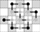
Figure 3: Proving that all lattice-embeddable graphs are bipartite

Fact 2

Any lattice-embeddable graph is bipartite.

[Proof.] Any subgraph of a bipartite graph is bipartite, and the lattice points can be $2$-colored in checkerboard fashion (see Figure 3). ∎

Corollary 3

If a folding of a closed chain (or an open chain with $\mathsf{P}$ endpoints) with $h$ $\mathsf{H}$ nodes has $h$ contacts, then its contact graph is a union of vertex-disjoint even cycles.

[Proof.] In order to achieve $h$ contacts, every $\mathsf{H}$ vertex must have contact degree $2$. ∎

Corollary 4

There can be a contact between two $\mathsf{H}$ nodes only if they have opposite parity (i.e., there is an even number of nodes between them) in the chain.

[Proof.] The path between two nodes on the chain, along with the contact, form a cycle in the folding. Thus the result follows from Fact 2. ∎

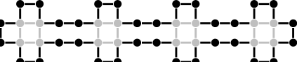
Figure 4: Example of an optimal folding of $({\mathsf{P}}{\mathsf{H}}{\mathsf{P}})^{4k}$.

${\mathsf{H}}{\mathsf{P}}{\mathsf{H}}$	${\mathsf{P}}{\mathsf{H}}{\mathsf{H}}$	${\mathsf{P}}{\mathsf{H}}{\mathsf{P}}{\mathsf{H}}$

Figure 5: Cases for Fact 5, with the forbidden subsequences they imply.

Fact 5

Any optimal folding of the (open or closed) chain $({\mathsf{P}}{\mathsf{H}}{\mathsf{P}})^{4k}$ has a contact graph consisting of $k$ $4$-cycles.

[Proof.] $4k$ contacts are achievable e.g. by a folding analogous to the one shown in Figure 4, and no higher number of contacts is achievable by Fact 1. By Corollary 3 the contact graph is therefore a set of cycles. Now consider some cycle in the contact graph of length greater than 4, and consider the leftmost “_⌜” corner. Up to symmetry, there are three cases, illustrated in Figure 5. In each case there is either a singleton $\mathsf{P}$ or a double $\mathsf{H}$ on the chain. ∎

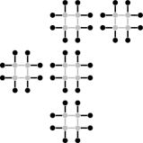
Figure 6: Converting a lattice tree into an optimal embedding of $({\mathsf{P}}{\mathsf{H}}{\mathsf{P}})^{4k}$

Fact 6

For any $n=12k$, there exists an $n$-node (open or closed) chain with at least $2^{\Omega(n)}$ optimal foldings, all with isomorphic contact graphs of size $\Omega(n)$.

[Proof.] We argue that any lattice-embeddable tree on $k$ nodes corresponds to an optimal folding of $({\mathsf{P}}{\mathsf{H}}{\mathsf{P}})^{4k}$. To see this correspondence, take the embedded tree and scale by 4. Replace each node in the tree with a “gadget” consisting of a $4$-cycle from the contact graph, and the associated forced chain edges (see Figure 6). Finally replace the edges of the tree with pairs of edges between adjacent “gadgets”, and close off any remaining ${\mathsf{P}}{\mathsf{P}}$ pairs with chain edges (in the open-chain case, all but one pair is closed off).

Next observe that there are many lattice-embeddable trees on $k$ nodes. A simple exponential lower bound can be obtained by considering the north/east staircase paths; because there are $2$ choices at each step, this gives a lower bound of $2^{k}$. Each tree (folding) is counted at most a constant number times. ∎

The preceeding bound on the number of lattice trees can almost certainly be improved. The number of lattice trees has been studied by the Statistical Physics community, primarily from the point of view of deviation from exponential growth [29, 23, 24]. Based on a combination of theoretical and experimental results it is believed [24] that the number of lattice trees $t_{n}$ with $n$ nodes obeys the following bound

$$t_{n}\in\Omega\left(\frac{3.79^{n}}{n}\right).$$

4 Uniquely Foldable Closed Chains

In this section we are concerned with closed H-P chains whose optimal foldings are unique (modulo isometries). For each $k\geq 1$, we define a closed chain $S_{k}$ as follows. Let $A_{m}$ denote the sequence $({\mathsf{H}}{\mathsf{P}})^{m}$. Define $u=\lceil k/2\rceil$ and $d=\lfloor k/2\rfloor$. Then define $S_{k}$ as ${\mathsf{P}}\,A_{u}\,{\mathsf{P}}\,A_{d}$. Note that $S_{k}$ has exactly two $\mathsf{P}$-$\mathsf{P}$ edges, i.e. edges between two $\mathsf{P}$ nodes. We also define a folding $F_{k}$ of $S_{k}$ as follows (see Figure 7). Let $D_{m}$ (a “down staircase”) denote the alternating path $(\mathsf{E}\mathsf{S})^{m}$. Let $U_{m}$ (an “up staircase”) denote the alternating path $(\mathsf{W}\mathsf{N})^{m}$. If $k$ is even, define $F_{k}$ as $\mathsf{E}\,D_{d}\,\mathsf{W}\,U_{u}$. If $k$ is odd, define $F_{k}$ as $\mathsf{E}\,D_{d}\,\mathsf{S}\,U_{u}$.

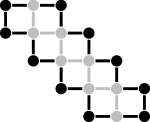
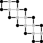
Figure 7: Examples of $S_{k}$ folded according to $F_{k}$ for $k\in\{2,8,9\}$.

The main result of this section is the following theorem.

Theorem 7

For each $k\geq 1$, $F_{k}$ is the unique optimal folding of $S_{k}$.

As well as providing evidence that the H-P model captures some approximation of the mechanism of protein stability for closed chains, Theorem 7 has several less direct consequences. In the next section we will use this theorem to prove a similar result about open chains. Furthermore, Theorem 7 tells us something nonobvious about the shape of optimal foldings in the H-P model, namely that there exist (closed) proteins all of whose optimal foldings are extremely “nonglobular” (noncompact). Along similar lines, in a preliminary version of this paper [2], we conjectured that every closed H-P chain had an optimal folding with the minimum possible area (enclosing no grid points). This conjecture turns out to be false [3].

The conformation graph of an embedding consists of the union of the chain edges and the contact graph. The idea of the proof of Theorem 7 is to show via parity arguments that the conformation graph of any optimal embedding of $S_{j}$ is fixed. Once this is established, the embedding follows from the special form of the conformation graph (all but one face is a $4$-cycle).

Fact 8

There exists a folding of $S_{k}$ with $k-1$ contacts, namely $F_{k}$.

Fact 9

The $\mathsf{H}$ nodes of $S_{k}$ fall into two parity classes, separated into odd and even chains by the two $\mathsf{P}$-$\mathsf{P}$ edges.

In the case of an embedded closed chain $Q$, we distinguish between chordal contacts, i.e. those in the interior of $Q$, and pocket contacts, i.e. those exterior to $Q$.

Lemma 10

There are no pocket contacts in an optimal folding of $S_{k}$.

[Proof.] Each $\mathsf{H}$ node on the bounding box causes at least one missing contact. From Fact 8, we know that an optimal folding can therefore have at most two $\mathsf{H}$ nodes on the bounding box. Because every edge of the chain but two has at least one $\mathsf{H}$ node, and there must be at least one edge on each wall of the bounding box, there must be at least two $\mathsf{H}$ nodes on the bounding box, and this minimum is achievable only if both $\mathsf{P}$-$\mathsf{P}$ edges are on distinct edges of the bounding box. For each $\mathsf{P}$-$\mathsf{P}$ edge construct a slab by extending rays perpendicular to the edge from the endpoints (see Figure 8). In order for a pocket contact to form, one of the odd or even chains must touch or cross one of the slabs. But if any vertex lies on a slab, the corresponding $\mathsf{P}$-$\mathsf{P}$ edge cannot be on the bounding box. ∎

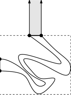
Figure 8: Illustrating the proof of Lemma 10.

Lemma 11

The contact graph is acyclic in any optimal folding of $S_{k}$.

[Proof.] Consider some optimal folding of $S_{k}$. By Lemma 10, we know that all contacts must be chordal. Further observe that the conformation graph must be a planar graph. Consider an arbitrary planar embedding of the chain $S_{k}$. Note that each edge of a contact cycle must go from the odd chain to the even chain or vice-versa. After two steps along a cycle, there is no way to join the first node of the cycle to the (current) last node of the cycle without creating a crossing. ∎

Corollary 12

The contact graph in an optimal folding of $S_{k}$ is a path with $k$ nodes and $k-1$ edges.

[Proof.] This follows from Fact 8 and Lemma 11. ∎

Figure 9: Up to reversal of the labeling, the labeled contact graph of $S_{k}$ is fixed.

Lemma 13

If $k$ is odd, every optimal folding of $S_{k}$ has the same labeled contact graph. If $k$ is even, there are two possible labeled contact graphs and the mapping from one to the other is given by the relabeling $j\mapsto k+1-j$.

[Proof.] Note that the endpoints of the contact path must be adjacent to one of the $\mathsf{P}$-$\mathsf{P}$ edges on the chain because otherwise some $\mathsf{H}$ node would be stranded. Further note that once the starting point of the path is chosen, the rest of the path is determined by an argument similar to the proof of Lemma 11. There is no choice of starting point for the case of $k$ odd, because both endpoints of the contact path must be in the larger parity class of $\mathsf{H}$ nodes. ∎

We can deduce the following from the proof of Lemma 13.

Corollary 14

In the conformation graph of an optimal folding of $S_{k}$,

• There are two $4$-cycles of type ${\mathsf{P}}{\mathsf{P}}{\mathsf{H}}{\mathsf{H}}$,

• There are $(k-2)$ $4$-cycles of type ${\mathsf{P}}{\mathsf{H}}{\mathsf{H}}{\mathsf{H}}$, and

• Each contact edge is contained in exactly two $4$-cycles.

Fact 15

Every $4$-cycle has a unique folding, namely a square.

[Proof.](of Theorem 7) Consider the folded chain as a polygon, decomposed into quadrilaterals by contact edges. From Corollary 14 we can see that the dual graph of the decomposition is itself a path. We construct the folding by following this dual path. We start by choosing an orientation for one of the ${\mathsf{P}}{\mathsf{P}}{\mathsf{H}}{\mathsf{H}}$ $4$-cycles and embedding it. If $k=2$, then we have no choice for the final square. Otherwise, we choose an orientation for the second square and embed it. After the second square, by looking at degrees in the contact graph, it follows that we have no choice in embedding the next $4$-cycle on the dual path. Thus our total choice in embedding was one translation, one rotation, and one reflection. ∎

Corollary 16

For every positive even $n$ there is an $n$-node closed H-P chain with a unique optimal folding.

5 Uniquely Foldable Open Chains

Finally we turn to open H-P chains. Dill et al. [18] computed that for chains of length up to 18, about 2% of chains have unique optimal foldings. In a similar vein, Hayes [22] found that for each $1\leq n\leq 14$ except $3$ and $5$ there is an open chain with a unique optimal folding. We have duplicated the experiments of Dill et al. and extended them to chains of length $20$, with (partial) results given in Table 1. We have further found experimentally that there are H-P chains with unique optimal foldings for lengths 15 through 25. Figure 10 illustrates chains with unique optimal foldings for lengths up to $25$, excluding lengths $2$ (trivial) and $4k$ for $k>3$ (covered by a theorem below). The bias towards ${\mathsf{H}}$ nodes is an artifact of our search program, which enumerates colourings in “binary-counter” order with ${\mathsf{H}}=0$ and ${\mathsf{P}}=1$. It has been reported elsewhere that real proteins have $\mathsf{H}$ to $\mathsf{P}$ ratio of about $2:3$ [25]. We will also see below that in the H-P model, unique optimality is achievable with a ratio very close to $1:1$.

$n$	unique	total	percentage
11	65	2,048	3.174
12	88	4,096	2.148
13	179	8,192	2.185
14	387	16,384	2.362
15	864	32,768	2.637
16	1,547	65,536	2.361
17	3,420	131,072	2.609
18	6,363	262,144	2.427
19	13,486	524,288	2.572
20	24,925	1,048,576	2.377

Table 1: Percentage of H-P chains of length $n$ with unique optimal embeddings.

$$\begin{array}[]{cccc}\includegraphics{oswin4.eps}&\includegraphics{oswin6.eps}&\includegraphics{oswin7.eps}&\includegraphics{oswin8.eps}\\ 4&6&7&8\\[12.91663pt] \includegraphics{oswin9.eps}&\includegraphics{oswin10.eps}&\includegraphics{oswin11.eps}&\includegraphics{oswin12.eps}\\ 9&10&11&12\\[12.91663pt] \includegraphics{oswin13.eps}&\includegraphics{oswin14.eps}&\includegraphics{oswin15.eps}&\includegraphics{oswin17.eps}\\ 13&14&15&17\\[12.91663pt] \includegraphics[scale={0.8}]{oswin18.eps}&\includegraphics[scale={0.8}]{oswin19.eps}&\includegraphics[scale={0.8}]{oswin21.eps}&\includegraphics[scale={0.8}]{oswin22.eps}\\ 18&19&21&22\\[12.91663pt] \includegraphics[scale={0.8}]{oswin23.eps}&&\includegraphics[scale={0.8}]{oswin25.eps}\\ 23&&25\end{array}$$

Figure 10: Examples of H-P chains with unique optimal foldings, shown in their optimal embedding.

A natural question is for what values of $n$ there is an $n$-node open chain with a unique optimal folding. Based on our results about closed chains, one approach is to consider the open version of $S_{k}$ with the first and last nodes removed. That is, define $Z_{k}=({\mathsf{H}}{\mathsf{P}})^{u}({\mathsf{P}}{\mathsf{H}})^{d}$ where $u=\lceil k/2\rceil$ and $d=\lfloor k/2\rfloor$. It turns out that this chain has multiple optimal folding for odd $k$, but only one optimal folding for even $k$ (see Figures 11 and 12).

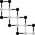
Figure 11: Unique optimal folding of $Z_{8}$.

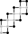
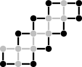
Figure 12: Two optimal foldings for $Z_{9}$.

In what follows, we will establish that up to isometries, the only optimal embedding of $Z_{2k}$ is what we call the standard embedding, namely the $\mathsf{P}$-$\mathsf{P}$ edge horizontal, the two adjacent edges down, the remaining edges on the right alternating right and down, and the remaining edges on the left alternating down and right (the standard embedding of $Z_{8}$ is illustrated in Figure 11). This will establish the following theorem.

Theorem 17

The open chain $Z_{2j}=({\mathsf{H}}{\mathsf{P}})^{j}({\mathsf{P}}{\mathsf{H}})^{j}$ has a unique optimal embedding for each positive $j$.

Combining this theorem with examples illustrated in Figure 10, it turns out that there are open chains with unique optimal foldings for $n=2$, $n=4$, and $6\leq n\leq 25$.

Despite the seeming simplicity of the claim, and the similarity to Theorem 7, the proof of Theorem 17 requires a number of technical lemmas. We will argue that every embedding of $Z_{2k}$ has at least four missing external contacts, and further prove that the standard embedding of $Z_{2k}$ is the only embedding with exactly four missing contacts. We accomplish this by reducing the open-chain case to the closed-chain case discussed in the previous section. In particular, we will show that in an optimal embedding of $Z_{2k}$, the $\mathsf{H}$ endpoints are on the bounding box and in contact. This will allow us to extend any optimal embedding of $Z_{2k}$ to an optimal embedding of $S_{2k}$. The proof can be summarized as follows:

1. An optimal embedding has at most $4$ missing contacts (Fact 18, Corollary 19).

2. An optimal embedding has at least $3$ external missing contacts and at most one internal missing contact (Fact 20, Corollaries 21 and 22).

3. There are no ${\mathsf{H}}$ corners (i.e. turns in the chain) on the bounding box (Lemmas 24 and 25).

4. If an endpoint is on the bounding box, either it is in contact with the other endpoint, or creates an internal missing contact (Lemma 26).

5. In an optimal embedding of $Z_{2k}$, there is at most one ${\mathsf{H}}$ node on the bounding box that is neither a corner, nor an endpoint (Facts 27 and 28, Lemmas 29 and 30).

In the rest of this section, we present the details of the proof of Theorem 17. As in the previous section, we start by observing that any optimal embedding must be at least as good as our example embedding.

Fact 18

The standard embedding of $Z_{2k}$ has only four missing contacts, all external.

Corollary 19

Any optimal embedding of $Z_{2k}$ has at most four missing contacts.

We begin with the following observation.

Fact 20

In any embedding of $Z_{2k}$, either

• Three bounding-box walls contain $\mathsf{H}$ nodes, and one contains only the $\mathsf{P}$-$\mathsf{P}$ edge of $Z_{2k}$, or

• Four bounding-box walls contain $\mathsf{H}$ nodes.

[Proof.] Every bounding-box wall must contain either an edge or an endpoint of $Z_{2k}$. Only one edge of $Z_{2k}$ does not contain an $\mathsf{H}$ node, and each endpoint is a $\mathsf{H}$ node. ∎

Corollary 21

In an optimal embedding of $Z_{2k}$, there are missing external contacts emanating from at least three walls of the bounding box. The fourth wall either contains the $\mathsf{P}$-$\mathsf{P}$ edge, or has a fourth missing external contact.

Corollary 22

Any embedding of $Z_{2k}$ has at least three external missing contacts, and an optimal embedding has at most one internal missing contact.

Fact 23

For $k>1$, the bounding box of any optimal embedding of $Z_{2k}$ has both height and width at least two.

[Proof.] If either dimension of the bounding box is less than 2, then all of the $\mathsf{H}$ nodes are on the bounding box. ∎

Fact 20 implies that there is at least one nonendpoint $\mathsf{H}$ node $v$ on the bounding box. We break this down into two cases. Two edges adjacent to $v$ could be on the bounding box, in which case we call $v$ a straight $\mathsf{H}$ node. Alternatively, only one edge adjacent to $v$ could be on the bounding box, in which case we call $v$ an $\mathsf{H}$ corner. We first argue that in an optimal embedding of $Z_{2k}$ there are no $\mathsf{H}$ corners at the corner of the bounding box.

Lemma 24

In an optimal embedding of $Z_{2k}$, there are no $\mathsf{H}$ corners at the corner of the bounding box.

[Proof.] Let $v$ be an $\mathsf{H}$ corner which is also on the northeast corner of the bounding box. We distinguish three cases, as illustrated in Figure 13. In the first case, $v$ is not adjacent to the $\mathsf{P}$-$\mathsf{P}$ edge. In the second, $v$ is adjacent to the $\mathsf{P}$-$\mathsf{P}$ edge but not on the same wall of the bounding box. In the third, $v$ is adjacent to the $\mathsf{P}$-$\mathsf{P}$ edge and on the same wall of the bounding box.

Figure 13: Illustrating the proof of Lemma 24.

We first consider the case where $v$ is not adjacent to the $\mathsf{P}$-$\mathsf{P}$ edge. Because the two $\mathsf{H}$ nodes nearest $v$ (two edges away) cannot both occupy the lattice point southwest from $v$, one of these two nodes must also be on the bounding box. Suppose there exists an $\mathsf{H}$ node on the bounding box two edges south from $v$, and consider the position of the other node $u$ (refer to Figure 13). If $u$ is on the bounding box then there exists a fourth external missing contact along only two walls (north and east) of the bounding box. This implies the presence of a fifth external missing contact. Thus the embedding is not optimal by Corollary 19. The other possibility is that the path from $v$ to $u$ is west-south, but this creates a missing internal contact between $u$ and a $\mathsf{P}$ node. Because the presence of a fourth external contact is necessary, this embedding cannot be optimal.

We next consider the case where $v$ is adjacent to the $\mathsf{P}$-$\mathsf{P}$ edge, but where the $\mathsf{P}$-$\mathsf{P}$ edge is not on the same bounding box wall as $v$ (refer to Figure 13). This implies that the $\mathsf{P}$-$\mathsf{P}$ edge occupies the lattice point southwest from $v$, and therefore there exists an $\mathsf{H}$ node two edges south from $v$. Because the east wall has two external missing contacts and the $\mathsf{P}$-$\mathsf{P}$ edge cannot be on the south wall, by Corollary 21 the $\mathsf{P}$-$\mathsf{P}$ edge must be on the west wall of the bounding box (otherwise, there would be external missing contacts on each wall, for a total of five, and the embedding would not be optimal). By Fact 23, this is a contradiction.

Finally, we consider the case where $v$ is adjacent to the $\mathsf{P}$-$\mathsf{P}$ edge and on the same wall (see Figure 13). We assume that the $\mathsf{P}$-$\mathsf{P}$ edge lies directly south of $v$. Because the north and east walls have two external missing contacts and the $\mathsf{P}$-$\mathsf{P}$ edge, any additional external missing contact on these walls would imply suboptimality by Corollary 21. Therefore the two $\mathsf{H}$ nodes nearest $v$ cannot lie on either of these walls, and must lie as indicated in the figure. This causes an internal missing contact between an $\mathsf{H}$ node and a $\mathsf{P}$ node. Thus there are at least five missing contacts, and the embedding is not optimal. ∎

We now expand the restriction on $\mathsf{H}$ corners to include the entire bounding-box wall.

Lemma 25

There are no $\mathsf{H}$ corners on the bounding box in an optimal embedding of $Z_{2k}$.

[Proof.] By Lemma 24, we need only consider the case of an $\mathsf{H}$ corner in the relative interior of a bounding box edge. Let $v$ be such an $\mathsf{H}$ corner. We assume that the edges of the chain adjacent to $v$ are to the west and the south. We distinguish two cases, as illustrated in Figure 14. In the first case, $v$ has no contacts and thus has a missing external contact and a missing internal contact (along the wall of the bounding box). In the second case, $v$ has an internal contact, which must be with a second $\mathsf{H}$ corner or an endpoint.

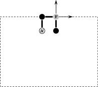
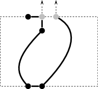
Figure 14: Illustrating the proof of Lemma 25.

We first consider the case where $v$ has no contacts. Because there is a missing internal contact, there can only be three external missing contacts if the embedding is to be optimal. Therefore the $\mathsf{P}$-$\mathsf{P}$ edge must be on the bounding box, and cannot be on the north wall. Furthermore, no other $\mathsf{H}$ node can be on the north wall. Consider the edge adjacent to $v$ on the north wall, and the node $u$ which follows it. Because $u$ cannot be on the north wall, its only possible position is south west of $v$. This creates a second internal missing contact between $u$ and a $\mathsf{P}$ node (if $u$ is an $\mathsf{H}$ node) or an extra external missing contact (if $u$ is part of the $\mathsf{P}$-$\mathsf{P}$ edge), causing suboptimality.

We finally consider the case where $v$ has an internal contact, which must be with a second $\mathsf{H}$ corner or endpoint $w$. Because $w$ has a second external missing contact on the north wall, the $\mathsf{P}$-$\mathsf{P}$ edge must lie on the bounding box by Corollary 21. Furthermore, the $\mathsf{P}$-$\mathsf{P}$ edge must lie on the path from $v$ to $w$ because $v$ and $w$ have different parity. Thus the path from $v$ to the $\mathsf{P}$-$\mathsf{P}$ edge creates a barrier between all points west of this path and all points after the $\mathsf{P}$-$\mathsf{P}$ edge. The endpoint of the same parity as $v$ must lie west of the path, as the chain cannot go outside the bounding box. This endpoint has three missing contacts, for a total of five for the chain. Therefore the embedding is not optimal. ∎

We have now established that if an $\mathsf{H}$ node is on the bounding box, it must either be straight or an endpoint. With respect to endpoints, we observe the following:

Lemma 26

In an optimal embedding of $Z_{2k}$, if an endpoint is on the bounding box, then either there is an internal missing contact, or the two endpoints are in contact.

[Proof.] An endpoint has three potential contacts; at least one of which lies along the wall of the bounding box. Either this is an internal missing contact, or the endpoint is adjacent to an $\mathsf{H}$ node. Because there are no $\mathsf{H}$ corners in an optimal embedding, this $\mathsf{H}$ node must be the second endpoint. ∎

Because there are only two endpoints and one $\mathsf{P}$-$\mathsf{P}$ edge, we know there must be at least one straight $\mathsf{H}$ node on the bounding box. We define two kinds of straight $\mathsf{H}$ nodes. We say a straight $\mathsf{H}$ node $v$ is coupled if the preceding or following $\mathsf{H}$ node is also on the same wall of the bounding box as $v$; otherwise it is solitary. These cases are illustrated in Figure 15.

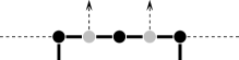
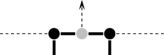
Figure 15: A pair of coupled straight $\mathsf{H}$ nodes, and a solitary straight $\mathsf{H}$ node.

Figure 16: Illustrating the proof of Fact 27.

Fact 27

In an optimal embedding of $Z_{2k}$, a solitary straight $\mathsf{H}$ node must either be adjacent to the $\mathsf{P}$-$\mathsf{P}$ edge or contact with an endpoint.

[Proof.] Let $v$ be a solitary straight $\mathsf{H}$ node on the north wall of the bounding box which is not adjacent to the $\mathsf{P}$-$\mathsf{P}$ edge. Then there must be two $\mathsf{H}$ nodes immediately southwest and southeast of $v$, as illustrated in Figure 16. The lattice point south of $v$ cannot be the adjacent $\mathsf{P}$ node of any of the $\mathsf{H}$ nodes, nor can it be vacant, because there would be at least two missing internal contacts, violating optimality. ∎

Fact 28

In an optimal embedding of $Z_{2k}$, there is at most one pair of coupled straight $\mathsf{H}$ nodes.

[Proof.] Each $m$-tuple of coupled $\mathsf{H}$ nodes causes $m$ external missing contacts on the same bounding box wall. There can be at most one wall with two external missing contacts, and none with three or more. ∎

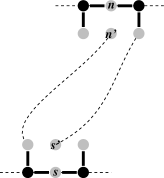
Figure 17: Illustrating the proof of Lemma 29.

The following two lemmas establish that there is at most one solitary straight $\mathsf{H}$ node.

Lemma 29

In an optimal embedding of $Z_{2k}$, there is at most one solitary straight $\mathsf{H}$ node in contact with an endpoint.

[Proof.] Assume there are two such straight $\mathsf{H}$ nodes, $n$ and $s$, which contact with two endpoints, $n^{\prime}$ and $s^{\prime}$, respectively. We assume $n$ is on the north wall and $s$ on the south; the argument can be slightly modified for any other case. Because $n^{\prime}$ and $s^{\prime}$ are of different parity, so too must be $n$ and $s$. Therefore there is a path on the chain from $n$ to $s^{\prime}$ which does not pass through $s$, and a path from $s$ to $n^{\prime}$ which does not pass through $n$. Assume without loss of generality that the path from $n$ to $s^{\prime}$ leaves $n$ to the east, as in Figure 17. Then the path from $s$ to $n^{\prime}$ must leave $s$ to the west to avoid intersection. Because the chain is connected, there must be a path from $n$ to $s$. The only possibility left is that the path leaves $n$ to the west, and enters $s$ from the east. However, this requires the path to either leave the bounding box, or intersect the rest of the chain, neither of which is possible. ∎

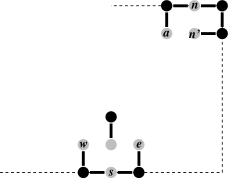
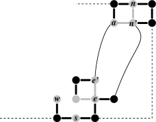
Figure 18: Illustrating the proof of Lemma 30.

Lemma 30

In an optimal embedding of $Z_{2k}$, there is at most one solitary straight $\mathsf{H}$ node on the bounding box.

[Proof.] Suppose there is more than one straight $\mathsf{H}$ node on the bounding box. By Fact 27 and Lemma 29 there must be exactly two: one must be adjacent to the $\mathsf{P}$-$\mathsf{P}$ edge; the other must contact with an endpoint. We observe that the $\mathsf{P}$-$\mathsf{P}$ edge must be on the bounding box, because each wall not containing a solitary $\mathsf{H}$ node must otherwise contain either a pair of coupled straight $\mathsf{H}$ nodes or an endpoint; any combination of these two possibilities leads to a total of at least $5$ missing contacts (apply Lemma 26 in the case of an endpoint).

Assume the north, east, and south walls are covered by the two solitary straight $\mathsf{H}$ nodes and the $\mathsf{P}$-$\mathsf{P}$ edge. We assume the configuration in Figure 18 without loss of generality (the argument here will not depend on whether the two solitary nodes are on opposite walls of the bounding box). Call the $\mathsf{H}$ node on the south wall $s$, and the $\mathsf{H}$ nodes preceding and following (northeast and northwest of $s$) $e$ and $w$. One endpoint of the chain is in contact with $e$, $w$, and $s$.

Consider the possibilities for covering the west wall of the bounding box: there is either a pair of coupled straight nodes, or an endpoint. By Lemma 26, either case results in two missing contacts, both either contained in or emanating from the west wall. It follows that we need only find one more missing contact to establish suboptimality.

Consider the $\mathsf{H}$ node $e$ east of $s$; $e$ cannot be on the bounding box as this would create an external missing contact. Placing an $\mathsf{H}$ node east of $e$ just creates another internal missing contact, which in turn cannot be blocked without creating a missing contact with the $\mathsf{P}$ node between $s$ and $e$ on the chain. It follows that the chain must turn east at $e$; in order to avoid an internal missing contact, there must be an ${\mathsf{H}}$ node north of $e$ (at $e^{\prime}$ in Figure 18), and a chain edge west from this ${\mathsf{H}}$ node. Note that lattice point north of $w$ (i.e. $w^{\prime}$) cannot contain an $\mathsf{H}$ node, as this would create an internal missing contact.

By planarity, the subchains containing $e$ and $e^{\prime}$ must be connected to the $\mathsf{P}$-$\mathsf{P}$ edge as shown in Figure 18. Consider the polygon $Q$ formed these connecting chains, along with the contacts $ee^{\prime}$ and $an^{\prime}$. By an argument similar to Lemma 11 (with the extension that no contacts can be formed with $w$), all of the remaining contacts for $\mathsf{H}$ nodes on this polygon must be internal to $Q$. Because there is an imbalance in the parity of potential contacts for nodes on $Q$, this forces an internal missing contact. ∎

We are finally ready to characterize the intersection of an optimal embedding of $Z_{2k}$ with its bounding box.

Lemma 31

In an optimal embedding of $Z_{2k}$, the two endpoints are on the bounding box and in contact, and the $\mathsf{P}$-$\mathsf{P}$ edge is adjacent to a solitary $\mathsf{H}$ node, both of which are also on the bounding box. Furthermore, there are no internal missing contacts.

[Proof.] By Lemma 30 there is at most one solitary straight $\mathsf{H}$ node on the bounding box, and there is of course only one $\mathsf{P}$-$\mathsf{P}$ edge. On the other two walls of the bounding box, there are either two endpoints, or one endpoint and one pair of coupled straight $\mathsf{H}$ nodes. In the last case, the endpoint causes one internal missing contact by Lemma 26, and the coupled straight $\mathsf{H}$ nodes cause two external missing contacts. Therefore there are no coupled straight $\mathsf{H}$ nodes. Furthermore, because both endpoints are on the bounding box, they must be in contact by Lemma 26 to avoid having two internal missing contacts. Because the two endpoints contact, and are both on the bounding box, they have two external missing contacts on the same wall. Therefore there are four external missing contacts in an optimal embedding, and thus no internal missing contacts. ∎

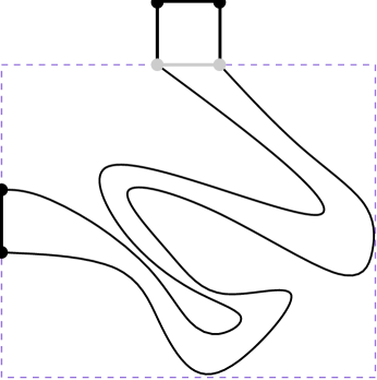
Figure 19: Converting an optimal embedding of $Z_{2k}$ into an optimal embedding into an optimal embedding of $S_{2k}$.

The previous lemma claims in essence that the open chain $Z_{2k}$ behaves just like a closed chain in any optimal embedding. We formalize this intuition as follows:

Theorem 32

There are as many optimal embeddings of $S_{2k}$ as there are of $Z_{2k}$.

[Proof.] By the preceding lemma, in an optimal embedding the endpoints $Z_{2k}$ are in contact and on the bounding box; thus we can convert an optimal embedding of $Z_{2k}$ into an optimal embedding of $S_{2k}$ by adding a second $\mathsf{P}$-$\mathsf{P}$ edge, outside the bounding box (see Figure 19). ∎ Theorem 17 is a straightforward consequence of the preceding theorem and Theorem 7.

We expect that by similar methods we can prove the following:

Conjecture 33

For odd $k\geq 5$, the open chain $Z_{k}$ has exactly two optimal embeddings.

We have computationally verified this conjecture for chains of length up to $26$, that is, for odd $5\leq k\leq 13$. For $k=1$ and $k=3$, $Z_{k}$ in fact has a unique optimal folding.

6 Conclusions and Directions for Future Work

In this paper we considered a natural characterization of stable protein folding in the 2D H-P model, namely uniqueness of optimal folding. We established that

1. There exist closed H-P chains with unique optimal folds for all (even) lengths, and

2. There exist open H-P chains with unique optimal folds for all lengths divisible by $4$.

We further observed that

1. There exist arbitrarily long H-P chains with linear sized contact graphs and an exponential number of optimal foldings.

There are several natural directions for future work, involving more general lattices, asymptotic bounds, and algorithmic questions, as summarized below.

There is a great deal of natural skepticism about the biological relevance of results stemming from the 2D square lattice. While certain qualitative properties are independant of the lattice used [18], in the case of the present work it seems clear that the bipartiteness of the lattice plays an important (and difficult-to-motivate) role. It is thus important to consider nonsquare lattices in 2D, and preferably nonbipartite lattices in 3D. Examples include the triangular lattice in 2D, and the face-centered cubic (FCC) lattice suggested by Neumaier [31] as a minimal approximation of chemical bond distances and angles. For example, Agarwala et al. [1] consider both of these lattices.

The existence of H-P chains with unique embeddings in a given lattice is only a first step to understanding the behaviour of these models with respect to uniqueness. Experimental results [18] have shown that about $2\%$ of open chains up to length $18$ have unique optimal foldings. It would be very nice to have asymptotic bounds for the fraction of H-P chains with unique optimal foldings. Rather than considering arbitrary H-P chains, it would also be useful to see what fraction of the proteins in the Protein Data Bank [10] fold uniquely in the H-P model. It is likely that the best that can be hoped for is that real proteins have a small number of optimal foldings.

From a sequence-design point of view, the more interesting question is not whether there exists an H-P sequence with a small number of optimal foldings, but how to design sequences with this property. From a combinatorial point of view, this asks for a characterization of what sequences have unique (or a small number of) optimal foldings.

From an algorithmic point of view, there are two natural questions. The first problem is whether there is an efficient algorithm to recognize sequences with unique optimal foldings. The second prolem is whether the problem of finding a minimum energy folding of an H-P chain is still NP-hard when restricted to chains with unique optimal foldings.

Finally, there may be better definitions of folding stability in the H-P model. We have mentioned the notion of a large gap in the number of contacts between the optimal folding and the next best folding [37, 38]. Given that the H-P model is only approximate, it may also be inappropriate to distinguish between chains having e.g. 1 and 2 optimal embeddings.

References

- [1] R. Agarwala, S. Batzoglou, V. Dancik, S. E. Decatur, M. Farach, S. Hannenhalli, S. Muthukrishnan, and S. Skiena. Local rules for protein folding on a triangular lattice and generalized hydrophobicity in the HP model. Journal of Computational Biology, 4(2):275–296, 1997.
- [2] O. Aichholzer, D. Bremner, E. D. Demaine, H. Meijer, V. Sacristán, and M. Soss. Long proteins with unique optimal foldings in the H-P model. In 17th European Workshop on Computational Geometry, Mar. 2001.
- [3] G. Aloupis, E. D. Demaine, P. Morin, and M. Soss. On the area of minimum energy foldings of H-P chains. Manuscript, Feb. 2001.
- [4] C. Anfinsen. Studies on the principles that govern the folding of protein chains. In Les Prix Nobel en 1972, pages 103–119. Nobel Foundation, 1972.
- [5] R. Backofen. Constraint techniques for solving the protein structure prediction problem. In Proceedings of the 4th International Conference on Principles and Practice of Constraint Programming, volume 1520 of Lecture Notes in Computer Science, pages 72–86, October 1998.
- [6] R. Backofen. Using constraint programming for lattice protein folding. In Proceedings of the 3rd Pacific Symposium on Biocomputing, pages 387–398, January 1998.
- [7] R. Backofen. An upper bound for number of contacts in the HP-model on the face-centered-cubic lattice (FCC). In Proceedings of the 11th Annual Symposium on Combinatorial Pattern Matching, volume 1848 of Lecture Notes in Computer Science, pages 277–292, Montréal, 2000.
- [8] R. Backofen and S. Will. Optimally compact finite sphere packings — hydrophobic cores in the FCC. In Proceedings of the 12th Annual Symposium on Combinatorial Pattern Matching, volume 2089 of Lecture Notes in Computer Science, pages 257–271, Jerusalem, July 2001.
- [9] B. Berger and T. Leighton. Protein folding in the hydrophobic-hydrophilic (HP) model is NP-complete. Journal of Computational Biology, 5(1):27–40, 1998.
- [10] H. M. Berman, J. Westbrook, Z. Feng, G. Gilliland, T. N. Bhat, H.Weissig, I. N. Shindyalov, and P. E. Bourne. The protein data bank. Nucleic Acids Research, 28:235–242, 2000.
- [11] E. Bornberg-Bauer. Chain growth algorithms for HP-type lattice proteins. In Proceedings of the 1st Annual International Conference on Computational Molecular Biology, pages 47–55, 1997.
- [12] H. S. Chan and K. A. Dill. Origins of structure in globular proteins. Proceedings of the National Academy of Sciences USA, 87:6388–6392, August 1990.
- [13] H. S. Chan and K. A. Dill. Polymer principles in protein structure and stability. Annual Reviews of Biophysics and Biophysical Chemistry, 20:447–490, 1991.
- [14] H. S. Chan and K. A. Dill. The protein folding problem. Physics Today, pages 24–32, February 1993.
- [15] P. Clote and R. Backofen. Computational Molecular Biology: an Introduction, chapter 6. Wiley Series in Mathematical and Computational Biology. John Wiley and Sons Ltd., 2000.
- [16] P. Crescenzi, D. Goldman, C. Papadimitriou, A. Piccolboni, and M. Yannakakis. On the complexity of protein folding. Journal of Computational Biology, 5(3), 1998.
- [17] K. A. Dill. Dominant forces in protein folding. Biochemistry, 29(31):7133–7155, August 1990.
- [18] K. A. Dill, S. Bromberg, K. Yue, K. N. Fiebig, D. P. Yee, P. D. Thomas, and H. S. Chan. Principles of protein folding — A perspective from simple exact models. Protein Science, 4:561–602, 1995.
- [19] K. A. Dill, K. M. Fiebig, and H. S. Chan. Cooperativity in protein-folding kinetics. Proceedings of the National Academy of Sciences USA, 90(5):1942–1946, March 1993.
- [20] C. Floudas and P. Pardalos, editors. Optimization in Computational Chemistry and Molecular Biology, volume 40 of Nonconvex Optimization and its Applications. Kluwer Scientific, 2000.
- [21] W. E. Hart and S. Istrail. Fast protein folding in the hydrophobic-hydrophilic model within three-eights of optimal. In Proceedings of the 27th Annual ACM Symposium on the Theory of Computing, pages 157–168, Las Vegas, Nevada, May–June 1995.
- [22] B. Hayes. Prototeins. American Scientist, 86:216–221, 1998.
- [23] E. J. Janse Van Rensburg. On the number of trees in . Journal of Physics A, 25:3523–3528, 1992.
- [24] I. Jensen. Enumerations of lattice animals and trees. Journal of Statistical Physics, 102(3–4):865–881, Feb. 2001.
- [25] J. M. Kleinberg. Efficient algorithms for protein sequence design and the analysis of certain evolutionary fitness landscapes. In Proceedings of the 3rd International Conference on Computational Molecular Biology, pages 226–236, Lyon France, 1999. ACM.
- [26] K. F. Lau and K. A. Dill. A lattice statistical mechanics model of the conformation and sequence spaces of proteins. Macromolecules, 22:3986–3997, 1989.
- [27] K. F. Lau and K. A. Dill. Theory for protein mutability and biogenesis. Proceedings of the National Academy of Sciences USA, 87:638–642, January 1990.
- [28] D. J. Lipman and W. J. Wilber. Modelling neutral and selective evolution of protein folding. Proceedings of The Royal Society of London, Series B, 245(1312):7–11, 1991.
- [29] N. Madras and G. Slade. The Self-Avoiding Walk. Birkhäuser, 1996.
- [30] K. M. Merz and S. M. Le Grand, editors. The Protein Folding Problem and Tertiary Structure Prediction. Birkhäuser, Boston, 1994.
- [31] A. Neumaier. Molecular modeling of proteins and mathematical prediction of protein structure. SIAM Review, 39(3):407–460, 1997.
- [32] A. Newman. A new algorithm for protein folding in the HP model. In Proceedings of the 13th Annual ACM-SIAM Symposium on Discrete Algorithms, pages 876–884, San Francisco, January 2002.
- [33] G. Song and N. Amato. Using motion planning to study protein folding pathways. In Proceedings of the 5th International Conference on Computational Molecular Biology, pages 287–296. ACM, 2001.
- [34] R. Unger and J. Moult. Finding the lowest free energy conformation of a protein is a NP-hard problem: Proof and implications. Bulletin of Mathematical Biology, 55(6):1183–1198, 1993.
- [35] R. Unger and J. Moult. A genetic algorithm for 3D protein folding simulations. In Proceedings of the 5th International Conference on Genetic Algorithms, pages 581–588, San Mateo, CA, 1993.
- [36] R. Unger and J. Moult. Genetic algorithms for protein folding simulations. Journal of Molecular Biology, 231(1):75–81, 1993.
- [37] A. Šali, E. Shaknovich, and M. Karplus. How does a protein fold. Nature, 369:248–251, 1994.
- [38] A. Šali, E. Shaknovich, and M. Karplus. Kinetics of protein folding: A lattice model study of the requirements for folding to the native state. Journal of Molecular Biology, 235:1614–1636, 1994.