The Dynamics of AdaBoost Weights
Tells You What’s Hard to Classify

Abstract

The dynamical evolution of weights in the AdaBoost algorithm contains useful information about the rôle that the associated data points play in the built of the AdaBoost model. In particular, the dynamics induces a bipartition of the data set into two (easy/hard) classes. Easy points are ininfluential in the making of the model, while the varying relevance of hard points can be gauged in terms of an entropy value associated to their evolution. Smooth approximations of entropy highlight regions where classification is most uncertain. Promising results are obtained when methods proposed are applied in the Optimal Sampling framework.

1 Introduction

In this paper we investigate the boosting weight dynamics induced by classification procedures of the AdaBoost family [2, 8], and show how it can be exploited to for highlighting points and regions of uncertain classification. Friedman et al. [3] proposed to analyze and trim the distribution of weights over a training sample in order to reduce computation without sacrificing accuracy. Here, we focus instead on tracking the dynamics of the boosting weight of individual points. By introducing the notion of entropy of the weight evolution, we can clarify the notions of “easy” and the “hard” points as the two types of weight dynamics being observed: in particular, in different classification tasks and with different base models it is found that a group of points may be selected which have very low (ideally, zero) entropy of weight evolution: the easy points. In this framework, we can answer questions as: do easy point play any role in building the AdaBoost model? For hard points, can different degrees of “hardness” be identified which account for different degrees of classification uncertainty? Do easy/hard points show any preference about where to concentrate? The first two questions are clearly connected to equivalent results in the framework of Support Vector Machines: in a number of experiments, hard points are found indeed mostly nearby the classification boundary. In the second part of this paper, the smooth approximation (by kernel regression) of the weight entropy at training data is proposed as an indicator function of classification uncertainty, thereby obtaining a region highlighting methodology. As a natural application, a strategy for optimal sampling in classification tasks was implemented: compared with uniform random sampling, the entropy-based strategy is clearly more effective. Moreover, it compares favorably with an alternative margin-based sampling strategy.

2 The Dynamics of Weights

In the present section, the dynamics that the AdaBoost algorithm sets over the weights is singled out for study. In particular, the intuition is substantiated that the evolution of weights yields information about the varying relevance that different data points have in the built of the AdaBoost model.

Let $D\equiv\{{\bf x}_{i},y_{i}\}_{i=1}^{N}$ be a two-class set of data points, where the ${\bf x}_{i}$s belong to a suitable region, $X$, of some (metric) feature space, and $y_{i}$ takes values in $\{1,-1\}$, for $1\leq i\leq N$. The AdaBoost algorithm iteratively builds a class membership estimator over $X$ as a thresholded linear superposition of different realizations, $M_{k}$, of a same base model, $M$. Any model instance, $M_{k}$, resulting from training at step $k$ depends on the values taken at the same step by a set of $N$ numbers (in the following, the weights), ${\bf w}=w_{1},\dots w_{N}$ – one for each data point. After training, weights are updated: those associated to points misclassified by the current model instance are increased, while decreased are those for which the associated point is classified correctly. An interesting variant of this basic scheme consists in training the different realizations of the base model, not on the whole data set, but on Bootstrap replicates of it [6]. In this second scheme, samplings are extracted according to the discrete probability distribution defined by the weights associated to data points, normalized to sum one.

In Fig. 1a the plots are reported of the evolution of the weights associated to 3 data points when the AdaBoost algorithm is applied to a simple binary classification task on synthetic two-dimensional data (experiment A-Gaussians as described in Sec. A.1). Except for occasional bursts, the weight associated to the first point goes rapidly to zero, while the weights associated to the second and third point keep on going up and down in a seemingly chaotic fashion. Our experience is that these two types of behaviour are not specific of the case under consideration, but can be observed in any AdaBoost experiment. Moreover, tertium non datur, i.e., no other qualitative behaviour is observed (as, for example, that some weight tends to a strictly positive value).

2.1 Easy Vs. Hard Data Points

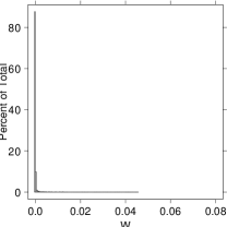
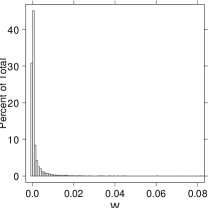
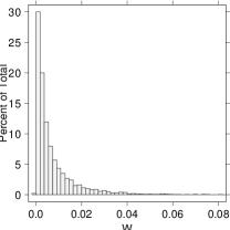
(a) (b)

Figure 1: Evolution of weights in the AdaBoost algorithm. (a) The evolutions over 5000 steps of the AdaBoost algorithm are reported for the weights associated to 3 data points of experiment A-Gaussians. From left to right: an “easy” data point (the weight tends to zero), and two “hard” data points (the weight follows a seemingly random pattern). (b) The corresponding frequency histograms.

The hypothesis therefore emerges that the AdaBoost algorithm set a partition of data points into two classes: on one side the points whose weight tends rapidly to zero; on the other, the points whose weight show an apparently chaotic behaviour. In fact, the hypothesis is perfectly consistent with the rationale underlying the AdaBoost algorithm: weights associated to those data points that several model instances classify correctly even when they are not contained in the training sample follow the first kind of behaviour. In practice independently of which bootstrap sample is extracted, these points are classified correctly, and their weight is consequently decreased and decreased. We call them the “easy” points. The second type of behaviour is followed by the points that, when not contained in the training set, happen to be often misclassified. A series of misclassifications makes the weight associated with any such point increase, thereby increasing the probability for the point to be contained in the following bootstrap sample. As the probability increases and the point is finally extracted (and classified correctly), its weight is decreased; this in turn makes the point less likely to be extracted – and so forth. We call this kind of points “hard”.

In Fig. 1b, histograms are reported of the values that the weights associated to the same 3 data points of Fig. 1a take over the same 5000 iterations of the AdaBoost algorithm. As expected, the histogram of (easy) point 1 is very much squeezed towards zero (more than 80% of weights lies below $10^{-6}$). Histograms of (hard) points 2 and 3 exhibit the same Gamma-like shape, but differ remarkably for what concerns average and dispersion. Naturally, the first question is whether any limit exists for these distributions. For each data point, two unbinned cumulative distributions were therefore built by taking the weights generated by the first 3000 steps of the AdaBoost algorithm, and those generated over the whole 5000 steps. The same-distribution hypothesis was then tested by means of the Kolmogorov-Smirnov (KS) test [5]. Results are reported in Fig. 2a, where $p$-values are plotted against the mean value of all 5000 values. It is interesting to notice that for mean values close to 0 (easy points) the same-distribution hypothesis is always rejected, while it is typically not-rejected for higher values (hard points). It seems that easy points may be confidently identified by simply considering the average of their weight distribution. A binary LDA classifier was therefore trained on the data of Fig. 2a. By setting a $p$-value threshold equal to 0.05, the resulting precision (the complement to 1 of the fraction of false negative) was equal to 0.79 and recall (the complement to 1 of the fraction of false positive) was equal to 0.96.

2.2 Entropy

Can we do any better at separating easy points from hard ones? For hard points, can different degrees of “hardness” be identified which account for different degrees of classification uncertainty? What we are going to show is that by associating a notion of entropy to the evolutions of weights both questions can be answered in the positive. To this end, the interval $[0,1]$ is partitioned into $L$ subintervals of length $1/L$, and the entropy value is computed as $\sum_{i=1}^{L}f_{i}~{}log_{2}~{}f_{i}$, where $f_{i}$ is the relative frequency of weight values falling in the $i$-th subinterval ($0~{}log_{2}~{}0$ is set to $0$). For our cases, $L$ was set to 1000.

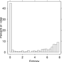
(a) (b) (c)

Figure 2: Separating easy form hard points. (a) $p$-values of the KS test Vs. mean values of frequency histograms. (b) $p$-values of the KS test Vs. entropy of frequency histograms. As in (a), the horizontal line marks the threshold value for the LDA classifier. (c) Histogram of entropy values for the 400 data points of experiment A-Gaussians.

Qualitatively, the relationship between entropy and $p$-values of the KS test is similar to the one holding for the mean (Fig. 2a-b). Quantitatively, however, a difference is observed, since the LDA classifier trained on these data performs much better in precision and slightly worse in recall (respectively, 0.99 and 0.90, as compared to 0.79 and 0.96). This implies that the class of easy points can be identified with higher confidence by using the entropy in place of the mean value of the distribution. Further support to the hypothesis of a bipartite (easy/hard) nature of data points is gained by observing the frequency histogram of entropies for the 400 points of experiment A-Gaussians (Fig. 2c), from which two groups of data points emerge as clearly separated. The first is the zero entropy group of easy points, and the second is the group of hard points.

Do easy/hard points show any preference about where to concentrate? In Fig. 3a hard and easy points are shown as determined for the experiment A-Sin (see Sec. A.1 for details). Hard points are mostly found nearby the two-class boundary; yet, their density is much lower along the straight segment of the boundary (where the boundary is smoother), and appear therefore to concentrate where the classification uncertainty is highest. Easy points to the opposite. Considering that easy points stay well clear of the boundary (i.e., hard points typically interpose between them and the boundary), what one may then question is whether they play any rôle in the built of the AdaBoost model. The answer is no. In fact, the models built disregarding the easy points are practically the same as the models built on the complete data set. In the experiment of Fig. 3 only the $0.55\%$ of $10000$ test points were classified differently by the two models, as contrasted to reduction of the training set from $400$ to only $111$ (hard) points.

2.3 Smoothing the Entropy

In the previous section, the entropy of the weight frequency histogram was introduced as an indicator of the uncertainty of classifying the associated data point as belonging to class $-1$ or $1$. By defining a smooth approximation to the punctual entropy values associated to data points, we now extend the notion of classification uncertainty to the whole domain of our binary classifier. For simplicity sake, kernel regression was employed – i.e., the entropy values at data points are convolved with a Gaussian kernel of fixed bandwidth [9]. In so doing, a scalar entropy function, $H=H({\bf x})$, is defined on $A$. In Fig. 3b, the grey levels encode the values of $H$ (increasing from black to white) for the experiment A-Sin.

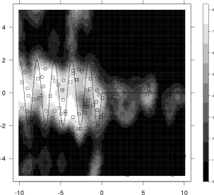
(a) (b)

Figure 3: (a) Easy (white) and hard (black) data points of experiment A-Sin obtained by thresholding the histogram of entropy. Squares and circlets express the class. (b) Level-plot of the $H$ function. Grey levels encode $H$ values (see scale on the right).

The method appears capable of highlighting regions where classification turns out uncertain – due to the distribution of data points, the morphology of the class boundary or both. Of course, function $H$ depends on the geometric properties specific of the base model adopted, and its degree of smoothness depends on the size of the convolution kernel. It should be noticed, however, that the bias/variance balance can be controlled by suitably tuning the convolution parameters. Finally, more sophisticated local smoothing techniques may be employed as well (e.g., Radial Basis Functions) which may adapt to directionality, known morphology of the boundary or local density of sample points.

3 An Application to Optimal Sampling

To illustrate the applicability of notions developed above to practical cases, we refer to the framework of optimal sampling [1]. In general, an optimal sampling problem is one in which a cost is associated to the acquisition of data points, in such a way that solving the problem consists not only in minimizing the classification (or regression) error but also in keeping the sampling cost as low as possible. A typical setting for this class of problems is the one in which we start from an assigned set of (sparse) data points, and we then incrementally add points to the training set on the basis of certain information extracted from intermediate results.

(a) (b)

Figure 4: Misclassification error as a function of the number of training points for the entropy based scheme is compared to the uniform random sampling and the margin sampling strategy. (a) Experiment B-Sin. (b) Experiment B-Spiral.

For the experiments reported below, which are based on the same settings as Sin and Spiral of Sec. A.1 (see also Sec. A.2 for details), we started from a small set of sparse two-dimensional binary classification data. High-uncertainty areas are identified by means of the method described in Sec. 2.3, and additional training points are chosen in these areas. Assuming a unitary cost for each new point, performance of the procedure is finally evaluated by analyzing the sampling cost against the classification error.

In Fig. 4, two plots are reported of the classification error as function of the number of training points. Comparison is made with a blind (randomly uniform) sampling strategy, and with a specialization of uncertainty sampling strategy as recently proposed in [4]. The latter consists in adding training points where the classifier is less certain of class membership. In particular, the classifier was the AdaBoost model and the uncertainty indicator was the margin of the prediction.

Results reported in Fig. 4 show that in both experiments the entropy sampling method holds a definite advantage on the random sampling strategy. In the first experiment, an initial advantage of entropy over the margin based sampling is also observed, but the margin strategy takes over as the number of samplings goes beyond 400. It should be noticed, however, that the margin sampling automatically adapts its spatial scale to the increased density of sampling points, while our entropy method does not (the size of the convolution kernel is fixed). In fact, in the experiment B-Spiral (Fig. 4b) where the boundary has a more complex structure, (and the size of convolution kernel smaller), 1000 samplings are not sufficient for the margin based method to exhibit an advantage on the entropy method (but the latter looses the initial advantage exhibited in the first experiment).

4 Final Comments

Within the many possible interpretations of learning by boosting, it is promising to create diagnostic indicator functions alternative to margins [8] by tracing the dynamics of boosting weights for individual points. We have used entropy (in the punctual and then smoothed versions) as a descriptor of classification uncertainty, identifying easy and hard points, and designing a specific optimal sampling strategy. The strategy needs to be further automated, e.g. considering adaptive selection of smoothing parameters as a function of spatial variability. A direct numerical relationship with the weights of Support Vector expansions is also clearly needed. On the other hand, it would be also interesting to associate the main types of weight dynamics (or point hardness) to the regularity of the boundary surface and of the noise structure.

Appendix A Data

Details are given on the data employed in experiments of Sec. 2 and 3. Full details and data are accessible at http://www.mpa.itc.it/nips-2001/data/.

A.1 Experiment A

Gaussians:

4 sets of points (100 points each) were generated by sampling 4 two-dimensional Gaussian distributions, respectively centered in $(-1.0,0.5)$, $(0.0,-0.5)$, $(0.0,0.5)$ and $(1.0,-0.5)$. Covariance matrices were diagonal for all the 4 distributions; variance was constant and equal to 0.4. Points coming from the sampling of the first two Gaussians were labelled with class $-1$; the others with class $1$.

Sin:

The box in $R^{2}$, $R\equiv[-10,10]\times[-5,5]$, was partitioned into two class regions $R_{1}$ (upper) and $R_{-1}$ (lower) by means of the curve, $C$ of parametric equations:

$$C\equiv\left\{\begin{array}[]{rcl}x(t)&=&t\\ y(t)&=&2sin(3t)\mbox{ if }-10\leq t\leq 0;0\mbox{ if }0\leq t\leq 10.\\ \end{array}\right.$$

400 two-dimensional data were generated by randomly sampling region $R$, and labelled with either $-1$ or $1$ according to whether they belonged to $R_{-1}$ or $R_{1}$.

Spiral:

As in the previous case, the idea was to have a bipartition of a rectangular subset, $S$, of $R^{2}$ presenting fairly complex boundaries ($S\equiv[-5,5]\times[-5,5]$). Taking inspiration from [7], a spiral shaped boundary was defined. 400 two-dimensional data were then generated by randomly sampling region $S$, and were labelled with either $-1$ or $1$ according to whether they belonged to one or the other of the two class regions.

A.2 Experiment B

This group of data was generated in support to the optimal sampling experiments described in Sec. 3. More specifically, two initial data sets, each containing 40 points, were generated for both the Sin and Spiral settings by employing the same procedures as above. At each round of the optimal sampling procedure, 10 new data points were generated by uniformly sampling a suitable, high entropy subregion of the domain. Data points were then labelled according to their belonging to one or the other of the two class regions.

References

- [1] V. Fedorov. Theory of Optimal Experiments. Academic Press, New York, 1972.
- [2] Y. Freund and R. E. Schapire. A Decision-theoretic Generalization of Online Learning and an Application to Boosting. Journal of Computer and System Sciences, 55(1):119–139, August 1997.
- [3] J. Friedman, T. Hastie, and R. Tibshirani. Additive logistic regression: a statistical view of boosting. The Annals of Statistics, 2000.
- [4] D. D. Lewis and J. Catlett. Heterogeneous Uncertainty Sampling for Supervised Learning. In Cohen and Hirsh, editors, Eleventh International Conference on Machine Learning, pages 148–156, San Francisco, 1994. Morgan Kaufmann.
- [5] W. H. Press, S. A. Teukolsky, W. T. Vetterling, and B. P. Flannery. Numerical Recipes in C – The Art of Scientific Computing. Cambridge University Press, second edition, 1992.
- [6] J.R. Quinlan. Bagging, Boosting, and C4.5. In Thirteenth National Conference on Artificial Intelligence, pages 163–175, Cambridge, 1996. AAAI Press/MIT Press.
- [7] Y. Raviv and N. Intrator. Variance Reduction via Noise and Bias Constraints. In A.J.C. Sharkey, editor, Combining Artificial Neural Nets: Ensemble and Modular Multi-Net Systems, pages 163–175, London, 1999. Springer-Verlag.
- [8] R. E. Schapire, Y. Freund, P. Bartlett, and W. S. Lee. Boosting the Margin: A New Explanation for the Effectiveness of Voting Methods. The Annals of Statistics, 26(5):1651–1686, 1998.
- [9] W. Härdle. Applied Nonparametric Regression, volume 19 of Econometric Society Monographs. Cambridge University Press, 1990.