Analysis of Non-Gaussian Nature of
Network Traffic

Abstract

To study mechanisms that cause the non-Gaussian nature of network traffic, we analyzed IP flow statistics. For greedy flows in particular, we investigated the hop counts between source and destination nodes, and classified applications by the port number. We found that the main flows contributing to the non-Gaussian nature of network traffic were HTTP flows with relatively small hop counts compared with the average hop counts of all flows.

1 Introduction

Recently, it has been found that the characteristics of the marginal distribution of network traffic are crucial for modeling network traffic to evaluate performance[2]. That is, marginal distributions are far from Gaussian and are skewed positively in many cases, and this nature is strongly correlated with network performance. It has also been found that this non-Gaussian nature of network traffic has a correlation with the heavy-tailedness of the per-time-block flow size distribution. That is, according to the power-law of the distribution, some flows send a tremendously large number of packets in a given short time while most other flows send a rather small number of packets [2]. As the nature of these greedy flows contributes to the non-Gaussian nature of network traffic, it is important to study their nature in detail. In this work, to investigate greedy flows, we studied hop counts and types of applications in them.

2 Data

We used the trace data from the MAWI traffic archive[4] measured at sample point-B between September and November 2001. The line is a 100-Mbps link with 18-Mbps CAR (committed access rate); it is one of the international lines of the WIDE project. All traces were measured during daily busy hours (14:00 - ) and contained about 2.9 $\sim$ 3.0 million packets. For this study, we used one-way US-to-Japan traffic because the average amount of traffic is much larger than in the opposite direction. For all traces, we calculated the average rate and skewness of traffic variability — time series of throughput using the time interval of 0.1 s. Total time average of variability for each trace varied from 6.02 Mbps to 34.70 Mbps (ensemble average was 18.80 Mbps). The skewness of variability for each trace varied from -0.61 to 2.71 (ensemble average was 0.68). We removed traces with skewness smaller than 0.4 because our goal was to investigate the characteristics of network traffic having a non-Gaussian nature. In total, we used 68 traces for this work.

3 Per-time-block flow analysis

We divided traces into time block $T_{i}$, where $1\leq i\leq M$ as illustrated in Figure 1. Here, for all $i$, the length of $T_{i}$ was set to time interval $\tau$. For each $T_{i}$, we define a flow $fl\_j\left(T_{i}\right)$, where $1\leq j\leq N_{T_{i}}$ and $N_{T_{i}}$ is the number of flows during $T_{i}$. Each flow $fl\_j\left(T_{i}\right)$ is defined as having an identical combination of source IP address, destination IP address, source port, destination port, and protocol. The flow $fl\_j\left(T_{i}\right)$ should contain at least two packets during $T_{i}$. In this work, the length of $\tau$ was set to 0.1 s. For each flow $fl\_j\left(T_{i}\right)$ $\left(1\leq j\leq N_{T_{i}}\right)$, we counted the number of packets $N_{p}\left(fl\_j\left(T_{i}\right)\right)$. Figure 2 shows the log-log complementary cumulative distribution (LLCD) plots of $N_{p}\left(fl\_j\left(T_{i}\right)\right)$ for all $i,j$. These were in good agreement with the power-law as demonstrated in [2]. In this work, we focused on greedy flows — the tail part of the distribution. Here, we define a greedy flow as one whose $N_{p}\left(fl\_j\left(T_{i}\right)\right)$ is larger than 20 (right side of the dashed line in Figure 2), which corresponds to throughput about 1 Mbps assuming the average packet size to be 700 bytes.

Figure 1: Diagram of per-time-block flow statistics.

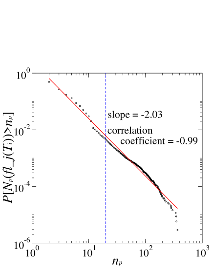
Figure 2: LLCD plots of $N_{p}\left(fl\_j\left(T_{i}\right)\right)$.

4 Hop count estimation

4.1 Estimation technique

To study hop counts between two nodes from the given trace data, we used the TTL (time to live) field of an IP packet. As its value is decreased when an IP packet passes a router, we can estimate hop counts between the source node and measuring point from the initial TTL value and the TTL value of the recieved packet. So, if we can obtain the hop counts from both the source and destination nodes to the measuring point, we can estimate the hop counts between these nodes . One difficulty with this approach is that the initial TTL values depend on the operating system or network equipment such as routers (see [3] for example). So first of all, we must determine the initial TTL value of source nodes. In this work, we used the approach of passive OS fingerprinting to estimate hop counts as exactly as possible. This technique is based on the principle that every system has its own IP stack implementation. That is, we can detect systems extremely accurately using some values recorded in IP packets they sent. More detailed information about passive OS fingerprinting can be found in [3]. In this work, we modified the source code of p.0.f.[5] and estimated the hop counts of each IP flow. In our study, we could estimate more than 10% of the systems for each trace. Here, we assume that we can regard statistics of these estimated flows as statistics of all flows.

4.2 Hop counts of greedy flows

For each flow $fl\_j\left(T_{i}\right)$ defined in Sec. 3, we estimated hop counts $hop\left(fl\_j\left(T_{i}\right)\right)$ using the above technique. Figure 3(a) shows the relationship between $hop\left(fl\_j\left(T_{i}\right)\right)$ and $N_{p}\left(fl\_j\left(T_{i}\right)\right)$ for a certain trace. Figure 3(b) shows the histogram of $hop\left(fl\_j\left(T_{i}\right)\right)$ for the same trace. The hop counts of greedy flows (above the dashed line in (a)) can be considered to be smaller than those of all flows.

Then we investigated the histogram of $hop\left(fl\_j\left(T_{i}\right)\right)$ for all traces. Figure 4 shows histograms of (a) all flows and (b) greedy flows. The average hop counts for greedy flows were smaller than those of all flows, and most greedy flows had relatively smaller hop counts. Actually, average hop counts were 19.85 for all flows and 17.92 for greedy flows (see dashed lines in Figure 4). These results can be interpreted using the fact that the RTTs of flows with smaller hop counts tend to be smaller as demonstrated in [1], and TCP flows with smaller RTTs can make their window sizes larger following the mechanism of TCP flow control. That is, TCP flows with smaller hop counts can make their window sizes larger, and be greedier.

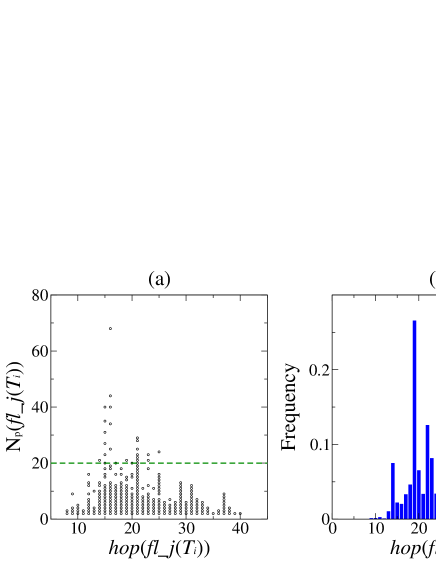
Figure 3: (a) $hop\left(fl\_j\left(T_{i}\right)\right)$ versus $N_{p}\left(fl\_j\left(T_{i}\right)\right)$, (b) histogram of $hop\left(fl\_j\left(T_{i}\right)\right)$.

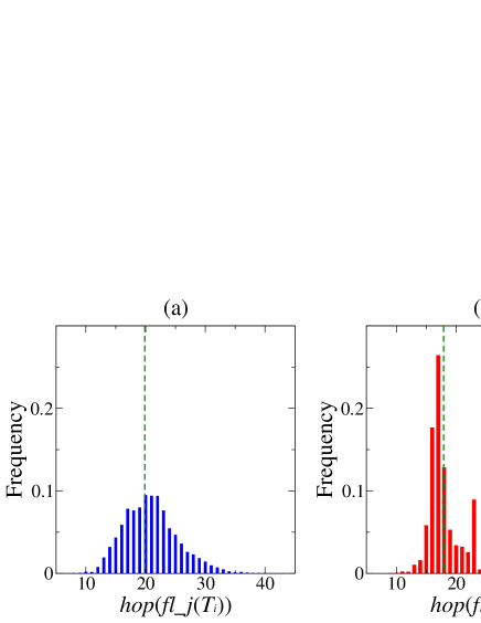
Figure 4: Histogram of $hop\left(fl\_j\left(T_{i}\right)\right)$ for (a) all flows, (b) greedy flows.

5 Breakdown of applications

We investigated the breakdown of applications for each flow using the port numbers (Table 1). We can immediately see that the proportion of HTTP was much larger among greedy flows than all flows. So it might be reasonable to assume that HTTP plays an important role in making greedy flows. We will focus on causal mechanisms of why HTTP flows are greedier than other applications, and the relationship with hop counts in our next work.

Table 1: Breakdown of applications

	All flows	Greedy flows
HTTP	54%	70%
other TCP	38%	20%
UDP	7%	6%
other	1%	4%

6 Summary

To study mechanisms that cause the non-Gaussian nature of network traffic, we investigated the properties of greedy IP flows. Our main findings are as follows. (1) Hop counts of greedy flows were relatively smaller than those of all flows. (2) HTTP was the main application for greedy flows. Since the most popular application on the Internet today is server-client type file-transfer applications such as WWW, we believe that the results of this work suggest the ubiquitous existence of greedy flows, which causes the non-Gaussian nature of network traffic.

References

- [1] Keita Fujii, Shigeki Goto, Correlation between Hop Count and Packet Transfer Time, APAN/IWS2000, February 2000
- [2] Tatsuya Mori, Ryoichi Kawahara, A study on the marginal distribution of network traffic. IEICE Technical Report, IN 2001-107, pp. 1-7, 2001
- [3] Lance Spitzner, Know Your Enemy: Passive Fingerprinting, http://project.honeynet.org/papers/finger/
-
[4]
WIDE MAWI Working Group Traffic Archive
http://tracer.csl.sony.co.jp/mawi/ -
[5]
passive OS fingerprinting tool p.0.f.
http://www.stearns.org/p0f/