Smoothed Analysis of Algorithms:
Why the Simplex Algorithm Usually Takes Polynomial Time

Abstract

We introduce the smoothed analysis of algorithms, which continuously interpolates between the worst-case and average-case analyses of algorithms. In smoothed analysis, we measure the maximum over inputs of the expected performance of an algorithm under small random perturbations of that input. We measure this performance in terms of both the input size and the magnitude of the perturbations. We show that the simplex algorithm has smoothed complexity polynomial in the input size and the standard deviation of Gaussian perturbations.

List of Theorems, Lemmas, Corollaries and Propositions

1. Theorem 2.5.2 (Blaschke).
2. Theorem 4.0.1 (Shadow Size).
3. Theorem 5.0.1 (Main).

1. Lemma 2.3.3 (Comparing expectations).
2. Lemma 2.3.4 (Similar distributions).
3. Lemma 2.3.5 (Combination lemma).
4. Lemma 2.3.6 (Generalized combination lemma).
5. Lemma 2.3.7 (Almost polynomial densities).
6. Lemma 2.4.2 (Smoothness of Gaussians).
7. Lemma 2.4.11 (Comparing Gaussian tails).
8. Lemma 3.3.5 (Shadow path of $LP^{+}$).
9. Lemma 4.0.6 (Discretization in limit).
10. Lemma 4.0.7 (Angle bound).
11. Lemma 4.0.11 (Angle bound given optSimp).
12. Lemma 4.0.12 (Division into distance and angle).
13. Lemma 4.1.1 (Distance bound).
14. Lemma 4.1.2 (Distance bound in plane).
15. Lemma 4.1.3 (Height of simplex).
16. Lemma 4.2.1 (Angle of incidence).
17. Lemma 4.2.2 (Angle of incidence, II).
18. Lemma 4.2.3 (Points under plane).
19. Lemma 5.1.1 (Many good choices).
20. Lemma 5.1.6 (Probability of $Y_{K}^{j}$).
21. Lemma 5.1.7 (Sum over $j$ of $Y_{K}^{j}$).
22. Lemma 5.1.8 (Sum over $K$ and $j$ of $Y_{K}^{j}$).
23. Lemma 5.1.9 (Relating $X$s to $Y$s).
24. Lemma 5.1.10 (Geometric condition for bad $I$).
25. Lemma 5.1.11 (Big height, small coefficient).
26. Lemma 5.1.12 (Probability of bad geometry).
27. Lemma 5.2.1 (LP’).
28. Lemma 5.2.2 (probability of small $\mbox{\bf s}_{\textbf{min}}\left(\boldsymbol{\tilde{\mathit{A}}}_{\mathcal{I}(\boldsymbol{\mathit{A}})}\right)$).
29. Lemma 5.2.3 (From $\tilde{\boldsymbol{\mathit{a}}}$).
30. Lemma 5.2.4 (Changing $\boldsymbol{\alpha}$ to $\boldsymbol{\tilde{\alpha}}$).
31. Lemma 5.2.5 (Approximation of $\boldsymbol{\alpha}$ by $\boldsymbol{\tilde{\alpha}}$).
32. Lemma 5.2.7 (Proper subset).
33. Lemma 5.2.9 (Jacobian of $\Psi$).
34. Lemma 5.2.10 (Bound on Jacobian of $\Psi$).
35. Lemma 5.2.11 (Jacobian of $\Gamma_{\boldsymbol{\mathit{u}},\boldsymbol{\mathit{v}}}$).
36. Lemma 5.2.12 (Jacobian of $\Gamma_{\boldsymbol{\mathit{u}},\boldsymbol{\mathit{v}}}$ in 2D).
37. Lemma 5.3.1 (LP+).
38. Lemma 5.3.2 ($LP^{+}$ Shadow, part 2).
39. Lemma 5.3.3 ($\hat{\nu}$).
40. Lemma 5.3.4 (Almost Gaussian).
41. Lemma 5.3.5 (Almost Gaussian, single variable).
42. Lemma 5.3.6 (Almost Gaussian, pointwise).
43. Lemma 5.3.7 (Almost Gaussian, Jacobians).

1. Corollary 2.4.6 (A chi-square bound).
2. Corollary 2.5.3 (Blaschke with $s$).
3. Corollary 4.3.1 ($\left\|\boldsymbol{\mathit{a}}_{i}\right\|$ free).
4. Corollary 4.3.2 (Gaussians free).
5. Corollary 4.3.3 ($y_{i}$ free).
6. Corollary 5.1.2 (probability of small $\mbox{\bf s}_{\textbf{min}}\left(\boldsymbol{\mathit{A}}_{\mathcal{I}(\boldsymbol{\mathit{A}})}\right)$).
7. Corollary 5.1.3 (probability of $\kappa$ in $\mathcal{K}$).

1. Proposition 2.2.2 (Vectors norms).
2. Proposition 2.2.4 (Properties of matrix norm).
3. Proposition 2.2.6 (Properties of $\mbox{\bf s}_{\textbf{min}}\left(\right)$).
4. Proposition 2.3.1 (Average $\leq$ maximum).
5. Proposition 2.3.2 (Expectation on sub-domain).
6. Proposition 2.4.1 (Additivity of Gaussians).
7. Proposition 2.4.3 (Restrictions of Gaussians).
8. Proposition 2.4.4 (Gaussian measure of halfspaces).
9. Proposition 2.4.5 (Chi-Square bound).
10. Proposition 2.4.7 (Gaussian near point or plane).
11. Proposition 2.4.8 (Gamma Inequality).
12. Proposition 2.4.9 (Non-central Gaussian near the origin).
13. Proposition 2.4.10 (Gaussian tail bound).
14. Proposition 2.4.12 (Monotonicity of Gaussian density).
15. Proposition 2.5.1 (Change of variables).
16. Proposition 2.5.4 (Latitude and longitude).
17. Proposition 3.2.2 (Duality).
18. Proposition 3.2.3 (Detecting unbounded programs).
19. Proposition 3.3.1 (Initial simplex of $LP^{\prime}$).
20. Proposition 3.3.2 (relation of $M$ and $\kappa$).
21. Proposition 3.3.3 (Unbounded programs).
22. Proposition 3.3.4 (Bounded programs).
23. Proposition 4.0.5 (Measure of P).
24. Proposition 4.0.9 ($P\subset P^{j}_{I}$).
25. Proposition 5.0.2 (trivial shadow bounds).
26. Proposition 5.1.4 (size of $\mathcal{K}$).
27. Proposition 5.2.6 (Volume dilation).

1 Introduction

The Analysis of Algorithms community has been challenged by the existence of remarkable algorithms that are known by scientists and engineers to work well in practice, but whose theoretical analyses are negative or inconclusive. The root of this problem is that algorithms are usually analyzed in one of two ways: by worst-case or average-case analysis. Worst-case analysis can improperly suggest that an algorithm will perform poorly by examining its performance under the most contrived circumstances. Average-case analysis was introduced to provide a less pessimistic measure of the performance of algorithms, and many practical algorithms perform well on the random inputs considered in average-case analysis. However, average-case analysis may be unconvincing as the inputs encountered in many application domains may bear little resemblance to the random inputs that dominate the analysis.

We propose an analysis that we call smoothed analysis which can help explain the success of algorithms that have poor worst-case complexity and whose inputs look sufficiently different from random that average-case analysis cannot be convincingly applied. In smoothed analysis, we measure the performance of an algorithm under slight random perturbations of arbitrary inputs. In particular, we consider Gaussian perturbations of inputs to algorithms that take real inputs, and we measure the running times of algorithms in terms of their input size and the standard deviation of the Gaussian perturbations.

We show that the simplex method has polynomial smoothed complexity. The simplex method is the classic example of an algorithm that is known to perform well in practice but which takes exponential time in the worst case [KM72, Mur80, GS79, Gol83, AC78, Jer73, AZ99]. In the late 1970’s and early 1980’s the simplex method was shown to converge in expected polynomial time on various distributions of random inputs by researchers including Borgwardt, Smale, Haimovich, Adler, Karp, Shamir, Megiddo, and Todd [Bor80, Bor77, Sma83, Hai83, AKS87, AM85, Tod86]. These works introduced novel probabilistic tools to the analysis of algorithms, and provided some intuition as to why the simplex method runs so quickly. However, these analyses are dominated by “random looking” inputs: even if one were to prove very strong bounds on the higher moments of the distributions of running times on random inputs, one could not prove that an algorithm performs well in any particular small neighborhood of inputs.

To bound expected running times on small neighborhoods of inputs, we consider linear programming problems in the form

maximize $$\boldsymbol{\mathit{z}}^{T}\boldsymbol{\mathit{x}}$$ (1)

subject to $$\boldsymbol{\mathit{A}}\boldsymbol{\mathit{x}}\leq\boldsymbol{\mathit{y}},$$

and prove that for every vector $\boldsymbol{\mathit{z}}$ and every matrix $\bar{\boldsymbol{\mathit{A}}}$ and vector $\bar{\boldsymbol{\mathit{y}}}$, the expectation over standard deviation $\sigma\left(\max_{i}\left\|(\bar{y}_{i},\bar{\boldsymbol{\mathit{a}}}_{i})\right\|\right)$ Gaussian perturbations $\boldsymbol{\mathit{A}}$ and $\boldsymbol{\mathit{y}}$ of $\bar{\boldsymbol{\mathit{A}}}$ and $\bar{\boldsymbol{\mathit{y}}}$ of the time taken by a two-phase shadow-vertex simplex method to solve such a linear program is polynomial in $1/\sigma$ and the dimensions of $\boldsymbol{\mathit{A}}$.

1.1 Linear Programming and the Simplex Method

It is difficult to overstate the importance of linear programming to optimization. Linear programming problems arise in innumerable industrial contexts. Moreover, linear programming is often used as a fundamental step in other optimization algorithms. In a linear programming problem, one is asked to maximize or minimize a linear function over a polyhedral region.

Perhaps one reason we see so many linear programs is that we can solve them efficiently. In 1947, Dantzig [Dan51] introduced the simplex method, which was the first practical approach to solving linear programs and which remains widely used today. To state it roughly, the simplex method proceeds by walking from one vertex to another of the polyhedron defined by the inequalities in (1). At each step, it walks to a vertex that is better with respect to the objective function. The algorithm will either determine that the constraints are unsatisfiable, determine that the objective function is unbounded, or reach a vertex from which it cannot make progress, which necessarily optimizes the objective function.

Because of its great importance, other algorithms for linear programming have been invented. In 1979, Khachiyan [Kha79] applied the ellipsoid algorithm to linear programming and proved that it always converged in time polynomial in $d$, $n$, and $L$—the number of bits needed to represent the linear program. However, the ellipsoid algorithm has not been competitive with the simplex method in practice. In contrast, the interior-point method introduced in 1984 by Karmarkar [Kar84], which also runs in time polynomial in $d$, $n$, and $L$, has performed very well: variations of the interior point method are competitive with and occasionally superior to the simplex method in practice.

In spite of half a century of attempts to unseat it, the simplex method remains the most popular method for solving linear programs. However, there has been no satisfactory theoretical explanation of its excellent performance. A fascinating approach to understanding the performance of the simplex method has been the attempt to prove that there always exists a short walk from each vertex to the optimal vertex. The Hirsch conjecture states that there should always be a walk of length at most $n-d$. Significant progress on this conjecture was made by Kalai and Kleitman [KK92], who proved that there always exists a walk of length at most $n^{\log_{2}d+2}$. However, the existence of such a short walk does not imply that the simplex method will find it.

A simplex method is not completely defined until one specifies its pivot rule—the method by which it decides which vertex to walk to when it has many to choose from. There is no deterministic pivot rule under which the simplex method is known to take a sub-exponential number of steps. In fact, for almost every deterministic pivot rule there is a family of polytopes on which it is known to take an exponential number of steps [KM72, Mur80, GS79, Gol83, AC78, Jer73]. (See [AZ99] for a survey and a unified construction of these polytopes). The best present analysis of randomized pivot rules shows that they take expected time $n^{O(\sqrt{d})}$[Kal92, MSW96], which is quite far from the polynomial complexity observed in practice. This inconsistency between the exponential worst-case behavior of the simplex method and its everyday practicality leave us wanting a more reasonable theoretical analysis.

Various average-case analyses of the simplex method have been performed. Most relevant to this paper is the analysis of Borgwardt [Bor77, Bor80], who proved that the simplex method with the shadow vertex pivot rule runs in expected polynomial time for polytopes whose constraints are drawn independently from spherically symmetric distributions (e.g. Gaussian distributions centered at the origin). Independently, Smale [Sma83, Sma82] proved bounds on the expected running time of Lemke’s self-dual parametric simplex algorithm on linear programming problems chosen from a spherically-symmetric distribution. Smale’s analysis was substantially improved by Megiddo [Meg86].

While these average-case analyses are significant accomplishments, it is not clear whether they actually provide intuition for what happens on typical inputs. Edelman [Ede92] writes on this point:

What is a mistake is to psychologically link a random matrix with the intuitive notion of a “typical” matrix or the vague concept of “any old matrix.”

Another model of random linear programs was studied in a line of research initiated independently by Haimovich [Hai83] and Adler [Adl83]. Their works considered the maximum over matrices, $\boldsymbol{\mathit{A}}$, of the expected time taken by parametric simplex methods to solve linear programs over these matrices in which the directions of the inequalities are chosen at random. As this framework considers the maximum of an average, it may be viewed as a precursor to smoothed analysis—the distinction being that the random choice of inequalities cannot be viewed as a perturbation, as different choices yield radically different linear programs. Haimovich and Adler both proved that parametric simplex methods would take an expected linear number of steps to go from the vertex minimizing the objective function to the vertex maximizing the objective function, even conditioned on the program being feasible. While their theorems confirmed the intuitions of many practitioners, they were geometric rather than algorithmic as it was not clear how an algorithm would locate either vertex. Building on these analyses, Todd [Tod86], Adler and Megiddo [AM85], and Adler, Karp and Shamir [AKS87] analyzed parametric algorithms for linear programming under this model and proved quadratic bounds on their expected running time. While the random inputs considered in these analyses are not as special as the random inputs obtained from spherically symmetric distributions, the model of randomly flipped inequalities provokes some similar objections.

1.2 Smoothed Analysis of Algorithms and Related Work

We introduce the smoothed analysis of algorithms in the hope that it will help explain the good practical performance of many algorithms that worst-case does not and for which average-case analysis is unconvincing. Our first application of the smoothed analysis of algorithms will be to the simplex method. We will consider the maximum over $\bar{\boldsymbol{\mathit{A}}}$ and $\bar{\boldsymbol{\mathit{y}}}$ of the expected running time of the simplex method on inputs of the form

maximize $$\boldsymbol{\mathit{z}}^{T}\boldsymbol{\mathit{x}}$$ (2)

subject to $$(\bar{\boldsymbol{\mathit{A}}}+\boldsymbol{\mathit{G}})\boldsymbol{\mathit{x}}\leq(\bar{\boldsymbol{\mathit{y}}}+\boldsymbol{\mathit{h}}),$$

where we let $\bar{\boldsymbol{\mathit{A}}}$ and $\bar{\boldsymbol{\mathit{y}}}$ be arbitrary and $\boldsymbol{\mathit{G}}$ and $\boldsymbol{\mathit{h}}$ be a matrix and a vector of independently chosen Gaussian random variables of mean $0$ and standard deviation $\sigma\left(\max_{i}\left\|(\bar{y}_{i},\bar{\boldsymbol{\mathit{a}}}_{i})\right\|\right)$. If we let $\sigma$ go to $0$, then we obtain the worst-case complexity of the simplex method; whereas, if we let $\sigma$ be so large that $\boldsymbol{\mathit{G}}$ swamps out $\boldsymbol{\mathit{A}}$, we obtain the average-case analyzed by Borgwardt. By choosing polynomially small $\sigma$, this analysis combines advantages of worst-case and average-case analysis, and roughly corresponds to the notion of imprecision in low-order digits.

In a smoothed analysis of an algorithm, we assume that the inputs to the algorithm are subject to slight random perturbations, and we measure the complexity of the algorithm in terms of the input size and the standard deviation of the perturbations. If an algorithm has low smoothed complexity, then one should expect it to work well in practice since most real-world problems are generated from data that is inherently noisy. Another way of thinking about smoothed complexity is to observe that if an algorithm has low smoothed complexity, then one must be unlucky to choose an input instance on which it performs poorly.

We now provide some definitions for the smoothed analysis of algorithms that take real or complex inputs. For an algorithm $A$ and input $\boldsymbol{\mathit{x}}$, let

$$\mathcal{C}_{A}(\boldsymbol{\mathit{x}})$$

be a complexity measure of $A$ on input $\boldsymbol{\mathit{x}}$. Let $X$ be the domain of inputs to $A$, and let $X_{n}$ be the set of inputs of size $n$. The size of an input can be measured in various ways. Standard measures are the number of real variables contained in the input and the sums of the bit-lengths of the variables. Using this notation, one can say that $A$ has worst-case $\mathcal{C}$-complexity $f(n)$ if

$$\max_{\boldsymbol{\mathit{x}}\in X_{n}}(\mathcal{C}_{A}(\boldsymbol{\mathit{x}}))=f(n).$$

Given a family of distributions $\mu_{n}$ on $X_{n}$, we say that $A$ has average-case $\mathcal{C}$-complexity $f(n)$ under $\mu$ if

$$\operatorname{\textbf{E}}\displaylimits_{\boldsymbol{\mathit{x}}\stackrel{{\scriptstyle\,\mu_{n}}}{{\leftarrow}}X_{n}}\left[\mathcal{C}_{A}(\boldsymbol{\mathit{x}})\right]=f(n).$$

Similarly, we say that $A$ has smoothed $\mathcal{C}$-complexity $f(n,\sigma)$ if

$$\max_{\boldsymbol{\mathit{x}}\in X_{n}}\operatorname{\textbf{E}}\displaylimits_{\boldsymbol{\mathit{g}}}\left[\mathcal{C}_{A}(\boldsymbol{\mathit{x}}+\left(\sigma\left\|\boldsymbol{\mathit{x}}\right\|_{?}\right)\boldsymbol{\mathit{g}})\right]=f(n,\sigma),$$ (3)

where $\left(\sigma\left\|\boldsymbol{\mathit{x}}\right\|_{?}\right)\boldsymbol{\mathit{g}}$ is a vector of Gaussian random variables of mean $0$ and standard deviation $\sigma\left\|\boldsymbol{\mathit{x}}\right\|_{?}$ and $\left\|\boldsymbol{\mathit{x}}\right\|_{?}$ is a measure of the magnitude of $\boldsymbol{\mathit{x}}$, such as the largest element or the norm. We say that an algorithm has polynomial smoothed complexity if its smoothed complexity is polynomial in $n$ and $1/\sigma$. In Section 6, we present some generalizations of the definition of smoothed complexity that might prove useful. To further contrast smoothed analysis with average-case analysis, we note that the probability mass in (3) is concentrated in a region of radius $O(\sigma\sqrt{n})$ and volume at most $O(\sigma\sqrt{n})^{n}$, and so, when $\sigma$ is small, this region contains an exponentially small fraction of the probability mass in an average-case analysis. Thus, even an extension of average-case analysis to higher moments will not imply meaningful bounds on smoothed complexity.

A discrete analog of smoothed analysis has been studied in a collection of works inspired by Santha and Vazirani’s semi-random source model [SV86]. In this model, an adversary generates an input, and each bit of this input has some probability of being flipped. Blum and Spencer [BS95] design a polynomial-time algorithm that $k$-colors $k$-colorable graphs generated by this model. Feige and Krauthgamer [FK] analyze a model in which the adversary is more powerful, and use it to show that Turner’s algorithm [Tur86] for approximating the bandwidth performs well on semi-random inputs. They also improve Turner’s analysis. Feige and Kilian [FK98] present polynomial-time algorithms that recover large independent sets, $k$-colorings, and optimal bisections in semi-random graphs. They also demonstrate that significantly better results would lead to surprising collapses of complexity classes.

1.3 Our Results

We consider the maximum over $\boldsymbol{\mathit{z}}$, $\bar{\boldsymbol{\mathit{y}}}$, and $\bar{\boldsymbol{\mathit{a}}}_{1},\ldots,\bar{\boldsymbol{\mathit{a}}}_{n}$ of the expected time taken by a two-phase shadow vertex simplex method to solve linear programming problems of the form

maximize $$\boldsymbol{\mathit{z}}^{T}\boldsymbol{\mathit{x}}$$ (4)

subject to $$\left<\boldsymbol{\mathit{a}}_{i}|\boldsymbol{\mathit{x}}\right>\leq y_{i},\mbox{ for $1\leq i\leq n$,}$$

where each $\boldsymbol{\mathit{a}}_{i}$ is a Gaussian random vector of standard deviation $\sigma\max_{i}\left\|(\bar{y}_{i},\bar{\boldsymbol{\mathit{a}}}_{i})\right\|$ centered at $\bar{\boldsymbol{\mathit{a}}}_{i}$, and each $y_{i}$ is a Gaussian random variable of standard deviation $\sigma\max_{i}\left\|(\bar{y}_{i},\bar{\boldsymbol{\mathit{a}}}_{i})\right\|$ centered at $\bar{y}_{i}$.

We begin by considering the case in which $\boldsymbol{\mathit{y}}=\mathbf{1}$, $\left\|\bar{\boldsymbol{\mathit{a}}}_{i}\right\|\leq 1$, and $\sigma<1/3\sqrt{d\ln n}$. In this case, our first result, Theorem 4.0.1, says that for every vector $\boldsymbol{\mathit{t}}$ the expected size of the shadow of the polytope—the projection of the polytope defined by the equations (4) onto the plane spanned by $\boldsymbol{\mathit{t}}$ and $\boldsymbol{\mathit{z}}$—is polynomial in $n$, the dimension, and $1/\sigma$. This result is the geometric foundation of our work, but it does not directly bound the running time of an algorithm, as the shadow relevant to the analysis of an algorithm depends on the perturbed program and cannot be specified beforehand as the vector $\boldsymbol{\mathit{t}}$ must be. In Section 3.3, we describe a two-phase shadow-vertex simplex algorithm, and in Section 5 we use Theorem 4.0.1 as a black box to show that it takes expected time polynomial in $n$, $d$, and $1/\sigma$ in the case described above.

Efforts have been made to analyze how much the solution of a linear program can change as its data is perturbed. For an introduction to such analyses, and an analysis of the complexity of interior point methods in terms of the resulting condition number, we refer the reader to the work of Renegar [Ren95b, Ren95a, Ren94].

1.4 Intuition Through Condition Numbers

For those already familiar with the simplex method and condition numbers, we include this section to provide some intuition for why our results should be true.

Our analysis will exploit geometric properties of the condition number of a matrix, rather than of a linear program. We start with the observation that if a corner of a polytope is specified by the equation $A_{I}\boldsymbol{\mathit{x}}=\boldsymbol{\mathit{y}}_{I}$, where $I$ is a $d$-set, then the condition number of the matrix $A_{I}$ provides a good measure of how far the corner is from being flat. Moreover, it is relatively easy to show that if $A$ is subject to perturbation, then it is unlikely that $A_{I}$ has poor condition number. So, it seems intuitive that if $A$ is perturbed, then most corners of the polytope should have angles bounded away from being flat. This already provides some intuition as to why the simplex method should run quickly: one should make reasonable progress as one rounds a corner if it is not too flat.

There are two difficulties in making the above intuition rigorous: the first is that even if $A_{I}$ is well-conditioned for most sets $I$, it is not clear that $A_{I}$ will be well-conditioned for most sets $I$ that are bases of corners of the polytope. The second difficulty is that even if most corners of the polytope have reasonable condition number, it is not clear that a simplex method will actually encounter many of these corners. By analyzing the shadow vertex pivot rule, it is possible to resolve both of these difficulties.

The first advantage of studying the shadow vertex pivot rule is that its analysis comes down to studying the expected sizes of shadows of the polytope. From the specification of the plane onto which the polytope will be projected, one obtains a characterization of all the corners that will be in the shadow, thereby avoiding the complication of an iterative characterization. The second advantage is that these corners are specified by the property that they optimize a particular objective function, and using this property one can actually bound the probability that they are ill-conditioned. While the results of Section 4 are not stated in these terms, this is the intuition behind them.

Condition numbers also play a fundamental role in our analysis of the shadow-vertex algorithm. The analysis of the algorithm differs from the mere analysis of the sizes of shadows in that, in the study of an algorithm, the plane onto which the polytope is projected depends upon the polytope itself. This correlation of the plane with the polytope complicates the analysis, but is also resolved through the help of condition numbers. In our analysis, we view the perturbation as the composition of two perturbations, where the second is small relative to the first. We show that our choice of the plane onto which we project the shadow is well-conditioned with high probability after the first perturbation. That is, we show that the second perturbation is unlikely to substantially change the plane onto which we project, and therefore unlikely to substantially change the shadow. Thus, it suffices to measure the expected size of the shadow obtained after the second perturbation onto the plane that would have been chosen after just the first perturbation.

The technical lemma that enables this analysis, Lemma 5.1.1, is a concentration result that proves that it is highly unlikely that almost all of the minors of a random matrix have poor condition number. This analysis also enables us to show that it is highly unlikely that we will need a large “big-$M$” in phase I of our algorithm.

We note that the condition numbers of the $A_{I}$s have been studied before in the complexity of linear programming algorithms. The condition number $\bar{\chi}_{A}$ of Vavasis and Ye [VY96] measures the condition number of the worst sub-matrix $A_{I}$, and their algorithm runs in time proportional to $\ln(\bar{\chi}_{A})$. Todd, Tunçel, and Ye [TTY01] have shown that for a Gaussian random matrix the expectation of $\ln(\bar{\chi}_{A})$ is $O(\min(d\ln n,n))$. That is, they show that it is unlikely that any $A_{I}$ is exponentially ill-conditioned. It is relatively simple to apply the techniques of Section 5.1 to obtain a similar result in the smoothed case. We wonder whether our concentration result that it is exponentially unlikely that many $A_{I}$ are even polynomially ill-conditioned could be used to obtain a better smoothed analysis of the Vavasis-Ye algorithm.

1.5 Discussion

One can debate whether the definition of polynomial smoothed complexity should be that an algorithm have complexity polynomial in $1/\sigma$ or $\log(1/\sigma)$. We believe that the choice of being polynomial in $1/\sigma$ will prove more useful as the other definition is too strong and quite similar to the notion of being polynomial in the worst case. In particular, one can convert any algorithm for linear programming whose smoothed complexity is polynomial in $d$, $n$ and $\log(1/\sigma)$ into an algorithm whose worst-case complexity is polynomial in $d$, $n$, and $L$. That said, one should certainly prefer complexity bounds that are lower as a function of $1/\sigma$, $d$ and $n$.

We also remark that a simple examination of the constructions that provide exponential lower bounds for various pivot rules [KM72, Mur80, GS79, Gol83, AC78, Jer73] reveals that none of these pivot rules have smoothed complexity polynomial in $n$ and sub-polynomial in $1/\sigma$. That is, these constructions are unaffected by exponentially small perturbations.

2 Notation and Mathematical Preliminaries

In this section, we define the notation that will be used in the paper. We will also review some background from mathematics and derive a few simple statements that we will need. The reader should probably skim this section now, and save a more detailed examination for when the relevant material is referenced.

• $[n]$ denotes the set of integers between 1 and $n$, and $\binom{[n]}{k}$ denotes the subsets of $[n]$ of size $k$.

• Subsets of $[n]$ are denoted by the capital Roman letters $I,J,L,K$. $\mathcal{M}$ will denote a subset of integers, and $\mathcal{K}$ will denote a set of subsets of $[n]$.

• Subsets of ${\rm I\kern-2.0ptR}^{?}$ are denoted by the capital Roman letters $A,B,P,Q,R,S,T,U,V$.

• Vectors in ${\rm I\kern-2.0ptR}^{?}$ are denoted by bold lower-case Roman letters, such as $\boldsymbol{\mathit{a}}_{i},\bar{\boldsymbol{\mathit{a}}}_{i},\tilde{\boldsymbol{\mathit{a}}}_{i}$, $\boldsymbol{\mathit{b}}_{i},\boldsymbol{\mathit{c}}_{i}$, $\boldsymbol{d}_{i},\boldsymbol{\mathit{h}}$, $\boldsymbol{\mathit{t}},\boldsymbol{\mathit{q}},\boldsymbol{\mathit{z}},\boldsymbol{\mathit{y}}$.

• Whenever a vector, say $\boldsymbol{\mathit{a}}\in{\rm I\kern-2.0ptR}^{d}$ is present, its components will be denoted by lower-case Roman letters with subscripts, such as $a_{1},\ldots,a_{d}$.

• Whenever a collection of vectors, such as $\boldsymbol{\mathit{a}}_{1},\ldots,\boldsymbol{\mathit{a}}_{n}$, are present, the similar bold upper-case letter, such as $\boldsymbol{\mathit{A}}$, will denote the matrix of these vectors. For $I\in\binom{[n]}{k}$, $\boldsymbol{\mathit{A}}_{I}$ will denote the matrix of those $\boldsymbol{\mathit{a}}_{i}$ for which $i\in I$.

• Matrices are denoted by bold upper-case Roman letters, such as $\boldsymbol{\mathit{A}},\bar{\boldsymbol{\mathit{A}}},\boldsymbol{\tilde{\mathit{A}}},\boldsymbol{\mathit{B}},\boldsymbol{\mathit{M}}$ and $\boldsymbol{\mathit{R}}_{\boldsymbol{\omega}}$.

• $S^{d-1}$ denotes the unit sphere in ${\rm I\kern-2.0ptR}^{d}$.

• Vectors in $S^{?}$ will be denoted by bold Greek letters, such as $\boldsymbol{\omega},\boldsymbol{\psi},\boldsymbol{\tau}$.

• Generally speaking, univariate quantities with scale, such as lengths or heights, will be represented by lower case Roman letters such as $c$, $h$, $l$, $r$, $s$, and $t$. The principal exceptions are that $\kappa$ and $M$ will also denote such quantities.

• Quantities without scale, such as the ratios of quantities with scale or affine coordinates, will be represented by lower case Greek letters such as $\alpha,\beta,\lambda,\xi,\zeta$. $\boldsymbol{\alpha}$ will denote a vector of such quantities such as $(\alpha_{1},\ldots,\alpha_{d})$.

• Density functions are denoted by lower case Greek letters such as $\mu$ and $\nu$.

• The standard deviations of Gaussian random variables are denoted by lower-case Greek letters such as $\sigma,\tau$ and $\rho$.

• Indicator random variables are denoted by upper case Roman letters, such as $A$, $B$, $E$, $F$, $V$, $W$, $X$, $Y$, and $Z$

• Functions into the reals or integers will be denoted by calligraphic upper-case letters, such as $\mathcal{F},\mathcal{G},\mathcal{S}^{+},\mathcal{S}^{\prime},\mathcal{T}$.

• Functions into ${\rm I\kern-2.0ptR}^{?}$ are denoted by upper-case Greek letters, such as $\Phi_{\epsilon},\Upsilon,\Psi$.

• $\left<\boldsymbol{\mathit{x}}|\boldsymbol{\mathit{y}}\right>$ denotes the inner product of vectors $\boldsymbol{\mathit{x}}$ and $\boldsymbol{\mathit{y}}$.

• For vectors $\boldsymbol{\omega}$ and $\boldsymbol{\mathit{z}}$, we let $\mbox{{\bf angle}}\left(\boldsymbol{\omega},\boldsymbol{\mathit{z}}\right)$ denote the angle between these vectors at the origin.

• The logarithm base 2 is written $\lg$ and the natural logarithm is written $\ln$.

• The probability of an event $A$ is written $\operatorname{\textbf{Pr}}\displaylimits\left[A\right]$, and the expectation of a variable $X$ is written $\operatorname{\textbf{E}}\displaylimits\left[X\right]$.

• The indicator random variable for an event $A$ is written $\left[A\right]$.

2.1 Geometric Definitions

For the following definitions, we let $\boldsymbol{\mathit{a}}_{1},\ldots,\boldsymbol{\mathit{a}}_{k}$ denote a set of vectors in ${\rm I\kern-2.0ptR}^{d}$.

• $\textbf{Span}\left(\boldsymbol{\mathit{a}}_{1},\ldots,\boldsymbol{\mathit{a}}_{k}\right)$ denotes the subspace spanned by $\boldsymbol{\mathit{a}}_{1},\ldots,\boldsymbol{\mathit{a}}_{k}$.

• $\mbox{{\bf Aff}}\left(\boldsymbol{\mathit{a}}_{1},\ldots,\boldsymbol{\mathit{a}}_{k}\right)$ denotes the hyperplane that is the affine span of $\boldsymbol{\mathit{a}}_{1},\ldots,\boldsymbol{\mathit{a}}_{k}$: the set of points $\sum_{i}\alpha_{i}\boldsymbol{\mathit{a}}_{i}$, where $\sum_{i}\alpha_{i}=1$, for all $i$.

• $\mbox{{ConvHull}}\left(\boldsymbol{\mathit{a}}_{1},\ldots,\boldsymbol{\mathit{a}}_{k}\right)$ denotes the convex hull of $\boldsymbol{\mathit{a}}_{1},\ldots,\boldsymbol{\mathit{a}}_{k}$.

• $\mbox{{\bf Cone}}\left(\boldsymbol{\mathit{a}}_{1},\ldots,\boldsymbol{\mathit{a}}_{k}\right)$ denotes the positive cone through $\boldsymbol{\mathit{a}}_{1},\ldots,\boldsymbol{\mathit{a}}_{k}$: the set of points $\sum_{i}\alpha_{i}\boldsymbol{\mathit{a}}_{i}$, for $\alpha_{i}\geq 0$.

• $\bigtriangleup\left(\boldsymbol{\mathit{a}}_{1},\ldots,\boldsymbol{\mathit{a}}_{d}\right)$ denotes the simplex $\mbox{{ConvHull}}\left(\boldsymbol{\mathit{a}}_{1},\ldots,\boldsymbol{\mathit{a}}_{d}\right)$.

For a linear program specified by $\boldsymbol{\mathit{a}}_{1},\ldots,\boldsymbol{\mathit{a}}_{n}$, $\boldsymbol{\mathit{y}}$ and $\boldsymbol{\mathit{z}}$, we will say that the linear program is in general position if

• The points $\boldsymbol{\mathit{a}}_{1},\ldots,\boldsymbol{\mathit{a}}_{n}$ are in general position with respect to $\boldsymbol{\mathit{y}}$, which means that for all $I\subset\binom{[n]}{d}$ and $\boldsymbol{\mathit{x}}=\boldsymbol{\mathit{A}}_{I}^{-1}\boldsymbol{\mathit{y}}_{I}$, and all $j\not\in I$, $\left<\boldsymbol{\mathit{a}}_{j}|\boldsymbol{\mathit{x}}\right>\not=y_{j}$.

• For all $I\subset\binom{[n]}{d-1}$, $\boldsymbol{\mathit{z}}\not\in\mbox{{\bf Cone}}\left(\boldsymbol{\mathit{A}}_{I}\right)$.

Furthermore, we will say that the linear program is in general position with respect to a vector $\boldsymbol{\mathit{t}}$ if the set of $\lambda$ for which there exists an $I\in\binom{[n]}{d-1}$ such that

$$(1-\lambda)\boldsymbol{\mathit{t}}+\lambda\boldsymbol{\mathit{z}}\in\mbox{{\bf Cone}}\left(\boldsymbol{\mathit{A}}_{I}\right)$$

is finite and does not contain $0$.

2.2 Vector and Matrix Norms

The material of this section is principally used in Sections 3.3 and 5.1. The following definitions and propositions are standard, and may be found in standard texts on Numerical Linear Algebra.

Definition 2.2.1 (Vector Norms).

For a vector $\boldsymbol{\mathit{x}}$, we define

• $\left\|\boldsymbol{\mathit{x}}\right\|=\sqrt{\sum_{i}x_{i}^{2}}$.

• $\left\|\boldsymbol{\mathit{x}}\right\|_{1}=\sum_{i}\left|x_{i}\right|$.

• $\left\|\boldsymbol{\mathit{x}}\right\|_{\infty}=\max_{i}\left|x_{i}\right|$.

Proposition 2.2.2 (Vectors norms).

For a vector $\boldsymbol{\mathit{x}}\in{\rm I\kern-2.0ptR}^{d}$,

$$\left\|\boldsymbol{\mathit{x}}\right\|\leq\left\|\boldsymbol{\mathit{x}}\right\|_{1}\leq\sqrt{d}\left\|\boldsymbol{\mathit{x}}\right\|.$$

Definition 2.2.3 (Matrix norm).

For a matrix $\boldsymbol{\mathit{A}}$, we define

$$\left\|\boldsymbol{\mathit{A}}\right\|\stackrel{{\scriptstyle\mathrm{def}}}{{=}}\max_{\boldsymbol{\mathit{x}}}\left\|\boldsymbol{\mathit{A}}\boldsymbol{\mathit{x}}\right\|/\left\|x\right\|.$$

Proposition 2.2.4 (Properties of matrix norm).

For $d$-by-$d$ matrices $\boldsymbol{\mathit{A}}$ and $\boldsymbol{\mathit{B}}$, and a $d$-vector $\boldsymbol{\mathit{x}}$,

1. $\left\|\boldsymbol{\mathit{A}}\boldsymbol{\mathit{x}}\right\|\leq\left\|\boldsymbol{\mathit{A}}\right\|\left\|\boldsymbol{\mathit{x}}\right\|$.

2. $\left\|\boldsymbol{\mathit{A}}\boldsymbol{\mathit{B}}\right\|\leq\left\|\boldsymbol{\mathit{A}}\right\|\left\|\boldsymbol{\mathit{B}}\right\|$.

3. $\left\|\boldsymbol{\mathit{A}}\right\|=\left\|\boldsymbol{\mathit{A}}^{T}\right\|$.

4. $\left\|\boldsymbol{\mathit{A}}\right\|\leq\sqrt{d}\max_{i}\left\|\boldsymbol{\mathit{a}}_{i}\right\|$, where $\boldsymbol{\mathit{A}}=(\boldsymbol{\mathit{a}}_{1},\ldots,\boldsymbol{\mathit{a}}_{d})$.

5. $\mbox{{\bf det}}\left(\boldsymbol{\mathit{A}}\right)\leq\left\|\boldsymbol{\mathit{A}}\right\|^{d}$.

Definition 2.2.5 ($\mbox{\bf s}_{\textbf{min}}\left(\right)$).

For a matrix $\boldsymbol{\mathit{A}}$, we define

$$\mbox{\bf s}_{\textbf{min}}\left(\boldsymbol{\mathit{A}}\right)\stackrel{{\scriptstyle\mathrm{def}}}{{=}}\left\|\boldsymbol{\mathit{A}}^{-1}\right\|^{-1}.$$

We recall that $\mbox{\bf s}_{\textbf{min}}\left(\boldsymbol{\mathit{A}}\right)$ is the smallest singular value of the matrix $\boldsymbol{\mathit{A}}$, and that it is not a norm.

Proposition 2.2.6 (Properties of $\mbox{\bf s}_{\textbf{min}}\left(\right)$).

For $d$-by-$d$ matrices $\boldsymbol{\mathit{A}}$ and $\boldsymbol{\mathit{B}}$,

1. $\mbox{\bf s}_{\textbf{min}}\left(\boldsymbol{\mathit{A}}\right)=\min_{\boldsymbol{\mathit{x}}}\left\|\boldsymbol{\mathit{A}}\boldsymbol{\mathit{x}}\right\|/\left\|\boldsymbol{\mathit{x}}\right\|$.

2. $\mbox{\bf s}_{\textbf{min}}\left(\boldsymbol{\mathit{B}}\right)\geq\mbox{\bf s}_{\textbf{min}}\left(\boldsymbol{\mathit{A}}\right)-\left\|\boldsymbol{\mathit{A}}-\boldsymbol{\mathit{B}}\right\|$ .

2.3 Probability

For an event, $A$, we let $\left[A\right]$ denote the indicator random variable for the event. We generally describe random variables by their density functions. If $\boldsymbol{\mathit{x}}$ has density $\mu$, then

$$\operatorname{\textbf{Pr}}\displaylimits\left[A(\boldsymbol{\mathit{x}})\right]\stackrel{{\scriptstyle\mathrm{def}}}{{=}}\int\left[A(\boldsymbol{\mathit{x}})\right]\mu(\boldsymbol{\mathit{x}})\,d\boldsymbol{\mathit{x}}\,.$$

If $B$ is another event, then

$$\operatorname{\textbf{Pr}}\displaylimits_{B}\left[A(\boldsymbol{\mathit{x}})\right]\stackrel{{\scriptstyle\mathrm{def}}}{{=}}\operatorname{\textbf{Pr}}\displaylimits\left[A(\boldsymbol{\mathit{x}})\big{|}B(\boldsymbol{\mathit{x}})\right]\stackrel{{\scriptstyle\mathrm{def}}}{{=}}\frac{\int\left[B(\boldsymbol{\mathit{x}})\right]\left[A(\boldsymbol{\mathit{x}})\right]\mu(\boldsymbol{\mathit{x}})\,d\boldsymbol{\mathit{x}}\,}{\int\left[B(\boldsymbol{\mathit{x}})\right]\mu(\boldsymbol{\mathit{x}})\,d\boldsymbol{\mathit{x}}\,}.$$

In a context where multiple densities are present, we will use use the notation $\operatorname{\textbf{Pr}}\displaylimits_{\mu}\left[A(\boldsymbol{\mathit{x}})\right]$ to indicate the probability of $A$ when $\boldsymbol{\mathit{x}}$ is distributed according to $\mu$.

In many situations, we will not know the density $\mu$ of a random variable $\boldsymbol{\mathit{x}}$, but rather a function $\nu$ such that $\nu(\boldsymbol{\mathit{x}})=c\mu(\boldsymbol{\mathit{x}})$ for some constant $c$. In this case, we will say that $\boldsymbol{\mathit{x}}$ has density proportional to $\nu$.

The following Propositions and Lemmas will play a prominent role in the proofs in this paper. The only one of these which might not be intuitively obvious is Lemma 2.3.5.

Proposition 2.3.1 (Average $\leq$ maximum).

Let $\mu(x,y)$ be a density function, and let $x$ and $y$ be distributed according to $\mu(x,y)$. If $A(x,y)$ is an event and $X(x,y)$ is random variable, then

$$\operatorname{\textbf{Pr}}\displaylimits_{x,y}\left[A(x,y)\right] \leq\max_{x}\operatorname{\textbf{Pr}}\displaylimits_{y}\left[A(x,y)\right],\text{ and}$$

$$\operatorname{\textbf{E}}\displaylimits_{x,y}\left[X(x,y)\right] \leq\max_{x}\operatorname{\textbf{E}}\displaylimits_{y}\left[X(x,y)\right],$$

where in the right-hand terms, $y$ is distributed according to the induced distribution $\mu(x,y)$.

Proposition 2.3.2 (Expectation on sub-domain).

Let $\boldsymbol{\mathit{x}}$ be a random variable and $A(\boldsymbol{\mathit{x}})$ an event. Let $P$ be a measurable subset of the domain of $\boldsymbol{\mathit{x}}$. Then,

$$\operatorname{\textbf{Pr}}\displaylimits_{\boldsymbol{\mathit{x}}\in P}\left[A(\boldsymbol{\mathit{x}})\right]\leq\operatorname{\textbf{Pr}}\displaylimits\left[A(\boldsymbol{\mathit{x}})\right]/\operatorname{\textbf{Pr}}\displaylimits\left[\boldsymbol{\mathit{x}}\in P\right].$$

Proof.

By the definition of conditional probability,

$$\operatorname{\textbf{Pr}}\displaylimits_{\boldsymbol{\mathit{x}}\in P}\left[A(\boldsymbol{\mathit{x}})\right] =\operatorname{\textbf{Pr}}\displaylimits\left[A(\boldsymbol{\mathit{x}})|\boldsymbol{\mathit{x}}\in P\right]$$

$$=\operatorname{\textbf{Pr}}\displaylimits\left[A(\boldsymbol{\mathit{x}})\text{ and }\boldsymbol{\mathit{x}}\in P\right]/\operatorname{\textbf{Pr}}\displaylimits\left[\boldsymbol{\mathit{x}}\in P\right],$$ by Bayes’ rule,

$$\leq\operatorname{\textbf{Pr}}\displaylimits\left[A(\boldsymbol{\mathit{x}})\right]/\operatorname{\textbf{Pr}}\displaylimits\left[\boldsymbol{\mathit{x}}\in P\right].$$

Lemma 2.3.3 (Comparing expectations).

Let $X$ and $Y$ be non-negative random variables and $A$ an event satisfying (1) $X\leq k$, (2) $\operatorname{\textbf{Pr}}\displaylimits\left[A\right]\geq 1-\epsilon$, and (3) there exists a constant $c$ such that $\operatorname{\textbf{E}}\displaylimits\left[X|A\right]\leq c\operatorname{\textbf{E}}\displaylimits\left[Y|A\right]$. Then,

$$\operatorname{\textbf{E}}\displaylimits\left[X\right]\leq c\operatorname{\textbf{E}}\displaylimits\left[Y\right]+\epsilon k.$$

Proof.

$$\operatorname{\textbf{E}}\displaylimits\left[X\right] =\operatorname{\textbf{E}}\displaylimits\left[X|A\right]\operatorname{\textbf{Pr}}\displaylimits\left[A\right]+\operatorname{\textbf{E}}\displaylimits\left[X|\mathbf{not}(A)\right]\operatorname{\textbf{Pr}}\displaylimits\left[\mathbf{not}(A)\right]$$

$$\leq c\operatorname{\textbf{E}}\displaylimits\left[Y|A\right]\operatorname{\textbf{Pr}}\displaylimits\left[A\right]+\epsilon k$$

$$\leq c\operatorname{\textbf{E}}\displaylimits\left[Y\right]+\epsilon k,$$

by Proposition 2.3.2.

Lemma 2.3.4 (Similar distributions).

Let $X$ be a non-negative random variable such that $X\leq k$. Let $\nu$ and $\mu$ be density functions for which there exists a set $S$ such that (1) $\operatorname{\textbf{Pr}}\displaylimits_{\nu}\left[S\right]>1-\epsilon$ and (2) there exists a constant $c\geq 1$ such that for all $a\in S$, $\nu(a)\leq c\mu(a)$. Then,

$$\operatorname{\textbf{E}}\displaylimits_{\nu}\left[X(a)\right]\leq c\operatorname{\textbf{E}}\displaylimits_{\mu}\left[X(a)\right]+k\epsilon.$$

Proof.

We write

$$\operatorname{\textbf{E}}\displaylimits_{\nu}\left[X\right] =\int_{a\in S}X(a)\nu(a)\,da\,+\int_{a\not\in S}X(a)\nu(a)\,da\,$$

$$\leq c\int_{a\in S}X(a)\mu(a)\,da\,+k\epsilon$$

$$\leq c\int_{a}X(a)\mu(a)\,da\,+k\epsilon$$

$$=c\operatorname{\textbf{E}}\displaylimits_{\mu}\left[X\right]+k\epsilon.$$

Lemma 2.3.5 (Combination lemma).

Let $x$ and $y$ be random variables distributed according to $\mu(x,y)$. Let $\mathcal{F}(x)$ and $\mathcal{G}(x,y)$ be non-negative functions and $\alpha$ and $\beta$ be constants such that

• $\forall\epsilon\geq 0$, $\operatorname{\textbf{Pr}}\displaylimits_{x,y}\left[\mathcal{F}(x)\leq\epsilon\right]\leq\alpha\epsilon$, and

• $\forall\epsilon\geq 0$, $\max_{x}\operatorname{\textbf{Pr}}\displaylimits_{y}\left[\mathcal{G}(x,y)\leq\epsilon\right]\leq(\beta\epsilon)^{2}$,

where in the second line $y$ is distributed according to the induced density $\mu(x,y)$. Then

$$\operatorname{\textbf{Pr}}\displaylimits_{x,y}\left[\mathcal{F}(x)\mathcal{G}(x,y)\leq\epsilon\right]\leq 4\alpha\beta\epsilon.$$

Proof.

Consider any $x$ and $y$ for which $\mathcal{F}(x)\mathcal{G}(x,y)\leq\epsilon$. If $i$ is the integer for which

$$2^{i}\beta\epsilon<\mathcal{F}(x)\leq 2^{i+1}\beta\epsilon,$$

then $\mathcal{G}(x,y)\leq 2^{-i}/\beta$. Thus, $\mathcal{F}(x)\mathcal{G}(x,y)\leq\epsilon$, implies that either $\mathcal{F}(x)\leq 2\beta\epsilon$, or there exists an integer $i\geq 1$ for which

$$\mathcal{F}(x)\leq 2^{i+1}\beta\epsilon\qquad\mbox{ and }\qquad\mathcal{G}(x,y)\leq 2^{-i}/\beta.$$

So, we obtain the bound

$$\operatorname{\textbf{Pr}}\displaylimits_{x,y}\left[\mathcal{F}(x)\mathcal{G}(x,y)\leq\epsilon\right] \leq \operatorname{\textbf{Pr}}\displaylimits_{x,y}\left[\mathcal{F}(x)\leq 2\beta\epsilon\right]+\sum_{i\geq 1}\operatorname{\textbf{Pr}}\displaylimits_{x,y}\left[\mathcal{F}(x)\leq 2^{i+1}\beta\epsilon\mbox{ and }\mathcal{G}(x,y)\leq 2^{-i}/\beta\right]$$

$$\leq 2\alpha\beta\epsilon+\sum_{i\geq 1}\operatorname{\textbf{Pr}}\displaylimits_{x,y}\left[\mathcal{F}(x)\leq 2^{i+1}\beta\epsilon\right]\operatorname{\textbf{Pr}}\displaylimits_{x,y}\left[\mathcal{G}(x,y)\leq 2^{-i}/\beta\big{|}\mathcal{F}(x)\leq 2^{i+1}\beta\epsilon\right]$$

$$\leq 2\alpha\beta\epsilon+\sum_{i\geq 1}\operatorname{\textbf{Pr}}\displaylimits_{x,y}\left[\mathcal{F}(x)\leq 2^{i+1}\beta\epsilon\right]\max_{x}\operatorname{\textbf{Pr}}\displaylimits_{y}\left[\mathcal{G}(x,y)\leq 2^{-i}/\beta\right]$$

$$\leq 2\alpha\beta\epsilon+\sum_{i\geq 1}\left(2^{i+1}\alpha\beta\epsilon\right)\left(2^{-i}\right)^{2},\text{ by Proposition~{}\ref{pro:favorite},}$$

$$= 2\alpha\beta\epsilon+\alpha\beta\epsilon\sum_{i\geq 1}2^{1-i}$$

$$= 4\alpha\beta\epsilon.$$

As we have found this lemma very useful in our work, and we suspect others may as well, we state a more broadly applicable generalization. It’s proof is similar.

Lemma 2.3.6 (Generalized combination lemma).

Let $x$ and $y$ be random variables distributed according to $\mu(x,y)$. There exists a function $c(a,b)$ such that if $\mathcal{F}(x)$ and $\mathcal{G}(x,y)$ are non-negative functions and $\alpha$, $\beta$, $a$ and $b$ are constants such that

• $\operatorname{\textbf{Pr}}\displaylimits_{x,y}\left[\mathcal{F}(x)\leq\epsilon\right]\leq(\alpha\epsilon)^{a}$, and

• $\max_{x}\operatorname{\textbf{Pr}}\displaylimits_{y}\left[\mathcal{G}(x,y)\leq\epsilon\right]\leq(\beta\epsilon)^{b}$,

where in the second line $y$ is distributed according to the induced density $\mu(x,y)$, then

$$\operatorname{\textbf{Pr}}\displaylimits_{x,y}\left[\mathcal{F}(x)\mathcal{G}(x,y)\leq\epsilon\right]\leq c(a,b)\alpha\beta\epsilon^{\min(a,b)}\lg(1/\epsilon)^{\left[a=b\right]},$$

where $\left[a=b\right]$ is $1$ if $a=b$ and $0$ otherwise.

Lemma 2.3.7 (Almost polynomial densities).

Let $k>0$ and let $t$ be a non-negative random variable with density proportional to $\mu(t)t^{k}$ such that, for some $t_{0}>0$,

$$\frac{\max_{0\leq t\leq t_{0}}\mu(t)}{\min_{0\leq t\leq t_{0}}\mu(t)}\leq c.$$

Then,

$$\operatorname{\textbf{Pr}}\displaylimits\left[t<\epsilon\right]<c(\epsilon/t_{0})^{k+1}.$$

Proof.

For $\epsilon\geq t_{0}$, the lemma is vacuously true. Assuming $\epsilon<t_{0}$,

$$\operatorname{\textbf{Pr}}\displaylimits\left[t<\epsilon\right] \leq \frac{\operatorname{\textbf{Pr}}\displaylimits\left[t<\epsilon\right]}{\operatorname{\textbf{Pr}}\displaylimits\left[t<t_{0}\right]}$$

$$= \frac{\int_{t=0}^{\epsilon}\mu(t)t^{k}\,dt\,}{\int_{t=0}^{t_{0}}\mu(t)t^{k}\,dt\,}$$

$$\leq \frac{\max_{0\leq t\leq t_{0}}\mu(t)\int_{t=0}^{\epsilon}t^{k}\,dt\,}{\min_{0\leq t\leq t_{0}}\mu(t)\int_{t=0}^{t_{0}}t^{k}\,dt\,}$$

$$\leq c\frac{\epsilon^{k+1}/(k+1)}{t_{0}^{k+1}/(k+1)}$$

$$= c(\epsilon/t_{0})^{k+1}.$$

2.4 Gaussian Random Vectors

For the convenience of the reader, we recall some standard facts about Gaussian random variables and vectors. These may be found in [Fel68, VII.1] and [Fel71, III.6]. We then draw some corollaries of these facts and derive some lemmas that we will need later in the paper.

We first recall that a univariate Gaussian distribution with mean 0 and standard deviation $\sigma$ has density

$$\frac{1}{\sqrt{2\pi}\sigma}e^{-a^{2}/2\sigma^{2}},$$

and that a Gaussian random vector in ${\rm I\kern-2.0ptR}^{d}$ centered at a point $\bar{\boldsymbol{\mathit{a}}}$ with covariance matrix $\boldsymbol{\mathit{M}}$ has density

$$\frac{1}{\left(\sqrt{2\pi}\right)^{d}\mathrm{det}(\boldsymbol{\mathit{M}})}e^{-(\boldsymbol{\mathit{a}}-\bar{\boldsymbol{\mathit{a}}})^{T}\boldsymbol{\mathit{M}}^{-1}(\boldsymbol{\mathit{a}}-\bar{\boldsymbol{\mathit{a}}})/2}.$$

For positive-definite $\boldsymbol{\mathit{M}}$, there exists a basis in which the density can be written

$$\prod_{i=1}^{d}\frac{1}{\sqrt{2\pi}\sigma_{i}}e^{-a_{i}^{2}/2\sigma_{i}^{2}},$$

where $\sigma_{1}^{2}\leq\cdots\leq\sigma_{d}^{2}$ are the eigenvalues of $\boldsymbol{\mathit{M}}$. When all the eigenvalues of $\boldsymbol{\mathit{M}}$ are the same and equal to $\sigma$, then we will refer to the density as a Gaussian distribution of standard deviation $\sigma$.

Proposition 2.4.1 (Additivity of Gaussians).

If $\boldsymbol{\mathit{a}}_{1}$ is a Gaussian random vector with covariance matrix $\boldsymbol{\mathit{M}}_{1}$ centered at a point $\bar{\boldsymbol{\mathit{a}}}_{1}$ and $\boldsymbol{\mathit{a}}_{2}$ is a Gaussian random vector with covariance matrix $\boldsymbol{\mathit{M}}_{2}$ centered at a point $\bar{\boldsymbol{\mathit{a}}}_{2}$, then $\boldsymbol{\mathit{a}}_{1}+\boldsymbol{\mathit{a}}_{2}$ is the Gaussian random vector with covariance matrix $\boldsymbol{\mathit{M}}_{1}+\boldsymbol{\mathit{M}}_{2}$ centered at $\bar{\boldsymbol{\mathit{a}}}_{1}+\bar{\boldsymbol{\mathit{a}}}_{2}$.

Lemma 2.4.2 (Smoothness of Gaussians).

Let $\mu(\boldsymbol{\mathit{x}})$ be a Gaussian distribution of standard deviation $\sigma$ centered at a point $\bar{\boldsymbol{\mathit{a}}}$. Let $k\geq 1$, let $\mbox{{\bf dist}}\left(\boldsymbol{\mathit{x}},\bar{\boldsymbol{\mathit{a}}}\right)\leq k$ and let $\mbox{{\bf dist}}\left(\boldsymbol{\mathit{x}},\boldsymbol{\mathit{y}}\right)<\epsilon\leq k$. Then,

$$\frac{\mu(\boldsymbol{\mathit{y}})}{\mu(\boldsymbol{\mathit{x}})}\geq e^{-3k\epsilon/2\sigma^{2}}.$$

Proof.

By translating $\bar{\boldsymbol{\mathit{a}}}$, $\boldsymbol{\mathit{x}}$ and $\boldsymbol{\mathit{y}}$, we may assume $\bar{\boldsymbol{\mathit{a}}}=0$ and $\left\|\boldsymbol{\mathit{x}}\right\|\leq k$. We then have

$$\frac{\mu(\boldsymbol{\mathit{y}})}{\mu(\boldsymbol{\mathit{x}})} =e^{-(\left\|\boldsymbol{\mathit{y}}\right\|^{2}-\left\|\boldsymbol{\mathit{x}}\right\|^{2})/2\sigma^{2}}$$

$$\geq e^{-(2\epsilon\left\|\boldsymbol{\mathit{x}}\right\|+\epsilon^{2})/2\sigma^{2}}, \left\|\boldsymbol{\mathit{y}}\right\|\leq\left\|\boldsymbol{\mathit{x}}\right\|+\epsilon$$ as

$$\geq e^{-(2\epsilon k+\epsilon^{2})/2\sigma^{2}}, \left\|\boldsymbol{\mathit{x}}\right\|\leq k$$ as

$$\geq e^{-3\epsilon k/2\sigma^{2}} \text{as $\epsilon\leq k$}.$$

Proposition 2.4.3 (Restrictions of Gaussians).

Let $\mu$ be a Gaussian distribution of standard deviation $\sigma$ centered at a point $\bar{\boldsymbol{\mathit{a}}}$. Let $\boldsymbol{\mathit{v}}$ be any vector and $r$ any real. Then, the induced distribution

$$\mu(\boldsymbol{\mathit{x}}|\boldsymbol{\mathit{v}}^{T}\boldsymbol{\mathit{x}}=r)$$

is a Gaussian distribution of standard deviation $\sigma$ centered at the projection of $\bar{\boldsymbol{\mathit{a}}}$ onto the plane $\left\{\boldsymbol{\mathit{x}}:\boldsymbol{\mathit{v}}^{T}\boldsymbol{\mathit{x}}=r\right\}$.

Proposition 2.4.4 (Gaussian measure of halfspaces).

Let $\boldsymbol{\omega}$ be any unit vector in ${\rm I\kern-2.0ptR}^{d}$ and $r$ any real. Then,

$$\left(\frac{1}{\sqrt{2\pi}\sigma}\right)^{d}\int_{\boldsymbol{\mathit{g}}}\left[\left<\boldsymbol{\omega}|\boldsymbol{\mathit{g}}\right>\leq r\right]e^{-\left\|\boldsymbol{\mathit{g}}\right\|^{2}/2\sigma^{2}}\,d\boldsymbol{\mathit{g}}\,=\frac{1}{\sqrt{2\pi}\sigma}\int_{t=-\infty}^{t=r}e^{-t^{2}/2\sigma^{2}}\,dt\,$$

Proof.

Immediate if one expresses the Gaussian density in a basis containing $\boldsymbol{\omega}$.

The distribution of the square of the norm of a Gaussian random vector is the Chi-Square distribution. We use the following weak bound on the Chi-Square distribution, which follows from Equality (26.4.8) of [AS70].

Proposition 2.4.5 (Chi-Square bound).

Let $\boldsymbol{\mathit{x}}$ be a Gaussian random vector in ${\rm I\kern-2.0ptR}^{d}$ of standard deviation $\sigma$ centered at the origin. Then,

$$\operatorname{\textbf{Pr}}\displaylimits\left[\left\|\boldsymbol{\mathit{x}}\right\|\geq k\sigma\right]\leq\frac{\left(k^{2}\right)^{d/2-1}e^{-k^{2}/2}}{2^{d/2-1}\Gamma(\frac{d}{2})}.$$ (5)

From this, we derive

Corollary 2.4.6 (A chi-square bound).

Let $\boldsymbol{\mathit{x}}$ be a Gaussian random vector in ${\rm I\kern-2.0ptR}^{d}$ of standard deviation $\sigma$ centered at the origin. Then, for $n\geq 3$

$$\operatorname{\textbf{Pr}}\displaylimits\left[\left\|\boldsymbol{\mathit{x}}\right\|\geq 3\sqrt{d\ln n}\sigma\right]\leq n^{-2.9d}.$$

Moreover, if $n>d\geq 3$, and $\boldsymbol{\mathit{x}}_{1},\ldots,\boldsymbol{\mathit{x}}_{n}$ are such vectors, then

$$\operatorname{\textbf{Pr}}\displaylimits\left[\max_{i}\left\|\boldsymbol{\mathit{x}}_{i}\right\|\geq 3\sqrt{d\ln n}\sigma\right]\leq n^{-2.9d+1}\leq 0.0015\binom{n}{d}^{-1}.$$

Proof.

For $\alpha=3\sqrt{\ln n}\sigma$ we can apply Stirling’s formula [AS70] to (5) to find

$$\operatorname{\textbf{Pr}}\displaylimits\left[\left\|\boldsymbol{\mathit{x}}\right\|\geq\alpha\sqrt{d}\right] \leq\frac{(\alpha^{2}d)^{d/2-1}e^{-\alpha^{2}d/2}e^{d/2}\sqrt{d/2}}{2^{d/2-1}(d/2)^{d/2}\sqrt{2\pi}}$$

$$=\left(\alpha^{2}\right)^{d/2-1}e^{-(\alpha^{2}-1)d/2}\frac{d^{d/2-1}\sqrt{d}}{2^{d/2-1}(d/2)^{d/2}2\sqrt{\pi}}$$

$$=\left(\alpha^{2}\right)^{d/2-1}e^{-(\alpha^{2}-1)d/2}\frac{1}{\sqrt{d\pi}}$$

$$\leq\left(\alpha^{2}\right)^{d/2}e^{-(\alpha^{2}-1)d/2}$$

$$=e^{-(\alpha^{2}-\ln(\alpha^{2})-1)d/2}$$

$$\leq e^{-2.9d\ln n}$$

$$=n^{-2.9d},$$

as

$$(\alpha^{2}-\ln(\alpha^{2})-1)=9\ln(n)-\ln(9\ln n)-1\geq\ln(n)(9-\ln 9-1)\geq 5.8\ln(n).$$

We also prove it is unlikely that a Gaussian random variable has small norm.

Proposition 2.4.7 (Gaussian near point or plane).

Let $\boldsymbol{\mathit{x}}$ be a $d$-dimensional Gaussian random vector of standard deviation $\sigma$ centered anywhere. Then,

1. For any point $\boldsymbol{\mathit{p}}$, $\operatorname{\textbf{Pr}}\displaylimits\left[\mbox{{\bf dist}}\left(\boldsymbol{\mathit{x}},\boldsymbol{\mathit{p}}\right)\leq\epsilon\right]\leq\left(\min\left(1,\sqrt{e/d}\right)(\epsilon/\sigma)\right)^{d}$, and

2. For a plane $H$ of dimension $h$, $\operatorname{\textbf{Pr}}\displaylimits\left[\mbox{{\bf dist}}\left(\boldsymbol{\mathit{x}},H\right)\leq\epsilon\right]\leq(\epsilon/\sigma)^{d-h}$.

Proof.

Let $\bar{\boldsymbol{\mathit{x}}}$ be the center of the Gaussian distribution, and let $B_{\epsilon}(\boldsymbol{\mathit{p}})$ denote the ball of radius $\epsilon$ around $\boldsymbol{\mathit{p}}$. Recall that the volume of $B_{\epsilon}(\boldsymbol{\mathit{p}})$ is

$$\frac{2\pi^{d/2}\epsilon^{d}}{d\Gamma(d/2)}.$$

To prove part $(a)$, we bound the probability that $\mbox{{\bf dist}}\left(\boldsymbol{\mathit{x}},\boldsymbol{\mathit{p}}\right)\leq\epsilon$ by

$$\left(\frac{1}{\sqrt{2\pi}\sigma}\right)^{d}\int_{\boldsymbol{\mathit{x}}\in B_{\epsilon}(\boldsymbol{\mathit{p}})}e^{-\left\|(\boldsymbol{\mathit{x}}-\bar{\boldsymbol{\mathit{x}}})\right\|^{2}/2\sigma^{2}}\,d\boldsymbol{\mathit{x}}\,\leq\left(\frac{1}{\sqrt{2\pi}\sigma}\right)^{d}\left(\frac{2\pi^{d/2}\epsilon^{d}}{d\Gamma(d/2)}\right)=\left(\frac{\epsilon}{\sigma}\right)^{d}\frac{2}{d2^{d/2}\Gamma(d/2)}.$$

By Proposition 2.4.8, we have for $d\geq 3$

$$\frac{2}{d2^{d/2}\Gamma(d/2)}\leq(e/d)^{d/2}.$$

Combining with the fact that $2/(d2^{d/2}\Gamma(d/2))\leq 1$ for all $d\geq 1$, we establish (a).

To prove part $(b)$, we consider a basis in which $d-h$ vectors are perpendicular to $H$, and apply part $(a)$ to the components of $\boldsymbol{\mathit{x}}$ in the span of those basis vectors.

Proposition 2.4.8 (Gamma Inequality).

For $d\geq 3$

$$\frac{2}{d2^{d/2}\Gamma(d/2)} \leq (e/d)^{d/2}$$

Proof.

For $d\geq 3$, we apply the inequality $\Gamma(x+1)\geq\sqrt{2\pi}\sqrt{x}(x/e)^{x}$ to show

$$\frac{2}{d2^{d/2}\Gamma(d/2)} \leq \frac{2}{d2^{d/2}\sqrt{2\pi}\sqrt{(d-2)/2}}\left(\frac{2e}{d-2}\right)^{(d-2)/2}$$

$$= \left(\frac{e^{(d-2)/2}}{d^{d/2}\sqrt{2\pi}\sqrt{(d-2)/2}}\right)\left(\frac{d}{d-2}\right)^{(d-2)/2}$$

$$\leq (e/d)^{d/2},$$

where the last inequality used the inequalities $1+2/(d-2)\leq e^{2/(d-2)}$ and $\sqrt{2\pi}\sqrt{(d-1)/2}>1$ when $d\geq 3$.

Proposition 2.4.9 (Non-central Gaussian near the origin).

For any integer $d\geq 3$, let $\boldsymbol{\mathit{x}}$ be a $d$-dimensional Gaussian random vector of standard deviation $\sigma$ centered at $\bar{\boldsymbol{\mathit{x}}}$. Then, for $\epsilon\leq 1/(\sqrt{2}e)$

$$\operatorname{\textbf{Pr}}\displaylimits\left[\left\|\boldsymbol{\mathit{x}}\right\|\leq\left(\sqrt{\left\|\bar{\boldsymbol{\mathit{x}}}\right\|^{2}+d\sigma^{2}}\right)\epsilon\right]\leq\left(\sqrt{2e}\epsilon\right)^{d}$$

.

Proof.

Let $\lambda=\left\|\bar{\boldsymbol{\mathit{x}}}\right\|$. We divide the analysis into two cases: (1) $\lambda\leq\sqrt{d}\sigma$, and (2) $\lambda\geq\sqrt{d}\sigma$.

For $\lambda\leq\sqrt{d}\sigma$,

$$\operatorname{\textbf{Pr}}\displaylimits\left[\left\|\boldsymbol{\mathit{x}}\right\|\leq(\sqrt{\lambda^{2}+d\sigma^{2}})\epsilon\right] \leq \operatorname{\textbf{Pr}}\displaylimits\left[\left\|\boldsymbol{\mathit{x}}\right\|\leq(\sqrt{2d}\sigma)\epsilon\right]\leq(\sqrt{2e}\epsilon)^{d},$$

by Part $(a)$ of Lemma 2.4.7.

For $\lambda>\sqrt{d}\sigma$, let $B_{r}$ be the ball of radius $r$ around the origin. Applying the assumption $\epsilon\leq 1/(\sqrt{2}e)$ and letting $\lambda=c\sqrt{d}\sigma$ for $c\geq 1$, we have

$$\operatorname{\textbf{Pr}}\displaylimits\left[\left\|\boldsymbol{\mathit{x}}\right\|\leq(\sqrt{\lambda^{2}+d\sigma^{2}})\epsilon\right] \leq \operatorname{\textbf{Pr}}\displaylimits\left[\left\|\boldsymbol{\mathit{x}}\right\|\leq(\sqrt{2}\lambda)\epsilon\right]$$

$$= \left(\frac{1}{\sqrt{2\pi}\sigma}\right)^{d}\int_{\boldsymbol{\mathit{x}}\in B_{\sqrt{2}\epsilon\lambda}}e^{-\left\|(\boldsymbol{\mathit{x}}-\bar{\boldsymbol{\mathit{x}}})\right\|^{2}/2\sigma^{2}}\,d\boldsymbol{\mathit{x}}\,$$

$$\leq \left(\frac{1}{\sqrt{2\pi}\sigma}\right)^{d}\left(\frac{2\pi^{d/2}}{d\Gamma(d/2)}\right)(\sqrt{2}\epsilon\lambda)^{d}e^{-(1-1/e)^{2}\lambda^{2}/2\sigma^{2}}$$

$$\leq (\sqrt{2e}\epsilon)^{d}\frac{\lambda^{d}}{d^{d/2}\sigma^{d}}e^{-(1-1/e)^{2}\lambda^{2}/2\sigma^{2}}$$

$$= (\sqrt{2e}\epsilon)^{d}e^{d(\ln c-c^{2}(1-1/e)^{2}/2)}$$

$$\leq (\sqrt{2e}\epsilon)^{d},$$

where the second inequality holds because $\epsilon\leq 1/(\sqrt{2}e)$ and for any point $\boldsymbol{\mathit{x}}\in B_{\sqrt{2}\epsilon\lambda}$,

$$e^{-\left\|(\boldsymbol{\mathit{x}}-\bar{\boldsymbol{\mathit{x}}})\right\|^{2}/2\sigma^{2}}\leq e^{-(1-\sqrt{2}\epsilon)^{2}\lambda^{2}/2\sigma^{2}}\leq e^{-(1-1/e)^{2}\lambda^{2}/2\sigma^{2}},$$

the third inequality follows from Proposition 2.4.8, and the last inequality holds because one can prove for any $c\geq 1$, $\ln c-c^{2}(1-1/e)^{2}/2<0$.

Bounds such as the following on the tails of Gaussian distributions are standard (see, for example [Fel68, Section VII.1])

Proposition 2.4.10 (Gaussian tail bound).

$$\left(\frac{\sigma}{x}\right)\frac{e^{-x^{2}/2\sigma^{2}}}{\sqrt{2\pi}}\geq\frac{1}{\sqrt{2\pi}\sigma}\int_{t=x}^{\infty}e^{-t^{2}/2\sigma^{2}}\,dt\,\geq\left(\frac{\sigma}{x}-\frac{\sigma^{3}}{x^{3}}\right)\frac{e^{-x^{2}/2\sigma^{2}}}{\sqrt{2\pi}}.$$

Using this, we prove:

Lemma 2.4.11 (Comparing Gaussian tails).

Let $\sigma\leq 1$ and let

$$\mu(t)=\frac{1}{\sqrt{2\pi}\sigma}e^{-t^{2}/2\sigma^{2}}.$$

Then, for $x\leq 2$ and $\left|x-y\right|\leq\epsilon$,

$$\frac{\int_{t=y}^{\infty}\mu(t)\,dt\,}{\int_{t=x}^{\infty}\mu(t)\,dt\,}\geq 1-\frac{8\epsilon}{3\sigma^{2}}.$$ (6)

Proof.

If $y<x$, the ratio is greater than 1 and the lemma is trivially true. Assuming $y\geq x$, the ratio is minimized when $y=x+\epsilon$. In this case, the lemma will follow from

$$\frac{\int_{t=x}^{x+\epsilon}\mu(t)\,dt\,}{\int_{t=x}^{\infty}\mu(t)\,dt\,}\leq\frac{8\epsilon}{3\sigma^{2}}.$$ (7)

It follows from part $(b)$ of Proposition 2.4.12 that the left-hand ratio in (7) is monotonically increasing in $x$, and therefore is maximized when $x$ is maximized at $2$. For $x=2$, we apply Proposition 2.4.10 to show

$$\frac{1}{\sqrt{2\pi}\sigma}\int_{t=x}^{\infty}\mu(t)\,dt\,\geq\left(\frac{\sigma}{2}-\frac{\sigma^{3}}{8}\right)\frac{e^{-2/\sigma^{2}}}{\sqrt{2\pi}}\geq\frac{3\sigma e^{-2/\sigma^{2}}}{8\sqrt{2\pi}}.$$

We then combine this bound with

$$\frac{1}{\sqrt{2\pi}\sigma}\int_{t=x}^{x+\epsilon}\mu(t)\,dt\,\leq\frac{\epsilon e^{-2/\sigma^{2}}}{\sqrt{2\pi}\sigma},$$

to obtain

$$\frac{\int_{t=x}^{x+\epsilon}\mu(t)\,dt\,}{\int_{t=x}^{\infty}\mu(t)\,dt\,}\leq\left(\frac{\epsilon e^{-2/\sigma^{2}}}{\sqrt{2\pi}\sigma}\right)\left(\frac{8\sqrt{2\pi}}{3\sigma e^{-2/\sigma^{2}}}\right)=\frac{8\epsilon}{3\sigma^{2}}.$$

Proposition 2.4.12 (Monotonicity of Gaussian density).

Let

$$\mu(t)=\frac{1}{\sqrt{2\pi}\sigma}e^{-t^{2}/2\sigma^{2}}.$$

1. For all $a>0$, $\mu(x)/\mu(x+a)$ is monotonically increasing in $x$;

2. The following ratio is monotonically increasing in $x$

   $$\frac{\mu(x)}{\int_{t=x}^{\infty}\mu(t)\,dt\,}$$

Proof.

Part $(a)$ follows from

$$\frac{\mu(x)}{\mu(x+a)}=e^{(2ax+a^{2})/2\sigma^{2}},$$

and that $e^{2ax}$ is monotonically increasing in $x$.

To prove part $(b)$ note that for all $a>0$

$$\frac{\int_{t=x}^{\infty}\mu(t)\,dt\,}{\mu(x)}=\frac{\int_{t=0}^{\infty}\mu(x+t)\,dt\,}{\mu(x)}\geq\frac{\int_{t=0}^{\infty}\mu(x+a+t)\,dt\,}{\mu(x+a)}=\frac{\int_{t=x+a}^{\infty}\mu(t)\,dt\,}{\mu(x+a)},$$

where the inequality follows from part $(a)$.

2.5 Changes of Variables

The main proof technique used in Section 4 is change of variables. For the reader’s convenience, we recall how a change of variables affects probability distributions.

Proposition 2.5.1 (Change of variables).

Let $\boldsymbol{\mathit{y}}$ be a random variable distributed according to density $\mu$. If $\boldsymbol{\mathit{y}}=\Phi(\boldsymbol{\mathit{x}})$, then $\boldsymbol{\mathit{x}}$ has density

$$\mu(\Phi(\boldsymbol{\mathit{x}}))\left|\mbox{{\bf det}}\left(\frac{\partial\Phi(\boldsymbol{\mathit{x}})}{\partial\boldsymbol{\mathit{x}}}\right)\right|.$$

Recall that $\left|\mbox{{\bf det}}\left(\frac{\partial\boldsymbol{\mathit{y}}}{\partial\boldsymbol{\mathit{x}}}\right)\right|$ is the Jacobian of the change of variables.

We now introduce the fundamental change of variables used in this paper. Let $\boldsymbol{\mathit{a}}_{1},\ldots,\boldsymbol{\mathit{a}}_{d}$ be linearly independent points in ${\rm I\kern-2.0ptR}^{d}$. We will represent these points by specifying the plane passing through them and their positions on that plane. Many studies of the convex hulls of random point sets have used this change of variables (for example, see [RS63, RS64, Efr65, Mil71]). We specify the plane containing $\boldsymbol{\mathit{a}}_{1},\ldots,\boldsymbol{\mathit{a}}_{d}$ by $\boldsymbol{\omega}$ and $r$, where $\left\|\boldsymbol{\omega}\right\|=1$, $r\geq 0$ and $\left<\boldsymbol{\omega}|\boldsymbol{\mathit{a}}_{i}\right>=r$ for all $i$. We will not concern ourselves with the issue that $\boldsymbol{\omega}$ is ill-defined if the $\boldsymbol{\mathit{a}}_{1},\ldots,\boldsymbol{\mathit{a}}_{d}$ are affinely dependent, as this is an event of probability zero. To specify the positions of $\boldsymbol{\mathit{a}}_{1},\ldots,\boldsymbol{\mathit{a}}_{d}$ on the plane specified by $(\boldsymbol{\omega},r)$, we must choose a coordinate system for that plane. To choose a canonical set of coordinates for each $(d-1)$-dimensional hyperplane specified by $(\boldsymbol{\omega},r)$, we first fix a reference unit vector in ${\rm I\kern-2.0ptR}^{d}$, say $\boldsymbol{\mathit{q}}$, and an arbitrary coordinatization of the subspace orthogonal to $\boldsymbol{\mathit{q}}$. For any $\boldsymbol{\omega}\not=-\boldsymbol{\mathit{q}}$, we let

$$\boldsymbol{\mathit{R}}_{\boldsymbol{\omega}}$$

denote the linear transformation that rotates $\boldsymbol{\mathit{q}}$ to $\boldsymbol{\omega}$ in the two-dimensional subspace through $\boldsymbol{\mathit{q}}$ and $\boldsymbol{\omega}$ and that is the identity in the orthogonal subspace. Using $\boldsymbol{\mathit{R}}_{\boldsymbol{\omega}}$, we can map points specified in the $d-1$ dimensional hyperplane specified by $r$ and $\boldsymbol{\omega}$ to ${\rm I\kern-2.0ptR}^{d}$ by

$$\boldsymbol{\mathit{a}}_{i}=\boldsymbol{\mathit{R}}_{\boldsymbol{\omega}}\boldsymbol{\mathit{b}}_{i}+r\boldsymbol{\omega},$$

where $\boldsymbol{\mathit{b}}_{i}$ is viewed both as a vector in ${\rm I\kern-2.0ptR}^{d-1}$ and as an element of the subspace orthogonal to $\boldsymbol{\mathit{q}}$. We will not concern ourselves with the fact that this map is not well defined if $\boldsymbol{\mathit{q}}=-\boldsymbol{\omega}$, as the set of $\boldsymbol{\mathit{a}}_{1},\ldots,\boldsymbol{\mathit{a}}_{d}$ that result in this coincidence has measure zero.

The Jacobian of this change of variables is computed by a famous theorem of integral geometry due to Blaschke [Bla35] (for more modern treatments, see [Mil71] or [San76, 12.24]), and actually depends only marginally on the coordinatizations of the hyperplanes.

Theorem 2.5.2 (Blaschke).

For variables $\boldsymbol{\mathit{b}}_{1},\ldots,\boldsymbol{\mathit{b}}_{d}$ taking values in ${\rm I\kern-2.0ptR}^{d-1}$, $\boldsymbol{\omega}\in S^{d-1}$ and $r\in{\rm I\kern-2.0ptR}$, let

$$(\boldsymbol{\mathit{a}}_{1},\ldots,\boldsymbol{\mathit{a}}_{d}) =\left(\boldsymbol{\mathit{R}}_{\boldsymbol{\omega}}\boldsymbol{\mathit{b}}_{1}+r\boldsymbol{\omega},\ldots,\boldsymbol{\mathit{R}}_{\boldsymbol{\omega}}\boldsymbol{\mathit{b}}_{d}+r\boldsymbol{\omega}\right)$$

The Jacobian of this map is

$$\left|\mbox{{\bf det}}\left(\frac{\partial(\boldsymbol{\mathit{a}}_{1},\ldots,\boldsymbol{\mathit{a}}_{d})}{\partial(\boldsymbol{\omega},r,\boldsymbol{\mathit{b}}_{1},\ldots,\boldsymbol{\mathit{b}}_{d})}\right)\right|=(d-1)!\mbox{{\bf Vol}}\left(\bigtriangleup\left(\boldsymbol{\mathit{b}}_{1},\ldots,\boldsymbol{\mathit{b}}_{d}\right)\right).$$

That is,

$$\,d\boldsymbol{\mathit{a}}_{1}\,\dotsc\,d\boldsymbol{\mathit{a}}_{d}\,=(d-1)!\mbox{{\bf Vol}}\left(\bigtriangleup\left(\boldsymbol{\mathit{b}}_{1},\ldots,\boldsymbol{\mathit{b}}_{d}\right)\right)\,d\boldsymbol{\omega}\,\,dr\,\,d\boldsymbol{\mathit{b}}_{1}\,\dotsc\,d\boldsymbol{\mathit{b}}_{d}\,$$

We will also find it useful to specify the plane by $\boldsymbol{\omega}$ and $s$, where $\left<s\boldsymbol{\mathit{q}}|\boldsymbol{\omega}\right>=r$, so that $s\boldsymbol{\mathit{q}}$ lies on the plane specified by $\boldsymbol{\omega}$ and $r$. We will also arrange our coordinate system so that the origin on this plane lies at $s\boldsymbol{\mathit{q}}$.

Corollary 2.5.3 (Blaschke with $s$).

For variables $\boldsymbol{\mathit{b}}_{1},\ldots,\boldsymbol{\mathit{b}}_{d}$ taking values in ${\rm I\kern-2.0ptR}^{d-1}$, $\boldsymbol{\omega}\in S^{d-1}$ and $s\in{\rm I\kern-2.0ptR}$, let

$$(\boldsymbol{\mathit{a}}_{1},\ldots,\boldsymbol{\mathit{a}}_{d}) =\left(\boldsymbol{\mathit{R}}_{\boldsymbol{\omega}}\boldsymbol{\mathit{b}}_{1}+s\boldsymbol{\mathit{q}},\ldots,\boldsymbol{\mathit{R}}_{\boldsymbol{\omega}}\boldsymbol{\mathit{b}}_{d}+s\boldsymbol{\mathit{q}}\right)$$

The Jacobian of this map is

$$\left|\mbox{{\bf det}}\left(\frac{\partial(\boldsymbol{\mathit{a}}_{1},\ldots,\boldsymbol{\mathit{a}}_{d})}{\partial(\boldsymbol{\omega},s,\boldsymbol{\mathit{b}}_{1},\ldots,\boldsymbol{\mathit{b}}_{d})}\right)\right|=(d-1)!\left<\boldsymbol{\omega}|\boldsymbol{\mathit{q}}\right>\mbox{{\bf Vol}}\left(\bigtriangleup\left(\boldsymbol{\mathit{b}}_{1},\ldots,\boldsymbol{\mathit{b}}_{d}\right)\right).$$

Proof.

So that we can apply Theorem 2.5.2, we will decompose the map into three simpler maps:

$$(\boldsymbol{\mathit{b}}_{1},\ldots,\boldsymbol{\mathit{b}}_{d},s,\boldsymbol{\omega}) \mapsto\left(\boldsymbol{\mathit{b}}_{1}+\boldsymbol{\mathit{R}}_{\boldsymbol{\omega}}^{-1}(s\boldsymbol{\mathit{q}}-r\boldsymbol{\omega}),\dots,\boldsymbol{\mathit{b}}_{d}+\boldsymbol{\mathit{R}}_{\boldsymbol{\omega}}^{-1}(s\boldsymbol{\mathit{q}}-r\boldsymbol{\omega}),s,\boldsymbol{\omega}\right)$$

$$\mapsto\left(\boldsymbol{\mathit{b}}_{1}+\boldsymbol{\mathit{R}}_{\boldsymbol{\omega}}^{-1}(s\boldsymbol{\mathit{q}}-r\boldsymbol{\omega}),\dots,\boldsymbol{\mathit{b}}_{d}+\boldsymbol{\mathit{R}}_{\boldsymbol{\omega}}^{-1}(s\boldsymbol{\mathit{q}}-r\boldsymbol{\omega}),r,\boldsymbol{\omega}\right)$$

$$\mapsto\left(R_{\boldsymbol{\omega}}\left(\boldsymbol{\mathit{b}}_{1}+\boldsymbol{\mathit{R}}_{\boldsymbol{\omega}}^{-1}(s\boldsymbol{\mathit{q}}-r\boldsymbol{\omega})\right)+r\boldsymbol{\omega},\dots,R_{\boldsymbol{\omega}}\left(\boldsymbol{\mathit{b}}_{d}+\boldsymbol{\mathit{R}}_{\boldsymbol{\omega}}^{-1}(s\boldsymbol{\mathit{q}}-r\boldsymbol{\omega})\right)+r\boldsymbol{\omega}\right)$$

$$=\left(R_{\boldsymbol{\omega}}\boldsymbol{\mathit{b}}_{1}+s\boldsymbol{\mathit{q}},\dots,R_{\boldsymbol{\omega}}\boldsymbol{\mathit{b}}_{d}+s\boldsymbol{\mathit{q}}\right)$$

As $s\boldsymbol{\mathit{q}}-r\boldsymbol{\omega}$ is orthogonal to $\boldsymbol{\omega}$, $\boldsymbol{\mathit{R}}_{\boldsymbol{\omega}}^{-1}(s\boldsymbol{\mathit{q}}-r\boldsymbol{\omega})$ can be interpreted as a vector in the $d-1$ dimensional space in which $\boldsymbol{\mathit{b}}_{1},\ldots,\boldsymbol{\mathit{b}}_{d}$ lie. So, the first map is just a translation, and its Jacobian is $1$. The Jacobian of the second map is

$$\left|\frac{\partial r}{\partial s}\right|=\left<\boldsymbol{\mathit{q}}|\boldsymbol{\omega}\right>.$$

Finally, we note

$$\mbox{{\bf Vol}}\left(\boldsymbol{\mathit{b}}_{1}+\boldsymbol{\mathit{R}}_{\boldsymbol{\omega}}^{-1}(s\boldsymbol{\mathit{q}}-r\boldsymbol{\omega}),\dots,\boldsymbol{\mathit{b}}_{d}+\boldsymbol{\mathit{R}}_{\boldsymbol{\omega}}^{-1}(s\boldsymbol{\mathit{q}}-r\boldsymbol{\omega})\right)=\mbox{{\bf Vol}}\left(\boldsymbol{\mathit{b}}_{1},\ldots,\boldsymbol{\mathit{b}}_{d}\right),$$

and that the third map is one described in Theorem 2.5.2.

In Section 4.2, we will need to represent $\boldsymbol{\omega}$ by $c=\left<\boldsymbol{\omega}|\boldsymbol{\mathit{q}}\right>$ and $\boldsymbol{\psi}\in S^{d-2}$, where $\boldsymbol{\psi}$ gives the location of $\boldsymbol{\omega}$ in the cross-section of $S^{d-1}$ for which $\left<\boldsymbol{\omega}|\boldsymbol{\mathit{q}}\right>=c$. Formally, the map can be defined in a coordinate system with first coordinate $\boldsymbol{\mathit{q}}$ by

$$\boldsymbol{\omega}=(c,\boldsymbol{\psi}\sqrt{1-c^{2}}).$$

For this change of variables, we have:

Proposition 2.5.4 (Latitude and longitude).

The Jacobian of the change of variables from $\boldsymbol{\omega}$ to $(c,\boldsymbol{\psi})$ is

$$\left|\mbox{{\bf det}}\left(\frac{\partial(\boldsymbol{\omega})}{\partial(c,\boldsymbol{\psi})}\right)\right|=(1-c^{2})^{(d-3)/2}.$$

Proof.

We begin by changing $\boldsymbol{\omega}$ to $(\theta,\boldsymbol{\psi})$, where $\theta$ is the angle between $\boldsymbol{\omega}$ and $\boldsymbol{\mathit{q}}$, and $\boldsymbol{\psi}$ represents the position of $\boldsymbol{\omega}$ in the $d-2$ dimensional sphere of radius $\sin(\theta)$ of points at angle $\theta$ to $\boldsymbol{\mathit{q}}$. To compute the Jacobian of this change of variables, we choose a local coordinate system on $S^{d-1}$ at $\boldsymbol{\omega}$ by taking the great circle through $\boldsymbol{\omega}$ and $\boldsymbol{\mathit{q}}$, and then an arbitrary coordinatization of the great $d-2$ dimensional sphere through $\boldsymbol{\omega}$ orthogonal to the great circle. In this coordinate system, $\theta$ is the position of $\boldsymbol{\omega}$ along the first great circle. As the $d-2$ dimensional sphere of points at angle $\theta$ to $\boldsymbol{\mathit{q}}$ is orthogonal to the great circle at $\boldsymbol{\omega}$, the coordinates in $\boldsymbol{\psi}$ can be mapped orthogonally into the coordinates of the great $d-2$ dimensional sphere–the only difference being the radii of the sub-spheres. Thus,

$$\left|\mbox{{\bf det}}\left(\frac{\partial(\boldsymbol{\omega})}{\partial(\theta,\boldsymbol{\psi})}\right)\right|=\sin(\theta)^{d-2}$$

If we now let $c=\cos(\theta)$, then we find

$$\left|\mbox{{\bf det}}\left(\frac{\partial(\boldsymbol{\omega})}{\partial(c,\boldsymbol{\psi})}\right)\right|=\left|\mbox{{\bf det}}\left(\frac{\partial(\boldsymbol{\omega})}{\partial(\theta,\boldsymbol{\psi})}\right)\right|\left|\mbox{{\bf det}}\left(\frac{\partial(\theta)}{\partial(c)}\right)\right|=\left(\sqrt{1-c^{2}}\right)^{d-2}\frac{1}{\sqrt{1-c^{2}}}=\left(\sqrt{1-c^{2}}\right)^{d-3}.$$

3 The Shadow Vertex Method

In this section, we will review the shadow vertex method and formally state the two-phase method analyzed in this paper. We will begin by motivating the method. In Section 3.1, we will explain how the method works assuming a feasible vertex is known. In Section 3.2, we present a polar perspective on the method, from which our analysis is most natural. We then present a complete two-phase method in Section 3.3. For a more complete exposition of the Shadow Vertex Method, we refer the reader to [Bor80, Chapter 1].

The shadow-vertex simplex method is motivated by the observation that the simplex method is very simple in two-dimensions: the set of feasible points form a (possibly open) polygon, and the simplex method merely walks along the exterior of the polygon. The shadow-vertex method lifts the simplicity of the simplex method in two dimensions to higher dimensions. Let $\boldsymbol{\mathit{z}}$ be the objective function of a linear program and let $\boldsymbol{\mathit{t}}$ be an objective function optimized by $\boldsymbol{\mathit{x}}$, a vertex of the polytope of feasible points for the linear program. The shadow-vertex method considers the shadow of the polytope—the projection of the polytope onto the plane spanned by $\boldsymbol{\mathit{z}}$ and $\boldsymbol{\mathit{t}}$. One can verify that

• this shadow is a (possibly open) polygon,

• each vertex of the polygon is the image of a vertex of the polytope,

• each edge of the polygon is the image of an edge between two adjacent vertices of the polytope,

• the projection of $\boldsymbol{\mathit{x}}$ onto the plane is a vertex of the polygon, and

• the projection of the vertex optimizing $\boldsymbol{\mathit{z}}$ onto the plane is a vertex of the polygon.

Thus, if one walks along the vertices of the polygon starting from the image of $\boldsymbol{\mathit{x}}$, and keeps track of the vertices’ pre-images on the polytope, then one will eventually encounter the vertex of the polytope optimizing $\boldsymbol{\mathit{z}}$. Given one vertex of the polytope that maps to a vertex of the polygon, it is easy to find the vertex of the polytope that maps to the next vertex of the polygon: fact $(3)$ implies that it must be a neighbor of the vertex on the polytope; moreover, for a linear program that is in general position with respect to $\boldsymbol{\mathit{t}}$, there will be $d$ such vertices. Thus, the method will be efficient provided that the shadow polygon does not have too many vertices. This is the motivation for the shadow vertex method.

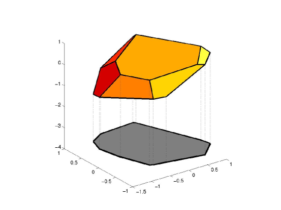
Figure 1: A shadow of a polytope

3.1 Formal Description

Our description of the shadow vertex simplex method will be facilitated by the following definition:

Definition 3.1.1 (optVert).

Given vectors $\boldsymbol{\mathit{z}}$, $\boldsymbol{\mathit{a}}_{1},\ldots,\boldsymbol{\mathit{a}}_{n}$ in ${\rm I\kern-2.0ptR}^{d}$ and $\boldsymbol{\mathit{y}}\in{\rm I\kern-2.0ptR}^{n}$, we define $\mbox{\bf optVert}_{\boldsymbol{\mathit{z}}}{\left(\boldsymbol{\mathit{a}}_{1},\ldots,\boldsymbol{\mathit{a}}_{n};\boldsymbol{\mathit{y}}\right)}$ to be the set of $\boldsymbol{\mathit{x}}$ solving

maximize $$\boldsymbol{\mathit{z}}^{T}\boldsymbol{\mathit{x}}$$

subject to $$\left<\boldsymbol{\mathit{a}}_{i}|\boldsymbol{\mathit{x}}\right>\leq y_{i},\mbox{ for $1\leq i\leq n$}.$$

If there are no such $\boldsymbol{\mathit{x}}$, either because the program is unbounded or infeasible, we let $\mbox{\bf optVert}_{\boldsymbol{\mathit{z}}}{\left(\boldsymbol{\mathit{a}}_{1},\ldots,\boldsymbol{\mathit{a}}_{n};\boldsymbol{\mathit{y}}\right)}$ be $\emptyset$. When $\boldsymbol{\mathit{a}}_{1},\ldots,\boldsymbol{\mathit{a}}_{n}$ and $\boldsymbol{\mathit{y}}$ are understood, we will use the notation $\mbox{\bf optVert}_{\boldsymbol{\mathit{z}}}$.

We note that, for linear programs in general position, $\mbox{\bf optVert}_{\boldsymbol{\mathit{z}}}$ will either be empty or contain one vertex.

Using this definition, we will give a description of the shadow vertex method assuming that a vertex $\boldsymbol{\mathit{x}}_{0}$ and a vector $\boldsymbol{\mathit{t}}$ are known for which $\mbox{\bf optVert}_{\boldsymbol{\mathit{t}}}=\boldsymbol{\mathit{x}}_{0}$. An algorithm that works without this assumption will be described in Section 3.3. Given $\boldsymbol{\mathit{t}}$ and $\boldsymbol{\mathit{z}}$, we define objective functions interpolating between the two by

$$\boldsymbol{\mathit{q}}_{\lambda}=(1-\lambda)\boldsymbol{\mathit{t}}+\lambda\boldsymbol{\mathit{z}}.$$

The shadow-vertex method will proceed by varying $\lambda$ from $0$ to $1$, and tracking $\mbox{\bf optVert}_{\boldsymbol{\mathit{q}}_{\lambda}}$. We will denote the vertices encountered by $\boldsymbol{\mathit{x}}_{0},\boldsymbol{\mathit{x}}_{1},\dots,\boldsymbol{\mathit{x}}_{k}$, and we will set $\lambda_{i}$ so that $\boldsymbol{\mathit{x}}_{i}\in\mbox{\bf optVert}_{\boldsymbol{\mathit{q}}_{\lambda}}$ for $\lambda\in[\lambda_{i},\lambda_{i+1}]$.

As our main motivation for presenting the primal algorithm is to develop intuition in the reader, we will not dwell on issues of degeneracy in its description. We will present a polar version of this algorithm with a proof of correctness in the next section.

primal shadow-vertex method
Input: $\boldsymbol{\mathit{a}}_{1},\ldots,\boldsymbol{\mathit{a}}_{n}$, $\boldsymbol{\mathit{y}}$, $\boldsymbol{\mathit{z}}$, and $\boldsymbol{\mathit{x}}_{0}$ and $\boldsymbol{\mathit{t}}$ satisfying $\left\{\boldsymbol{\mathit{x}}_{0}\right\}=\mbox{\bf optVert}_{\boldsymbol{\mathit{t}}}{\left(\boldsymbol{\mathit{a}}_{1},\ldots,\boldsymbol{\mathit{a}}_{n};\boldsymbol{\mathit{y}}\right)}$. (1) Set $\lambda_{0}=0$, and $i=0$. (2) Set $\lambda_{1}$ to be maximal such that $\left\{\boldsymbol{\mathit{x}}_{0}\right\}=\mbox{\bf optVert}_{\boldsymbol{\mathit{q}}_{\lambda}}$ for $\lambda\in[\lambda_{0},\lambda_{1}]$. (3) while $\lambda_{i+1}<1$, (a) Set $i=i+1$. (b) Find an $\boldsymbol{\mathit{x}}_{i}$ for which there exists a $\lambda_{i+1}>\lambda_{i}$ such that $\boldsymbol{\mathit{x}}_{i}\in\mbox{\bf optVert}_{\boldsymbol{\mathit{q}}_{\lambda}}$ for $\lambda\in[\lambda_{i},\lambda_{i+1}]$. If no such $\boldsymbol{\mathit{x}}_{i}$ exists, return unbounded. (c) Let $\lambda_{i+1}$ be maximal such that $\boldsymbol{\mathit{x}}_{i}\in\mbox{\bf optVert}_{\boldsymbol{\mathit{q}}_{\lambda}}$ for $\lambda\in[\lambda_{i},\lambda_{i+1}]$. (4) return $\boldsymbol{\mathit{x}}_{i}$.

Step $(b)$ of this algorithm deserves further explanation. Assuming that the linear program is in general position with respect to $\boldsymbol{\mathit{t}}$, each vertex $\boldsymbol{\mathit{x}}_{i}$ will have exactly $d$ neighbors, and the vertex $\boldsymbol{\mathit{x}}_{i+1}$ will be one of these [Bor80, Lemma 1.3]. Thus, the algorithm can be described as a simplex method. While one could implement the method by examining these $d$ vertices in turn, more efficient implementations are possible. For an efficient implementation of this algorithm in tableau form, we point the reader to the exposition in [Bor80, Section 1.3].

3.2 Polar Description

Following Borgwardt [Bor80], we will analyze the shadow vertex method from a polar perspective. This polar perspective is natural provided that all $y_{i}>0$. In this section, we will describe a polar variant of the shadow-vertex method that works under this assumption. In the next section, we will describe a two-phase shadow vertex method that uses this polar variant to solve linear programs with arbitrary $y_{i}$s.

While it is not strictly necessary for the results in this paper, we remind the reader that for a polytope $P=\left\{\boldsymbol{\mathit{x}}:\left<\boldsymbol{\mathit{x}}|\boldsymbol{\mathit{a}}_{i}\right>\leq 1,\forall i\right\}$, the polar of $P$ is $\left\{\boldsymbol{\mathit{y}}:\left<\boldsymbol{\mathit{x}}|\boldsymbol{\mathit{y}}\right>\leq 1,\forall\boldsymbol{\mathit{x}}\in P\right\}$. An equivalent definition of the polar is $\mbox{{ConvHull}}\left(\mathbf{0},\boldsymbol{\mathit{a}}_{1},\ldots,\boldsymbol{\mathit{a}}_{n}\right)$. We remark that $P$ is bounded if and only if $\mathbf{0}$ is in the interior of $\mbox{{ConvHull}}\left(\boldsymbol{\mathit{a}}_{1},\ldots,\boldsymbol{\mathit{a}}_{n}\right)$. The polar motivates:

Figure 2: In example (a), $\mathrm{optSimp}=\left\{\left\{\boldsymbol{\mathit{a}}_{1},\boldsymbol{\mathit{a}}_{2},\boldsymbol{\mathit{a}}_{3}\right\}\right\}$. In example (b), $\mathrm{optSimp}=\left\{\left\{\boldsymbol{\mathit{a}}_{1},\boldsymbol{\mathit{a}}_{2},\boldsymbol{\mathit{a}}_{3}\right\},\left\{\boldsymbol{\mathit{a}}_{2},\boldsymbol{\mathit{a}}_{3},\boldsymbol{\mathit{a}}_{4}\right\}\right\}$. In example (c), $\mathrm{optSimp}=\emptyset$,

Definition 3.2.1 (optSimp).

For $\boldsymbol{\mathit{z}}$ and $\boldsymbol{\mathit{a}}_{1},\ldots,\boldsymbol{\mathit{a}}_{n}$ in ${\rm I\kern-2.0ptR}^{d}$ and $\boldsymbol{\mathit{y}}\in{\rm I\kern-2.0ptR}^{n}$, $y_{i}>0$, we let $\mbox{\bf optSimp}_{\boldsymbol{\mathit{z}}}{\left(\boldsymbol{\mathit{a}}_{1},\ldots,\boldsymbol{\mathit{a}}_{n};\boldsymbol{\mathit{y}}\right)}$ denote the set of $I\in\binom{[n]}{d}$ such that $\boldsymbol{\mathit{A}}_{I}$ has full rank, $\bigtriangleup\left((\boldsymbol{\mathit{a}}_{i}/y_{i})_{i\in I}\right)$ is a facet of $\mbox{{ConvHull}}\left(\mathbf{0},\boldsymbol{\mathit{a}}_{1}/y_{1},\ldots,\boldsymbol{\mathit{a}}_{n}/y_{n}\right)$ and $\boldsymbol{\mathit{z}}\in\mbox{{\bf Cone}}\left((\boldsymbol{\mathit{a}}_{i})_{i\in I}\right)$. When $\boldsymbol{\mathit{y}}$ is understood to be $\mathbf{1}$, we will use the notation $\mbox{\bf optSimp}_{\boldsymbol{\mathit{z}}}{\left(\boldsymbol{\mathit{a}}_{1},\ldots,\boldsymbol{\mathit{a}}_{n}\right)}$ When $\boldsymbol{\mathit{a}}_{1},\ldots,\boldsymbol{\mathit{a}}_{n}$ and $\boldsymbol{\mathit{y}}$ are understood, we will use the notation $\mbox{\bf optSimp}_{\boldsymbol{\mathit{z}}}$.

We remark that for $\boldsymbol{\mathit{y}}$, $\boldsymbol{\mathit{z}}$ and $\boldsymbol{\mathit{a}}_{1},\ldots,\boldsymbol{\mathit{a}}_{n}$ in general position, $\mbox{\bf optSimp}_{\boldsymbol{\mathit{z}}}{\left(\boldsymbol{\mathit{a}}_{1},\ldots,\boldsymbol{\mathit{a}}_{n};\boldsymbol{\mathit{y}}\right)}$ will be the empty set or contain just one set of indices $I$.

The following proposition follows from the duality theory of linear programming:

Proposition 3.2.2 (Duality).

For $y_{1},\ldots,y_{n}>0$, $I\in\mbox{\bf optSimp}_{\boldsymbol{\mathit{z}}}{\left(\boldsymbol{\mathit{a}}_{1}/y_{1},\ldots,\boldsymbol{\mathit{a}}_{n}/y_{n}\right)}$ if and only if there exists an $\boldsymbol{\mathit{x}}$ such that $\boldsymbol{\mathit{x}}\in\mbox{\bf optVert}_{\boldsymbol{\mathit{z}}}{\left(\boldsymbol{\mathit{a}}_{1},\ldots,\boldsymbol{\mathit{a}}_{n};\boldsymbol{\mathit{y}}\right)}$ and $\left<\boldsymbol{\mathit{x}}|\boldsymbol{\mathit{a}}_{i}\right>=y_{i}$, for $i\in I$.

We now state the polar shadow vertex method.

polar shadow-vertex method
Input: • $\boldsymbol{\mathit{a}}_{1},\ldots,\boldsymbol{\mathit{a}}_{n}$, $\boldsymbol{\mathit{z}}$, and $y_{1},\ldots,y_{n}>0$, • $I\in\binom{[n]}{d}$ and $\boldsymbol{\mathit{t}}$ satisfying $I\in\mbox{\bf optSimp}_{\boldsymbol{\mathit{t}}}{\left(\boldsymbol{\mathit{a}}_{1}/y_{1},\ldots,\boldsymbol{\mathit{a}}_{n}/y_{n}\right)}$. (1) Set $\lambda_{0}=0$ and $i=0$. (2) Set $\lambda_{1}$ to be maximal such that for $\lambda\in[\lambda_{0},\lambda_{1}]$, $$I\in\mbox{\bf optSimp}_{\boldsymbol{\mathit{q}}_{\lambda}}{\left(\boldsymbol{\mathit{a}}_{1}/y_{1},\ldots,\boldsymbol{\mathit{a}}_{n}/y_{n}\right)}.$$ (3) while $\lambda_{i+1}<1$, (a) Set $i=i+1$. (b) Find a $j$ and $k$ for which there exists a $\lambda_{i+1}>\lambda_{i}$ such that $$I\cup\left\{j\right\}-\left\{k\right\}\in\mbox{\bf optSimp}_{\boldsymbol{\mathit{q}}_{\lambda}}{\left(\boldsymbol{\mathit{a}}_{1}/y_{1},\ldots,\boldsymbol{\mathit{a}}_{n}/y_{n}\right)}$$ for $\lambda\in[\lambda_{i},\lambda_{i+1}]$. If no such $j$ and $k$ exist, return unbounded. (c) Set $I=I\cup\left\{j\right\}-\left\{k\right\}$. (d) Let $\lambda_{i+1}$ be maximal such that $I\in\mbox{\bf optSimp}_{\boldsymbol{\mathit{t}}}{\left(\boldsymbol{\mathit{a}}_{1}/y_{1},\ldots,\boldsymbol{\mathit{a}}_{n}/y_{n}\right)}$ for $\lambda\in[\lambda_{i},\lambda_{i+1}]$. (4) return $I$.

The $\boldsymbol{\mathit{x}}$ optimizing the linear program, namely $\mbox{\bf optVert}_{\boldsymbol{\mathit{z}}}{\left(\boldsymbol{\mathit{a}}_{1},\ldots,\boldsymbol{\mathit{a}}_{n};\boldsymbol{\mathit{y}}\right)}$, is given by the equations $\left<\boldsymbol{\mathit{x}}|\boldsymbol{\mathit{a}}_{i}\right>=y_{i}$, for $i\in I$.

Borgwardt [Bor80, Lemma 1.9] establishes that such $j$ and $k$ can be found in step $(b)$ if there exists an $\epsilon$ for which $\mbox{\bf optSimp}_{\boldsymbol{\mathit{q}}_{\lambda_{i}+\epsilon}}{\left(\boldsymbol{\mathit{a}}_{1}/y_{1},\ldots,\boldsymbol{\mathit{a}}_{n}/y_{n}\right)}\not=\emptyset$. That the algorithm may conclude that the program is unbounded if a $j$ and $k$ cannot be found in step $(b)$ follows from:

Proposition 3.2.3 (Detecting unbounded programs).

If there is an $i$ and an $\epsilon>0$ such that $\lambda_{i}+\epsilon<1$ and $\mbox{\bf optSimp}_{\boldsymbol{\mathit{q}}_{\lambda_{i}+\epsilon}}{\left(\boldsymbol{\mathit{a}}_{1}/y_{1},\ldots,\boldsymbol{\mathit{a}}_{n}/y_{n}\right)}=\emptyset$, then $\mbox{\bf optSimp}_{\boldsymbol{\mathit{z}}}{\left(\boldsymbol{\mathit{a}}_{1}/y_{1},\ldots,\boldsymbol{\mathit{a}}_{n}/y_{n}\right)}=\emptyset$.

Proof.

$\mbox{\bf optSimp}_{\boldsymbol{\mathit{q}}_{\lambda_{i}+\epsilon}}{\left(\boldsymbol{\mathit{a}}_{1}/y_{1},\ldots,\boldsymbol{\mathit{a}}_{n}/y_{n}\right)}=\emptyset$ if and only if $\boldsymbol{\mathit{q}}_{\lambda_{i}+\epsilon}\not\in\mbox{{\bf Cone}}\left(\boldsymbol{\mathit{a}}_{1},\ldots,\boldsymbol{\mathit{a}}_{n}\right)$. The proof now follows from the facts that $\mbox{{\bf Cone}}\left(\boldsymbol{\mathit{a}}_{1},\ldots,\boldsymbol{\mathit{a}}_{n}\right)$ is a convex set and $\boldsymbol{\mathit{q}}_{\lambda_{i}+\epsilon}$ is a positive multiple of a convex combination of $\boldsymbol{\mathit{t}}$ and $\boldsymbol{\mathit{z}}$.

The running time of the shadow-vertex method is bounded by the number of vertices in shadow of the polytope defined by the constraints of the linear program. Formally, this is

Definition 3.2.4 (Shadow).

For independent vectors $\boldsymbol{\mathit{t}}$ and $\boldsymbol{\mathit{z}}$, $\boldsymbol{\mathit{a}}_{1},\ldots,\boldsymbol{\mathit{a}}_{n}$ in ${\rm I\kern-2.0ptR}^{d}$ and $\boldsymbol{\mathit{y}}\in{\rm I\kern-2.0ptR}^{n}$, $\boldsymbol{\mathit{y}}>0$,

$$\mbox{{\bf Shadow}}_{\boldsymbol{\mathit{t}},\boldsymbol{\mathit{z}}}\left(\boldsymbol{\mathit{a}}_{1},\ldots,\boldsymbol{\mathit{a}}_{n};\boldsymbol{\mathit{y}}\right)\stackrel{{\scriptstyle\mathrm{def}}}{{=}}\bigcup_{\boldsymbol{\mathit{q}}\in\textbf{Span}\left(\boldsymbol{\mathit{t}},\boldsymbol{\mathit{z}}\right)}\left\{\mbox{\bf optSimp}_{\boldsymbol{\mathit{q}}}{\left(\boldsymbol{\mathit{a}}_{1}/y_{1},\ldots,\boldsymbol{\mathit{a}}_{n}/y_{n}\right)}\right\}.$$

If $\boldsymbol{\mathit{y}}$ is understood to be $\mathbf{1}$, we will just write $\mbox{{\bf Shadow}}_{\boldsymbol{\mathit{t}},\boldsymbol{\mathit{z}}}\left(\boldsymbol{\mathit{a}}_{1},\ldots,\boldsymbol{\mathit{a}}_{n}\right)$.

3.3 Two-Phase Method

We now describe a two-phase shadow vertex method that solves linear programs of form

maximize $$\left<\boldsymbol{\mathit{z}}|\boldsymbol{\mathit{x}}\right>$$

subject to $$\left<\boldsymbol{\mathit{a}}_{i}|\boldsymbol{\mathit{x}}\right>\leq y_{i},\mbox{ for $1\leq i\leq n$}. (LP)$$

There are three issues that we must resolve before we can apply the polar shadow vertex method as described in Section 3.2 to the solution of such programs:

1. the method must know a feasible vertex of the linear program,

2. the linear program might not even be feasible, and

3. some $y_{i}$ might be non-positive.

The first two issues are standard motivations for two-phase methods, while the third is motivated by the polar perspective from which we prefer to analyze the shadow vertex method. We resolve these issues in two stages. We first relax the constraints of $LP$ to construct a linear program $LP^{\prime}$ such that

1. the right-hand vector of the linear program is positive, and

2. we know a feasible vertex of the linear program.

After solving $LP^{\prime}$, we construct another linear program, $LP^{+}$, in one higher dimension that interpolates between $LP$ and $LP^{\prime}$. $LP^{+}$ has properties $(a)$ and $(b)$, and we can use the shadow vertex method on $LP^{+}$ to transform the solution to $LP^{\prime}$ into a solution of $LP$.

Our two-phase method first chooses a $d$-set $I$ to define the known feasible vertex of $LP^{\prime}$. The linear program $LP^{\prime}$ is determined by $\boldsymbol{\mathit{A}}$, $\boldsymbol{\mathit{z}}$ and the choice of $I$. However, the magnitude of the right-hand entries in $LP^{\prime}$ depends upon $\mbox{\bf s}_{\textbf{min}}\left(A_{I}\right)$. To reduce the chance that these entries will need to be large, we examine several randomly chosen $d$-sets, and use the one maximizing $\mbox{\bf s}_{\textbf{min}}$.

The algorithm then sets

$$M =2^{\left\lceil\lg\left(\max_{i}\left\|y_{i},\boldsymbol{\mathit{a}}_{i}\right\|\right)\right\rceil+2},$$

$$\kappa =2^{\left\lfloor\lg\left(\mbox{\bf s}_{\textbf{min}}\left(\boldsymbol{\mathit{A}}_{I}\right)\right)\right\rfloor},\text{and}$$

$$y_{i}^{\prime} =\begin{cases}M&\text{for $i\in I$}\\ \sqrt{d}M^{2}/4\kappa&\text{otherwise.}\end{cases}$$

These define the program $LP^{\prime}$:

maximize $$\left<\boldsymbol{\mathit{z}}|\boldsymbol{\mathit{x}}\right>$$

subject to $$\left<\boldsymbol{\mathit{a}}_{i}|\boldsymbol{\mathit{x}}\right>\leq y^{\prime}_{i},\mbox{ for $1\leq i\leq n$}. (LP^{\prime})$$

By Proposition 3.3.1, $\boldsymbol{\mathit{A}}_{I}$ is a feasible basis for $LP^{\prime}$, and optimizes any objective function of the form $\boldsymbol{\mathit{A}}_{I}\boldsymbol{\alpha}$, for $\boldsymbol{\alpha}>0$. Our two-phase algorithm will solve $LP^{\prime}$ by starting the polar shadow-vertex algorithm at the basis $I$ and the objective function $\boldsymbol{\mathit{A}}_{I}\boldsymbol{\alpha}$ for a randomly chosen $\boldsymbol{\alpha}$ satisfying $\sum\alpha_{i}=1$ and $\alpha_{i}\geq 1/d^{2}$, for all $i$.

Proposition 3.3.1 (Initial simplex of $LP^{\prime}$).

For any $\boldsymbol{\alpha}>0$, $I=\mbox{\bf optSimp}_{\boldsymbol{\mathit{A}}_{I}\boldsymbol{\alpha}}{\left(\boldsymbol{\mathit{a}}_{1},\ldots,\boldsymbol{\mathit{a}}_{n};\boldsymbol{\mathit{y}}^{\prime}\right)}$.

Proof.

Let $\boldsymbol{\mathit{x}}^{\prime}$ be the solution of the linear system

$$\left<\boldsymbol{\mathit{a}}_{i}|\boldsymbol{\mathit{x}}^{\prime}\right>=y^{\prime}_{i},\qquad\mbox{for}\qquad i\in I.$$

By Definition 2.2.3 and Proposition 2.2.4 (a),

$$\left\|\boldsymbol{\mathit{x}}^{\prime}\right\|\leq\left\|\boldsymbol{\mathit{y}}^{\prime}_{I}\right\|\left\|\boldsymbol{\mathit{A}}_{I}^{-1}\right\|\leq M\sqrt{d}\left\|\boldsymbol{\mathit{A}}_{I}^{-1}\right\|=M\sqrt{d}/\mbox{\bf s}_{\textbf{min}}\left(\boldsymbol{\mathit{A}}_{I}\right).$$

So, for all $i\not\in I$,

$$\left<\boldsymbol{\mathit{a}}_{i}|\boldsymbol{\mathit{x}}^{\prime}\right>\leq(\max_{i}\left\|\boldsymbol{\mathit{a}}_{i}\right\|)M\sqrt{d}/\mbox{\bf s}_{\textbf{min}}\left(\boldsymbol{\mathit{A}}_{I}\right)<M^{2}\sqrt{d}/4\kappa.$$

Thus, for all $i\not\in I$,

$$\left<\boldsymbol{\mathit{a}}_{i}|\boldsymbol{\mathit{x}}^{\prime}\right><y^{\prime}_{i},$$

and, by Definition 3.2.1, $I=\mbox{\bf optSimp}_{\boldsymbol{\mathit{A}}_{I}\boldsymbol{\alpha}}{\left(\boldsymbol{\mathit{a}}_{1},\ldots,\boldsymbol{\mathit{a}}_{n};\boldsymbol{\mathit{y}}^{\prime}\right)}$.

We will now define a linear program $LP^{+}$ that interpolates between $LP^{\prime}$ and $LP$. This linear program will contain an extra variable $x_{0}$ and constraints of the form

$$\left<\boldsymbol{\mathit{a}}_{i}|\boldsymbol{\mathit{x}}\right>\leq\left(\frac{1+x_{0}}{2}\right)y_{i}+\left(\frac{1-x_{0}}{2}\right)y^{\prime}_{i},$$

and $-1\leq x_{0}\leq 1$. So, for $x_{0}=1$ we see the original program $LP$ while for $x_{0}=-1$ we get $LP^{\prime}$. Formally, we let

$$\boldsymbol{\mathit{a}}^{+}_{i} =\left\{\begin{array}[]{ll}\left((y^{\prime}_{i}-y_{i})/2,\boldsymbol{\mathit{a}}_{i}\right)&\text{ for $1\leq i\leq n$}\\ \left(1,0,\ldots,0\right)&\text{ for $i=0$}\\ \left(-1,0,\ldots,0\right)&\text{ for $i=-1$}\end{array}\right.$$

$$y^{+}_{i} =\left\{\begin{array}[]{ll}(y^{\prime}_{i}+y_{i})/2&\text{ for $1\leq i\leq n$}\\ 1&\text{ for $i=0$}\\ 1&\text{ for $i=-1$}\end{array}\right.$$

$$\boldsymbol{\mathit{z}}^{+} =(1,0,\ldots,0),$$

and we define $LP^{+}$ by

maximize $$\left<\boldsymbol{\mathit{z}}^{+}|(x_{0},\boldsymbol{\mathit{x}})\right>$$

subject to $$\left<\boldsymbol{\mathit{a}}^{+}_{i}|(x_{0},\boldsymbol{\mathit{x}})\right>\leq y^{+}_{i},\mbox{ for $-1\leq i\leq n$}, (LP^{+})$$

and we set

$$\boldsymbol{\mathit{y}}^{+}\stackrel{{\scriptstyle\mathrm{def}}}{{=}}(y^{+}_{-1},\ldots,y^{+}_{n}).$$

By Proposition 3.3.2, $\sqrt{d}M/4\kappa\geq 1$, so $y^{\prime}_{i}\geq M$ and $y^{+}_{i}>0$, for all $i$. If $LP$ is infeasible, then the solution to $LP^{+}$ will have $x_{0}<1$. If $LP$ is feasible, then the solution to $LP^{+}$ will have form $(1,\boldsymbol{\mathit{x}})$ where $\boldsymbol{\mathit{x}}$ is a feasible point for $LP$. If we use the shadow-vertex method to solve $LP^{+}$ starting from the appropriate initial vector, then $\boldsymbol{\mathit{x}}$ will be an optimal solution to $LP$.

Proposition 3.3.2 (relation of $M$ and $\kappa$).

For $M$ and $\kappa$ as set by the algorithm, $\sqrt{d}M/4\kappa\geq 1$.

Proof.

By definition, $\kappa\leq\mbox{\bf s}_{\textbf{min}}\left(\boldsymbol{\mathit{A}}_{I}\right)$. On the other hand, $\mbox{\bf s}_{\textbf{min}}\left(\boldsymbol{\mathit{A}}_{I}\right)\leq\left\|\boldsymbol{\mathit{A}}_{I}\right\|\leq\sqrt{d}\max_{i}\left\|\boldsymbol{\mathit{a}}_{i}\right\|$, by Proposition 2.2.4 (d). Finally, $M\geq 4\max_{i}\left\|\boldsymbol{\mathit{a}}_{i}\right\|$.

We now state and prove the correctness of the two-phase shadow vertex method.

two-phase shadow-vertex method
Input: $\boldsymbol{\mathit{A}}=\left(\boldsymbol{\mathit{a}}_{1},\ldots,\boldsymbol{\mathit{a}}_{n}\right)$, $\boldsymbol{\mathit{y}}$, $\boldsymbol{\mathit{z}}$. (1) Let $\mathcal{I}=\left\{I_{1},\ldots,I_{3nd\ln n}\right\}$ be a collection of randomly chosen sets in $\binom{[n]}{d}$, and let $I\in\mathcal{I}$ be the set maximizing $\mbox{\bf s}_{\textbf{min}}\left(\boldsymbol{\mathit{A}}_{I}\right)$. (2) Set $M=2^{\left\lceil\lg\left(\max_{i}\left\|y_{i},\boldsymbol{\mathit{a}}_{i}\right\|\right)\right\rceil+2}$ and $\kappa=2^{\left\lfloor\lg\left(\mbox{\bf s}_{\textbf{min}}\left(\boldsymbol{\mathit{A}}_{I}\right)\right)\right\rfloor}$. (3) Set $y_{i}^{\prime}=\begin{cases}M&\text{for $i\in I$}\\ \sqrt{d}M^{2}/4\kappa&\text{otherwise.}\end{cases}$. (4) Choose $\boldsymbol{\alpha}$ uniformly at random from $\left\{\boldsymbol{\alpha}:\sum\alpha_{i}=1\text{ and }\alpha_{i}\geq 1/d^{2}\right\}$. Set $\boldsymbol{\mathit{t}}^{\prime}=\boldsymbol{\mathit{A}}_{I}\boldsymbol{\alpha}$. (5) Let $J$ be the output of the polar shadow vertex algorithm on $LP^{\prime}$ on input $I$ and $\boldsymbol{\mathit{t}}^{\prime}$. If $LP^{\prime}$ is unbounded, then return unbounded. (6) Let $\zeta>0$ be such that $$\left\{-1\right\}\cup J\in\mbox{\bf optSimp}_{(-\zeta,\boldsymbol{\mathit{z}})}{\left(\boldsymbol{\mathit{a}}^{+}_{-1}/y^{+}_{-1},\ldots,\boldsymbol{\mathit{a}}^{+}_{n}/y^{+}_{n}\right)}.$$ (7) Let $K$ be the output of the polar shadow vertex algorithm on $LP^{+}$ on input $\left\{-1\right\}\cup J$, $(-\zeta,\boldsymbol{\mathit{z}})$. (8) Compute $(x_{0},\boldsymbol{\mathit{x}})$ satisfying $\left<(x_{0},\boldsymbol{\mathit{x}})|\boldsymbol{\mathit{a}}^{+}_{i}\right>=y_{i}$ for $i\in K$. (9) If $x_{0}<1$, return infeasible. Otherwise, return $\boldsymbol{\mathit{x}}$.

The following propositions prove the correctness of the algorithm.

Proposition 3.3.3 (Unbounded programs).

The following are equivalent

1. $LP$ is unbounded;

2. $LP^{\prime}$ is unbounded;

3. there exists a $1>\lambda>0$ such that $\mbox{\bf optSimp}_{\lambda(1,\mathbf{0})+(1-\lambda)(-\zeta,\boldsymbol{\mathit{z}})}{\left(\boldsymbol{\mathit{a}}^{+}_{-1},\ldots,\boldsymbol{\mathit{a}}^{+}_{n};\boldsymbol{\mathit{y}}^{+}\right)}=\emptyset$;

4. for all $1>\lambda>0$, $\mbox{\bf optSimp}_{\lambda(1,\mathbf{0})+(1-\lambda)(-\zeta,\boldsymbol{\mathit{z}})}{\left(\boldsymbol{\mathit{a}}^{+}_{-1},\ldots,\boldsymbol{\mathit{a}}^{+}_{n};\boldsymbol{\mathit{y}}^{+}\right)}=\emptyset$.

Proposition 3.3.4 (Bounded programs).

If $LP^{\prime}$ is bounded and has solution $J$, then

1. there exists $\zeta_{0}$ such that for all $\zeta>\zeta_{0}$, $\left\{-1\right\}\cup J\in\mbox{\bf optSimp}_{(-\zeta,\boldsymbol{\mathit{z}})}{\left(\boldsymbol{\mathit{a}}^{+}_{-1},\ldots,\boldsymbol{\mathit{a}}^{+}_{n};\boldsymbol{\mathit{y}}^{+}\right)}$,

2. If $LP$ is feasible, then for $K^{\prime}\in\mbox{\bf optSimp}_{\boldsymbol{\mathit{z}}}{\left(\boldsymbol{\mathit{a}}_{1},\ldots,\boldsymbol{\mathit{a}}_{n};\boldsymbol{\mathit{y}}\right)}$, there exists $\xi_{0}$ such that for all $\xi>\xi_{0}$, $\left\{0\right\}\cup K^{\prime}\in\mbox{\bf optSimp}_{(\xi,\boldsymbol{\mathit{z}})}{\left(\boldsymbol{\mathit{a}}^{+}_{-1},\ldots,\boldsymbol{\mathit{a}}^{+}_{n};\boldsymbol{\mathit{y}}^{+}\right)}$, and

3. if we use the shadow vertex method to solve $LP^{+}$ starting from $\left\{-1,J\right\}$ and objective function $(-\zeta,\boldsymbol{\mathit{z}})$, then the output of the algorithm will have form $\left\{0\right\}\cup K^{\prime}$, where $K^{\prime}$ is a solution to $LP$.

Proof of Proposition 3.3.3    $LP$ is unbounded if and only if there exists a vector $\boldsymbol{\mathit{v}}$ such that $\left<\boldsymbol{\mathit{z}}|\boldsymbol{\mathit{v}}\right>>0$ and $\left<\boldsymbol{\mathit{a}}_{i}|\boldsymbol{\mathit{v}}\right>\leq 0$ for all $i$. The same holds for $LP^{\prime}$, and establishes the equivalence of $(a)$ and $(b)$. To show that $(a)$ or $(b)$ implies $(d)$, observe

$$\left<\lambda(1,\mathbf{0})+(1-\lambda)(-\zeta,\boldsymbol{\mathit{z}})|(0,\boldsymbol{\mathit{v}})\right> =(1-\lambda)\left<\boldsymbol{\mathit{z}}|\boldsymbol{\mathit{v}}\right>>0,$$ (8)

$$\left<\boldsymbol{\mathit{a}}^{+}_{i}|(0,\boldsymbol{\mathit{v}})\right> =\left<\boldsymbol{\mathit{a}}_{i}|\boldsymbol{\mathit{v}}\right>,\text{ for $i=1,\ldots,n,$}$$ (9)

$$\left<\boldsymbol{\mathit{a}}_{0}^{+}|(0,\boldsymbol{\mathit{v}})\right> =0,\text{ and}$$

$$\left<\boldsymbol{\mathit{a}}_{-1}^{+}|(0,\boldsymbol{\mathit{v}})\right> =0.$$

To show that $(c)$ implies $(a)$ and $(b)$, note that $\boldsymbol{\mathit{a}}^{+}_{0}$ and $\boldsymbol{\mathit{a}}^{+}_{-1}$ are arranged so that if for some $v_{0}$ we have

$$\left<\boldsymbol{\mathit{a}}^{+}_{i}|(v_{0},\boldsymbol{\mathit{v}})\right>\leq 0,\text{ for $-1\leq i\leq n$},$$

then $v_{0}=0$. This identity allows us to apply (8) and (9) to show $(c)$ implies $(a)$ and $(b)$.

Proof of Proposition 3.3.4    Let $J$ be the solution to $LP^{\prime}$ and let $\boldsymbol{\mathit{x}}^{\prime}=\boldsymbol{\mathit{A}}_{J}^{-1}\boldsymbol{\mathit{y}}^{\prime}_{J}$ be the corresponding vertex. We then have

$$\left<\boldsymbol{\mathit{x}}^{\prime}|\boldsymbol{\mathit{a}}_{i}\right> =y^{{}^{\prime}}_{i}, i\in J$$ for , and

$$\left<\boldsymbol{\mathit{x}}^{\prime}|\boldsymbol{\mathit{a}}_{i}\right> \leq y^{{}^{\prime}}_{i}, \text{ for $i\not\in J$}.$$

Therefore, it is clear that

$$\left<(-1,\boldsymbol{\mathit{x}}^{\prime})|\boldsymbol{\mathit{a}}^{+}_{i}\right> =y^{+}_{i}, i\in\left\{-1\right\}\cup J$$ for , and

$$\left<(-1,\boldsymbol{\mathit{x}}^{\prime})|\boldsymbol{\mathit{a}}^{+}_{i}\right> \leq y^{+}_{i}, \text{ for $i\not\in\left\{-1\right\}\cup J$}.$$

Thus, $\bigtriangleup\left(\boldsymbol{\mathit{a}}^{+}_{-1},(\boldsymbol{\mathit{a}}^{+}_{i})_{i\in J}\right)$ is a facet of $LP^{+}$. To see that there exists a $\zeta_{0}$ such that it optimizes $(-\zeta,\boldsymbol{\mathit{z}})$ for all $\zeta>\zeta_{0}$, first observe that there exist $\alpha_{i}>0$, for $i\in J$, such that $\sum_{i\in J}\alpha_{i}\boldsymbol{\mathit{a}}_{i}=\boldsymbol{\mathit{z}}$. Now, let $(-\zeta_{0},\boldsymbol{\mathit{z}})=\sum_{i\in J}\alpha_{i}\boldsymbol{\mathit{a}}^{+}_{i}$. For $\zeta>\zeta_{0}$, we have

$$(-\zeta,\boldsymbol{\mathit{z}})=(\zeta-\zeta_{0})\boldsymbol{\mathit{a}}^{+}_{-1}+\sum_{i\in J}\alpha_{i}\boldsymbol{\mathit{a}}^{+}_{i},$$

which proves $(-\zeta,\boldsymbol{\mathit{z}})\in\mbox{{\bf Cone}}\left(\boldsymbol{\mathit{a}}^{+}_{-1},(\boldsymbol{\mathit{a}}^{+}_{i})_{i\in J}\right)$ and completes the proof of $(a)$.

The proof of $(b)$ is similar.

To prove part $(c)$, let $K$ be as in step $(7)$. Then, there exists a $\lambda_{k}$ such that for all $\lambda\in(\lambda_{k},1)$,

$$K=\mbox{\bf optSimp}_{(1-\lambda)(-\zeta,\boldsymbol{\mathit{z}})+\lambda\boldsymbol{\mathit{z}}^{+}}{\left(\boldsymbol{\mathit{a}}^{+}_{-1},\ldots,\boldsymbol{\mathit{a}}^{+}_{n};\boldsymbol{\mathit{y}}^{+}\right)}.$$

Let $(x_{0},\boldsymbol{\mathit{x}})$ satisfy $\left<(x_{0},\boldsymbol{\mathit{x}})|\boldsymbol{\mathit{a}}^{+}_{i}\right>=y^{+}_{i}$, for $i\in K$. Then, by Proposition 3.2.2,

$$(x_{0},\boldsymbol{\mathit{x}})=\mbox{\bf optVert}_{(1-\lambda)(-\zeta,\boldsymbol{\mathit{z}})+\lambda\boldsymbol{\mathit{z}}^{+}}{\left(\boldsymbol{\mathit{a}}^{+}_{-1},\ldots,\boldsymbol{\mathit{a}}^{+}_{n};\boldsymbol{\mathit{y}}^{+}\right)}.$$

If $x_{0}<1$, then LP was infeasible. Otherwise, let $\boldsymbol{\mathit{x}}^{*}=\mbox{\bf optVert}_{\boldsymbol{\mathit{z}}}{\left(\boldsymbol{\mathit{a}}_{1},\ldots,\boldsymbol{\mathit{a}}_{n};\boldsymbol{\mathit{y}}\right)}$. By part $(b)$, there exists $\xi_{0}$ such that for all $\xi>\xi_{0}$,

$$(1,\boldsymbol{\mathit{x}}^{*})=\mbox{\bf optVert}_{(\xi,\boldsymbol{\mathit{z}})}{\left(\boldsymbol{\mathit{a}}^{+}_{-1},\ldots,\boldsymbol{\mathit{a}}^{+}_{n};\boldsymbol{\mathit{y}}^{+}\right)}.$$

For $\xi=-\zeta+\lambda/(1-\lambda)$, we have

$$(\xi,\boldsymbol{\mathit{z}})=\frac{1}{1-\lambda}\left((1-\lambda)(-\zeta,\boldsymbol{\mathit{z}})+\lambda\boldsymbol{\mathit{z}}^{+}\right).$$

So, as $\lambda$ approaches 1, $\xi=-\zeta+\lambda/(1-\lambda)$ goes to infinity and we have

$$\mbox{\bf optVert}_{(1-\lambda)(-\zeta,\boldsymbol{\mathit{z}})+\lambda\boldsymbol{\mathit{z}}^{+}}{\left(\boldsymbol{\mathit{a}}^{+}_{-1},\ldots,\boldsymbol{\mathit{a}}^{+}_{n};\boldsymbol{\mathit{y}}^{+}\right)}=\mbox{\bf optVert}_{(\xi,\boldsymbol{\mathit{z}})}{\left(\boldsymbol{\mathit{a}}^{+}_{-1},\ldots,\boldsymbol{\mathit{a}}^{+}_{n};\boldsymbol{\mathit{y}}^{+}\right)},$$

which implies $(x_{0},\boldsymbol{\mathit{x}})=(1,\boldsymbol{\mathit{x}}^{*})$.

Finally, we bound the number of steps taken in step (7) by the shadow size of a related polytope:

Lemma 3.3.5 (Shadow path of $LP^{+}$).

Let $\boldsymbol{\mathit{a}}^{+}_{-1},\ldots,\boldsymbol{\mathit{a}}^{+}_{n}$ and $y^{+}_{-1},\ldots,y^{+}_{n}$ be as defined in $LP^{+}$. Let $\zeta>0$ be such that $\left\{-1\right\}\cup J=\mbox{\bf optSimp}_{(-\zeta,\boldsymbol{\mathit{z}})}{\left(\boldsymbol{\mathit{a}}^{+}_{-1}/y^{+}_{-1},\ldots,\boldsymbol{\mathit{a}}^{+}_{n}/y^{+}_{n}\right)}$. Then the number of simplex steps made by the polar shadow vertex algorithm while solving $LP^{+}$ from initial basis $\left\{-1\right\}\cup J$ and vector $(-\zeta,\boldsymbol{\mathit{z}})$ is at most

$$2+\left|\mbox{{\bf Shadow}}_{(0,\boldsymbol{\mathit{z}}),\boldsymbol{\mathit{z}}^{+}}\left(\boldsymbol{\mathit{a}}^{+}_{1}/y^{+}_{1},\ldots,\boldsymbol{\mathit{a}}^{+}_{n}/y^{+}_{n}\right)\right|.$$

Proof.

We will establish that $\left\{-1\right\}\in I$ for the first step only. One can similarly prove that $\left\{0\right\}\in I$ is only true at termination.

Let $I\in\mbox{\bf optSimp}_{\boldsymbol{\mathit{q}}_{\lambda}}{\left(\boldsymbol{\mathit{a}}^{+}_{-1}/y^{+}_{-1},\ldots,\boldsymbol{\mathit{a}}^{+}_{n}/y^{+}_{n}\right)}$ have form $\left\{-1\right\}\cup L$. As $\boldsymbol{\mathit{q}}_{0}=\boldsymbol{\mathit{a}}^{+}_{-1}\in\mbox{{\bf Cone}}\left(\boldsymbol{\mathit{A}}_{\left\{-1\right\}\cup L}\right)$, and $\mbox{{\bf Cone}}\left(\boldsymbol{\mathit{A}}_{\left\{-1\right\}\cup L}\right)$ is a convex set, we have $\boldsymbol{\mathit{q}}_{\lambda^{\prime}}\in\mbox{{\bf Cone}}\left(\boldsymbol{\mathit{A}}_{\left\{-1\right\}\cup L}\right)$ for all $0\leq\lambda^{\prime}\leq\lambda$. As $[\lambda_{i},\lambda_{i+1}]$ is exactly the set of $\lambda$ optimized by $\bigtriangleup\left(\boldsymbol{\mathit{A}}_{I}\right)$ in the $i$th step of the polar shadow vertex method, $I$ must be the initial set.

3.4 Discussion

We also note that our analysis of the two-phase algorithm actually takes advantage of the fact that $\kappa$ and $M$ have been set to powers of two. In particular, this fact is used to show that there are not too many likely choices for $\kappa$ and $M$. For the reader who would like to drop this condition, we briefly explain how the argument of Section 5 could be modified to compensate: first, we could consider setting $\kappa$ and $M$ to powers of $1+1/poly(n,d,1/\sigma)$. This would still result in a polynomially bounded number of choices for $\kappa$ and $M$. One could then drop this assumption by observing that allowing $\kappa$ and $M$ to vary in a small range would not introduce too much dependency between the variables.

4 Shadow Size

In this section, we bound the expected size of the shadow of the perturbation of a polytope onto a fixed plane. This is the main geometric result of the paper. The algorithmic results of this paper will rely on extensions of this theorem derived in Section 4.3.

Theorem 4.0.1 (Shadow Size).

Let $d\geq 3$ and $n>d$. Let $\boldsymbol{\mathit{z}}$ and $\boldsymbol{\mathit{t}}$ be independent vectors in ${\rm I\kern-2.0ptR}^{d}$, and let $\mu_{1},\ldots,\mu_{n}$ be Gaussian distributions in ${\rm I\kern-2.0ptR}^{d}$ of standard deviation $\sigma$ centered at points each of norm at most $1$. Then,

$$\operatorname{\textbf{E}}\displaylimits_{\boldsymbol{\mathit{a}}_{1},\ldots,\boldsymbol{\mathit{a}}_{n}}\left[\left|\mbox{{\bf Shadow}}_{\boldsymbol{\mathit{t}},\boldsymbol{\mathit{z}}}\left(\boldsymbol{\mathit{a}}_{1},\ldots,\boldsymbol{\mathit{a}}_{n}\right)\right|\right]\leq\mathcal{D}(n,d,\sigma),$$ (10)

where

$$\mathcal{D}(n,d,\sigma)=\frac{58,888,678\ nd^{3}}{\min\left(\sigma,1/3\sqrt{d\ln n}\right)^{6}},$$

and $\boldsymbol{\mathit{a}}_{1},\ldots,\boldsymbol{\mathit{a}}_{n}$ have density $\prod_{i=1}^{n}\mu_{i}(\boldsymbol{\mathit{a}}_{i})$.

The proof of Theorem 4.0.1, will use the following definitions.

Definition 4.0.2 (ang).

For a vector $\boldsymbol{\mathit{q}}$ and a set $S$, we define

$$\mbox{{\bf ang}}\left(\boldsymbol{\mathit{q}},S\right)=\min_{\boldsymbol{\mathit{x}}\in S}\mbox{{\bf angle}}\left(\boldsymbol{\mathit{q}},\boldsymbol{\mathit{x}}\right),$$

If $S$ is empty, we set $\mbox{{\bf ang}}\left(\boldsymbol{\mathit{q}},\emptyset\right)=\infty$.

Definition 4.0.3 ($\mathbf{ang}_{\boldsymbol{\mathit{q}}}$).

For a vector $\boldsymbol{\mathit{q}}$ and points $\boldsymbol{\mathit{a}}_{1},\ldots,\boldsymbol{\mathit{a}}_{n}$ in ${\rm I\kern-2.0ptR}^{d}$, we define

$$\mbox{{\bf ang}}_{\boldsymbol{\mathit{q}}}\left(\boldsymbol{\mathit{a}}_{1},\ldots,\boldsymbol{\mathit{a}}_{n}\right)=\mbox{{\bf ang}}\left(\boldsymbol{\mathit{q}},\partial\bigtriangleup\left(\mbox{\bf optSimp}_{\boldsymbol{\mathit{q}}}{\left(\boldsymbol{\mathit{a}}_{1},\ldots,\boldsymbol{\mathit{a}}_{n}\right)}\right)\right),$$

where $\partial\bigtriangleup\left(\mbox{\bf optSimp}_{\boldsymbol{\mathit{q}}}{\left(\boldsymbol{\mathit{a}}_{1},\ldots,\boldsymbol{\mathit{a}}_{n}\right)}\right)$ denotes the boundary of the simplex $\bigtriangleup\left(\mbox{\bf optSimp}_{\boldsymbol{\mathit{q}}}{\left(\boldsymbol{\mathit{a}}_{1},\ldots,\boldsymbol{\mathit{a}}_{n}\right)}\right)$.

These definitions are arranged so that if the ray through $\boldsymbol{\mathit{q}}$ does not pierce the convex hull of $\boldsymbol{\mathit{a}}_{1},\ldots,\boldsymbol{\mathit{a}}_{n}$, then $\mbox{{\bf ang}}_{\boldsymbol{\mathit{q}}}\left(\boldsymbol{\mathit{a}}_{1},\ldots,\boldsymbol{\mathit{a}}_{n}\right)=\infty$.

In our proofs, we will make frequent use of the fact that it is very unlikely that a Gaussian random variable is far from its mean. To capture this fact, we define:

Definition 4.0.4 (P).

$P$ is the set of $(\boldsymbol{\mathit{a}}_{1},\ldots,\boldsymbol{\mathit{a}}_{n})$ for which $\left\|\boldsymbol{\mathit{a}}_{i}\right\|\leq 2$, for all $i$.

Applying a union bound to Corollary 2.4.6, we obtain

Proposition 4.0.5 (Measure of P).

$$\operatorname{\textbf{Pr}}\displaylimits\left[(\boldsymbol{\mathit{a}}_{1},\ldots,\boldsymbol{\mathit{a}}_{n})\in P\right]\geq 1-n(n^{-2.9d})=1-n^{-2.9d+1}.$$

Proof of Theorem 4.0.1    We first observe that we can assume $\sigma\leq 1/3\sqrt{d\ln n}$: if $\sigma>1/3\sqrt{d\ln n}$, then we can scale down all the data until $\sigma=1/3\sqrt{d\ln n}$. As this could only decrease the norms of the centers of the distributions, the theorem statement would be unaffected.

Assume without loss of generality that $\boldsymbol{\mathit{z}}$ and $\boldsymbol{\mathit{t}}$ are orthogonal. Let

$$\boldsymbol{\mathit{q}}_{\theta}=\boldsymbol{\mathit{z}}\sin(\theta)+\boldsymbol{\mathit{t}}\cos(\theta).$$ (11)

We discretize the problem by using the intuitively obvious fact, which we prove as Lemma 4.0.6, that the left-hand of (10) equals

$$\lim_{m\rightarrow\infty}\operatorname{\textbf{E}}\displaylimits_{\boldsymbol{\mathit{a}}_{1},\ldots,\boldsymbol{\mathit{a}}_{n}}\left[\left|\bigcup_{\theta\in\left\{\frac{2\pi}{m},\frac{2\cdot 2\pi}{m},\ldots,\frac{m\cdot 2\pi}{m}\right\}}\left\{\mbox{\bf optSimp}_{\boldsymbol{\mathit{q}}_{\theta}}{\left(\boldsymbol{\mathit{a}}_{1},\ldots,\boldsymbol{\mathit{a}}_{n}\right)}\right\}\right|\right].$$

Let $E_{i}$ denote the event

$$\left[\mbox{\bf optSimp}_{\boldsymbol{\mathit{q}}_{2\pi i/m}}{\left(\boldsymbol{\mathit{a}}_{1},\ldots,\boldsymbol{\mathit{a}}_{n}\right)}\not=\mbox{\bf optSimp}_{\boldsymbol{\mathit{q}}_{2\pi((i+1)\mod m)/m}}{\left(\boldsymbol{\mathit{a}}_{1},\ldots,\boldsymbol{\mathit{a}}_{n}\right)}\right].$$

Then, for any $m\geq 2$ and for all $\boldsymbol{\mathit{a}}_{1},\ldots,\boldsymbol{\mathit{a}}_{n}$,

$$\left|\bigcup_{\theta\in\left\{\frac{2\pi}{m},\frac{2\cdot 2\pi}{m},\ldots,\frac{m\cdot 2\pi}{m}\right\}}\left\{\mbox{\bf optSimp}_{\boldsymbol{\mathit{q}}_{\theta}}{\left(\boldsymbol{\mathit{a}}_{1},\ldots,\boldsymbol{\mathit{a}}_{n}\right)}\right\}\right|=\sum_{i=1}^{m}E_{i}(\boldsymbol{\mathit{a}}_{1},\ldots,\boldsymbol{\mathit{a}}_{n}).$$

We bound this sum by

$$\operatorname{\textbf{E}}\displaylimits\left[\sum_{i=1}^{m}E_{i}\right] =\operatorname{\textbf{E}}\displaylimits_{P}\left[\sum_{i}E_{i}\right]\operatorname{\textbf{Pr}}\displaylimits\left[P\right]+\operatorname{\textbf{E}}\displaylimits_{\bar{P}}\left[\sum_{i}E_{i}\right]\operatorname{\textbf{Pr}}\displaylimits\left[\bar{P}\right]$$

$$\leq\operatorname{\textbf{E}}\displaylimits_{P}\left[\sum_{i}E_{i}\right]+\binom{n}{d}n^{-2.9d+1}$$

$$\leq\operatorname{\textbf{E}}\displaylimits_{P}\left[\sum_{i}E_{i}\right]+1$$

Thus, we will focus on bounding $\operatorname{\textbf{E}}\displaylimits_{P}\left[\sum_{i}E_{i}\right]$.

Observing that $E_{i}$ implies $\left[\mbox{{\bf ang}}_{\boldsymbol{\mathit{q}}_{2\pi i/m}}\left(\boldsymbol{\mathit{a}}_{1},\ldots,\boldsymbol{\mathit{a}}_{n}\right)\leq 2\pi/m\right]$, and applying linearity of expectation, we obtain

$$\operatorname{\textbf{E}}\displaylimits_{P}\left[\sum_{i}E_{i}\right] =\sum_{i=1}^{m}\operatorname{\textbf{Pr}}\displaylimits_{P}\left[E_{i}\right]$$

$$\leq\sum_{i=1}^{m}\operatorname{\textbf{Pr}}\displaylimits_{P}\left[\textbf{ang}_{\boldsymbol{\mathit{q}}_{2\pi i/m}}(\boldsymbol{\mathit{a}}_{1},\ldots,\boldsymbol{\mathit{a}}_{n})<\frac{2\pi}{m}\right]$$

$$\leq 2\pi\frac{9,372,424\ nd^{3}}{\sigma^{6}}$$ by Lemma 4.0.7,

$$\leq\frac{58,888,677\ nd^{3}}{\sigma^{6}}.$$

Lemma 4.0.6 (Discretization in limit).

Let $\boldsymbol{\mathit{z}}$ and $\boldsymbol{\mathit{t}}$ be orthogonal vectors in ${\rm I\kern-2.0ptR}^{d}$, and let $\mu_{1},\ldots,\mu_{n}$ be non-degenerate Gaussian distributions. Then,

$$\operatorname{\textbf{E}}\displaylimits_{\boldsymbol{\mathit{a}}_{1},\ldots,\boldsymbol{\mathit{a}}_{n}}\left[\left|\bigcup_{\boldsymbol{\mathit{q}}\in\textbf{Span}\left(\boldsymbol{\mathit{z}},\boldsymbol{\mathit{t}}\right)}\left\{\mbox{\bf optSimp}_{\boldsymbol{\mathit{q}}}{\left(\boldsymbol{\mathit{a}}_{1},\ldots,\boldsymbol{\mathit{a}}_{n}\right)}\right\}\right|\right]=\\ \lim_{m\rightarrow\infty}\operatorname{\textbf{E}}\displaylimits_{\boldsymbol{\mathit{a}}_{1},\ldots,\boldsymbol{\mathit{a}}_{n}}\left[\left|\bigcup_{\theta\in\left\{\frac{2\pi}{m},\frac{2\cdot 2\pi}{m},\ldots,\frac{m\cdot 2\pi}{m}\right\}}\left\{\mbox{\bf optSimp}_{\boldsymbol{\mathit{q}}_{\theta}}{\left(\boldsymbol{\mathit{a}}_{1},\ldots,\boldsymbol{\mathit{a}}_{n}\right)}\right\}\right|\right],$$ (12)

where $\boldsymbol{\mathit{q}}_{\theta}$ is as defined in (11).

Proof.

For a $I\in\binom{[n]}{d}$, let

$$F_{I}(\boldsymbol{\mathit{a}}_{1},\ldots,\boldsymbol{\mathit{a}}_{n})=\int_{\theta}\left[\mbox{\bf optSimp}_{\boldsymbol{\mathit{q}}_{\theta}}{\left(\boldsymbol{\mathit{a}}_{1},\ldots,\boldsymbol{\mathit{a}}_{n}\right)}=I\right]\,d\theta\,.$$

The left and right hand sides of (12) can differ only if there exists a $\delta>0$ such that for all $\epsilon>0$,

$$\operatorname{\textbf{Pr}}\displaylimits_{\boldsymbol{\mathit{a}}_{1},\ldots,\boldsymbol{\mathit{a}}_{n}}\left[\exists I\Big{|}\begin{array}[]{l}I=\mbox{\bf optSimp}_{\boldsymbol{\mathit{q}}_{\theta}}{\left(\boldsymbol{\mathit{a}}_{1},\ldots,\boldsymbol{\mathit{a}}_{n}\right)}\text{ for some $\theta$, and}\\ F_{I}(\boldsymbol{\mathit{a}}_{1},\ldots,\boldsymbol{\mathit{a}}_{n})<\epsilon\end{array}\right]\geq\delta.$$

As there are only finitely many choices for $I$, this would imply the existence of a $\delta^{\prime}$ and a particular $I$ such that for all $\epsilon>0$,

$$\operatorname{\textbf{Pr}}\displaylimits_{\boldsymbol{\mathit{a}}_{1},\ldots,\boldsymbol{\mathit{a}}_{n}}\left[\begin{array}[]{l}I=\mbox{\bf optSimp}_{\boldsymbol{\mathit{q}}_{\theta}}{\left(\boldsymbol{\mathit{a}}_{1},\ldots,\boldsymbol{\mathit{a}}_{n}\right)}\text{ for some $\theta$, and}\\ F_{I}(\boldsymbol{\mathit{a}}_{1},\ldots,\boldsymbol{\mathit{a}}_{n})<\epsilon\end{array}\right]\geq\delta^{\prime}.$$

As $F_{I}(\boldsymbol{\mathit{a}}_{1},\ldots,\boldsymbol{\mathit{a}}_{n})=F_{I}(\boldsymbol{\mathit{A}}_{I})$ given that $I=\mbox{\bf optSimp}_{\boldsymbol{\mathit{q}}_{\theta}}{\left(\boldsymbol{\mathit{a}}_{1},\ldots,\boldsymbol{\mathit{a}}_{n}\right)}$ for some $\theta$, this implies that for all $\epsilon>0$,

$$\operatorname{\textbf{Pr}}\displaylimits_{\boldsymbol{\mathit{a}}_{1},\ldots,\boldsymbol{\mathit{a}}_{n}}\left[\begin{array}[]{l}I=\mbox{\bf optSimp}_{\boldsymbol{\mathit{q}}_{\theta}}{\left(\boldsymbol{\mathit{A}}_{I}\right)}\text{ for some $\theta$, and}\\ F_{I}(\boldsymbol{\mathit{A}}_{I})<\epsilon\end{array}\right]\geq\delta^{\prime}.$$ (13)

Note that $I=\mbox{\bf optSimp}_{\boldsymbol{\mathit{q}}_{\theta}}{\left(\boldsymbol{\mathit{A}}_{I}\right)}$ if and only if $\boldsymbol{\mathit{q}}_{\theta}\in\mbox{{\bf Cone}}\left(\boldsymbol{\mathit{A}}_{I}\right)$. Now, let

$$G(\boldsymbol{\mathit{A}}_{I})=\int_{\theta}\left[\boldsymbol{\mathit{q}}_{\theta}\in\mbox{{\bf Cone}}\left(\boldsymbol{\mathit{A}}_{I}\right)\right]\left(\mbox{{\bf ang}}\left(\boldsymbol{\mathit{q}}_{\theta},\partial\bigtriangleup\left(\boldsymbol{\mathit{A}}_{I}\right)\right)/\pi\right)\,d\theta\,.$$

As $G(\boldsymbol{\mathit{A}}_{I})\leq F_{I}(\boldsymbol{\mathit{A}}_{I})$, (13) implies that for all $\epsilon>0$

$$\operatorname{\textbf{Pr}}\displaylimits_{\boldsymbol{\mathit{a}}_{1},\ldots,\boldsymbol{\mathit{a}}_{n}}\left[\begin{array}[]{l}I=\mbox{\bf optSimp}_{\boldsymbol{\mathit{q}}_{\theta}}{\left(\boldsymbol{\mathit{a}}_{1},\ldots,\boldsymbol{\mathit{a}}_{n}\right)}\text{ for some $\theta$, and}\\ G(\boldsymbol{\mathit{A}}_{I})<\epsilon\end{array}\right]\geq\delta^{\prime}.$$

However, $G$ is a continuous function, and therefore measurable, so this would imply

$$\operatorname{\textbf{Pr}}\displaylimits_{\boldsymbol{\mathit{a}}_{1},\ldots,\boldsymbol{\mathit{a}}_{n}}\left[\begin{array}[]{l}I=\mbox{\bf optSimp}_{\boldsymbol{\mathit{q}}_{\theta}}{\left(\boldsymbol{\mathit{a}}_{1},\ldots,\boldsymbol{\mathit{a}}_{n}\right)}\text{ for some $\theta$, and}\\ G(\boldsymbol{\mathit{A}}_{I})=0\end{array}\right]\geq\delta^{\prime},$$

which is clearly false as the set of $\boldsymbol{\mathit{A}}_{I}$ satisfying

• $G(\boldsymbol{\mathit{A}}_{I})=0$, and

• $\exists\theta:\mbox{\bf optSimp}_{\boldsymbol{\mathit{q}}_{\theta}}{\left(\boldsymbol{\mathit{a}}_{1},\ldots,\boldsymbol{\mathit{a}}_{n}\right)}=\left\{\boldsymbol{\mathit{A}}_{I}\right\}$

has co-dimension 1, and so has measure zero under the product distribution of non-degenerate Gaussians.

Lemma 4.0.7 (Angle bound).

Let $d\geq 3$ and $n>d$. Let $\boldsymbol{\mathit{q}}$ be any unit vector and let $\mu_{1},\ldots,\mu_{n}$ be Gaussian measures in ${\rm I\kern-2.0ptR}^{d}$ of standard deviation $\sigma\leq 1/3\sqrt{d\ln n}$ centered at points of norm at most 1. Then,

$$\operatorname{\textbf{Pr}}\displaylimits_{P}\left[\textbf{ang}_{\boldsymbol{\mathit{q}}}(\boldsymbol{\mathit{a}}_{1},\ldots,\boldsymbol{\mathit{a}}_{n})<\epsilon\right]\leq\frac{9,372,424\ nd^{3}}{\sigma^{6}}\epsilon$$

where $\boldsymbol{\mathit{a}}_{1},\ldots,\boldsymbol{\mathit{a}}_{n}$ have density

$$\prod_{i=1}^{n}\mu_{i}(\boldsymbol{\mathit{a}}_{i}).$$

The proof will make use of the following definition:

Definition 4.0.8 ($P_{I}^{j}$).

For a $I\in\binom{[n]}{d}$ and $j\in I$, we define $P_{I}^{j}$ to be the set of $\boldsymbol{\mathit{a}}_{1},\ldots,\boldsymbol{\mathit{a}}_{d}$ satisfying

• For all $\boldsymbol{\mathit{q}}$, if $\mbox{\bf optSimp}_{\boldsymbol{\mathit{q}}}{\left(\boldsymbol{\mathit{a}}_{1},\ldots,\boldsymbol{\mathit{a}}_{n}\right)}\neq\emptyset$, then $s\leq 2$, where $s$ is the real number for which $s\boldsymbol{\mathit{q}}\in\bigtriangleup\left(\mbox{\bf optSimp}_{\boldsymbol{\mathit{q}}}{\left(\boldsymbol{\mathit{a}}_{1},\ldots,\boldsymbol{\mathit{a}}_{n}\right)}\right)$,

• $\mbox{{\bf dist}}\left(\boldsymbol{\mathit{a}}_{i},\boldsymbol{\mathit{a}}_{k}\right)\leq 4$, for $i,k\in I-\left\{j\right\}$,

• $\mbox{{\bf dist}}\left(\boldsymbol{\mathit{a}}_{j},\mbox{{\bf Aff}}\left(\boldsymbol{\mathit{A}}_{I-\left\{j\right\}}\right)\right)\leq 4$, and

• $\mbox{{\bf dist}}\left(\boldsymbol{\mathit{a}}_{j}^{\bot},\boldsymbol{\mathit{a}}_{i}\right)\leq 4$, for all $i\in I-\left\{j\right\}$, where $\boldsymbol{\mathit{a}}_{j}^{\bot}$ is the orthogonal projection of $\boldsymbol{\mathit{a}}_{j}$ onto $\mbox{{\bf Aff}}\left(\boldsymbol{\mathit{A}}_{I-\left\{j\right\}}\right)$.

Proposition 4.0.9 ($P\subset P^{j}_{I}$).

For all $j,I$, $P\subset P^{j}_{I}$.

Proof.

Parts $(2)$, $(3)$, and $(4)$ follow immediately from the restrictions $\left\|\boldsymbol{\mathit{a}}_{i}\right\|\leq 2$. To see why part $(1)$ is true, note that $s\boldsymbol{\mathit{q}}$ lies in the convex hull of $\boldsymbol{\mathit{a}}_{1},\ldots,\boldsymbol{\mathit{a}}_{n}$, and so its norm, $s$, can be at most $\max_{i}\left\|\boldsymbol{\mathit{a}}_{i}\right\|\leq 2$, for $(\boldsymbol{\mathit{a}}_{1},\ldots,\boldsymbol{\mathit{a}}_{n})\in P$.

Proof of Lemma 4.0.7    Applying a union bound twice, we write

$$\operatorname{\textbf{Pr}}\displaylimits_{P}\left[\textbf{ang}_{\boldsymbol{\mathit{q}}}(\boldsymbol{\mathit{a}}_{1},\ldots,\boldsymbol{\mathit{a}}_{n})<\epsilon\right]$$

$$\leq\sum_{I}\operatorname{\textbf{Pr}}\displaylimits_{P}\left[\begin{array}[]{l}\mbox{\bf optSimp}_{\boldsymbol{\mathit{q}}}{\left(\boldsymbol{\mathit{a}}_{1},\ldots,\boldsymbol{\mathit{a}}_{n}\right)}=I\text{ and }\\ \textbf{ang}(\boldsymbol{\mathit{q}},\partial\bigtriangleup\left(\boldsymbol{\mathit{A}}_{I}\right))<\epsilon\end{array}\right]$$

$$\leq\sum_{I}\sum_{j=1}^{d}\operatorname{\textbf{Pr}}\displaylimits_{P}\left[\begin{array}[]{l}\mbox{\bf optSimp}_{\boldsymbol{\mathit{q}}}{\left(\boldsymbol{\mathit{a}}_{1},\ldots,\boldsymbol{\mathit{a}}_{n}\right)}=I\text{ and }\\ \textbf{ang}(\boldsymbol{\mathit{q}},\bigtriangleup\left(\boldsymbol{\mathit{A}}_{I-\left\{j\right\}}\right))<\epsilon\end{array}\right]$$

$$\leq\sum_{I}\sum_{j=1}^{d}\operatorname{\textbf{Pr}}\displaylimits_{P^{j}_{I}}\left[\begin{array}[]{l}\mbox{\bf optSimp}_{\boldsymbol{\mathit{q}}}{\left(\boldsymbol{\mathit{a}}_{1},\ldots,\boldsymbol{\mathit{a}}_{n}\right)}=I\text{ and }\\ \textbf{ang}(\boldsymbol{\mathit{q}},\bigtriangleup\left(\boldsymbol{\mathit{A}}_{I-\left\{j\right\}}\right))<\epsilon\end{array}\right]\Big{/}\operatorname{\textbf{Pr}}\displaylimits_{P_{I}^{j}}\left[P\right]$$

(by Proposition 2.3.2)

$$\leq\sum_{I}\sum_{j=1}^{d}\operatorname{\textbf{Pr}}\displaylimits_{P^{j}_{I}}\left[\begin{array}[]{l}\mbox{\bf optSimp}_{\boldsymbol{\mathit{q}}}{\left(\boldsymbol{\mathit{a}}_{1},\ldots,\boldsymbol{\mathit{a}}_{n}\right)}=I\text{ and }\\ \textbf{ang}(\boldsymbol{\mathit{q}},\bigtriangleup\left(\boldsymbol{\mathit{A}}_{I-\left\{j\right\}}\right))<\epsilon\end{array}\right]\Big{/}\operatorname{\textbf{Pr}}\displaylimits\left[P\right]$$

(by $$P\subset P_{I}^{j}$$)

$$\leq\frac{1}{1-n^{-2.9d+1}}\sum_{I}\sum_{j=1}^{d}\operatorname{\textbf{Pr}}\displaylimits_{P^{j}_{I}}\left[\begin{array}[]{l}\mbox{\bf optSimp}_{\boldsymbol{\mathit{q}}}{\left(\boldsymbol{\mathit{a}}_{1},\ldots,\boldsymbol{\mathit{a}}_{n}\right)}=I\text{ and }\\ \textbf{ang}(\boldsymbol{\mathit{q}},\bigtriangleup\left(\boldsymbol{\mathit{A}}_{I-\left\{j\right\}}\right))<\epsilon\end{array}\right]$$

(by Proposition 4.0.5)

$$\leq\frac{1}{1-n^{-2.9d+1}}\sum_{j=1}^{d}\sum_{I}\operatorname{\textbf{Pr}}\displaylimits_{P^{j}_{I}}\left[\begin{array}[]{l}\mbox{\bf optSimp}_{\boldsymbol{\mathit{q}}}{\left(\boldsymbol{\mathit{a}}_{1},\ldots,\boldsymbol{\mathit{a}}_{n}\right)}=I\text{ and }\\ \textbf{ang}(\boldsymbol{\mathit{q}},\bigtriangleup\left(\boldsymbol{\mathit{A}}_{I-\left\{j\right\}}\right))<\epsilon,\end{array}\right],$$

by changing the order of summation.

We now expand the inner summation using Bayes’ rule to get

$$\begin{split}\@ADDCLASS{ltx_eqn_lefteqn}$\displaystyle\sum_{I}\operatorname{\textbf{Pr}}\displaylimits_{P^{j}_{I}}\left[\begin{array}[]{l}\mbox{\bf optSimp}_{\boldsymbol{\mathit{q}}}{\left(\boldsymbol{\mathit{a}}_{1},\ldots,\boldsymbol{\mathit{a}}_{n}\right)}=I\text{ and }\\ \textbf{ang}(\boldsymbol{\mathit{q}},\bigtriangleup\left(\boldsymbol{\mathit{A}}_{I-\left\{j\right\}}\right))<\epsilon\end{array}\right]$\mbox{}\hfil\qquad\qquad\qquad&\\ \qquad=\sum_{I}&\operatorname{\textbf{Pr}}\displaylimits_{P^{j}_{I}}\left[\mbox{\bf optSimp}_{\boldsymbol{\mathit{q}}}{\left(\boldsymbol{\mathit{a}}_{1},\ldots,\boldsymbol{\mathit{a}}_{n}\right)}=I\right]\cdot\\ &\operatorname{\textbf{Pr}}\displaylimits_{P^{j}_{I}}\left[\begin{array}[]{l}\textbf{ang}(\boldsymbol{\mathit{q}},\bigtriangleup\left(\boldsymbol{\mathit{A}}_{I-\left\{j\right\}}\right))<\epsilon\big{|}\\ \qquad\mbox{\bf optSimp}_{\boldsymbol{\mathit{q}}}{\left(\boldsymbol{\mathit{a}}_{1},\ldots,\boldsymbol{\mathit{a}}_{n}\right)}=I\end{array}\right]\end{split}$$ (14)

As $\mbox{\bf optSimp}_{\boldsymbol{\mathit{q}}}{\left(\boldsymbol{\mathit{a}}_{1},\ldots,\boldsymbol{\mathit{a}}_{n}\right)}$ is a set of size zero or one with probability $1$,

$$\sum_{I}\operatorname{\textbf{Pr}}\displaylimits\left[\mbox{\bf optSimp}_{\boldsymbol{\mathit{q}}}{\left(\boldsymbol{\mathit{a}}_{1},\ldots,\boldsymbol{\mathit{a}}_{n}\right)}=I\right]\leq 1;$$

from which we derive

$$\sum_{I}\operatorname{\textbf{Pr}}\displaylimits_{P^{j}_{I}}\left[\mbox{\bf optSimp}_{\boldsymbol{\mathit{q}}}{\left(\boldsymbol{\mathit{a}}_{1},\ldots,\boldsymbol{\mathit{a}}_{n}\right)}=I\right]$$

$$\leq\sum_{I}\operatorname{\textbf{Pr}}\displaylimits\left[\mbox{\bf optSimp}_{\boldsymbol{\mathit{q}}}{\left(\boldsymbol{\mathit{a}}_{1},\ldots,\boldsymbol{\mathit{a}}_{n}\right)}=I\right]\big{/}\operatorname{\textbf{Pr}}\displaylimits\left[P^{j}_{I}\right]$$

(by Proposition 2.3.2)

$$\leq\frac{1}{1-n^{-2.9d+1}}\sum_{I}\operatorname{\textbf{Pr}}\displaylimits\left[\mbox{\bf optSimp}_{\boldsymbol{\mathit{q}}}{\left(\boldsymbol{\mathit{a}}_{1},\ldots,\boldsymbol{\mathit{a}}_{n}\right)}=I\right]$$

(by $$P\subset P^{j}_{I}$$ and Proposition 4.0.5)

$$\leq\frac{1}{1-n^{-2.9d+1}}.$$

So,

$$\eqref{eqn:angWrapper}\leq\frac{1}{1-n^{-2.9d+1}}.\max_{I}\operatorname{\textbf{Pr}}\displaylimits_{P^{j}_{I}}\left[\begin{array}[]{l}\textbf{ang}(\boldsymbol{\mathit{q}},\bigtriangleup\left(\boldsymbol{\mathit{A}}_{I-\left\{j\right\}}\right))<\epsilon\big{|}\\ \qquad\mbox{\bf optSimp}_{\boldsymbol{\mathit{q}}}{\left(\boldsymbol{\mathit{a}}_{1},\ldots,\boldsymbol{\mathit{a}}_{n}\right)}=I\end{array}\right].$$

Plugging this bound in to the first inequality derived in the proof, we obtain the bound of

$$\operatorname{\textbf{Pr}}\displaylimits_{P}\left[\textbf{ang}_{\boldsymbol{\mathit{q}}}(\boldsymbol{\mathit{a}}_{1},\ldots,\boldsymbol{\mathit{a}}_{n})<\epsilon\right]$$

$$\leq\frac{d}{(1-n^{-2.9d+1})^{2}}\max_{j,I}\operatorname{\textbf{Pr}}\displaylimits_{P^{j}_{I}}\left[\begin{array}[]{l}\textbf{ang}(\boldsymbol{\mathit{q}},\bigtriangleup\left(\boldsymbol{\mathit{A}}_{I-\left\{j\right\}}\right))<\epsilon\big{|}\\ \qquad\mbox{\bf optSimp}_{\boldsymbol{\mathit{q}}}{\left(\boldsymbol{\mathit{a}}_{1},\ldots,\boldsymbol{\mathit{a}}_{n}\right)}=I\end{array}\right]$$

$$\leq d\frac{9,372,424\ nd^{3}}{\sigma^{6}}\epsilon,\text{ by Lemma~{}\ref{lem:angGiven}, $d\geq 3$ and $n\geq d+1$,}$$

$$=\frac{9,372,424\ nd^{3}}{\sigma^{6}}\epsilon.$$

Definition 4.0.10 (Q).

We define $Q$ to be the set of $(\boldsymbol{\mathit{b}}_{1},\ldots,\boldsymbol{\mathit{b}}_{d})\in{\rm I\kern-2.0ptR}^{d-1}$ satisfying

• $\mbox{{\bf dist}}\left(\boldsymbol{\mathit{b}}_{1},\mbox{{\bf Aff}}\left(\boldsymbol{\mathit{b}}_{2},\ldots,\boldsymbol{\mathit{b}}_{d}\right)\right)\leq 4$,

• $\mbox{{\bf dist}}\left(\boldsymbol{\mathit{b}}_{i},\boldsymbol{\mathit{b}}_{j}\right)\leq 4$ for all $i,j\geq 2$,

• $\mbox{{\bf dist}}\left(\boldsymbol{\mathit{b}}_{1}^{\bot},\boldsymbol{\mathit{b}}_{i}\right)\leq 4$ for all $i\geq 2$, where $\boldsymbol{\mathit{b}}_{1}^{\bot}$ is the orthogonal projection of $\boldsymbol{\mathit{b}}_{1}$ onto $\mbox{{\bf Aff}}\left(\boldsymbol{\mathit{b}}_{2},\ldots,\boldsymbol{\mathit{b}}_{d}\right)$, and

• $\mathbf{0}\in\bigtriangleup\left(\boldsymbol{\mathit{b}}_{1},\ldots,\boldsymbol{\mathit{b}}_{d}\right)$.

Lemma 4.0.11 (Angle bound given optSimp).

Let $\mu_{1},\ldots,\mu_{n}$ be Gaussian measures in ${\rm I\kern-2.0ptR}^{d}$ of standard deviation $\sigma\leq 1/3\sqrt{d\ln n}$ centered at points of norm at most $1$. Then

$$\operatorname{\textbf{Pr}}\displaylimits_{P^{1}_{1,\ldots,d}}\left[\begin{array}[]{l}\textbf{ang}(\boldsymbol{\mathit{q}},\bigtriangleup\left(\boldsymbol{\mathit{a}}_{2},\ldots,\boldsymbol{\mathit{a}}_{d}\right))<\epsilon\big{|}\\ \qquad\mbox{\bf optSimp}_{\boldsymbol{\mathit{q}}}{\left(\boldsymbol{\mathit{a}}_{1},\ldots,\boldsymbol{\mathit{a}}_{n}\right)}=\left\{1,\ldots,d\right\}\end{array}\right]\leq\frac{9,371,990\ nd^{2}\epsilon}{\sigma^{6}}$$ (15)

where $\boldsymbol{\mathit{a}}_{1},\ldots,\boldsymbol{\mathit{a}}_{n}$ have density

$$\prod_{i=1}^{n}\mu_{i}(\boldsymbol{\mathit{a}}_{i}).$$

Proof.

We begin by making the change of variables from $\boldsymbol{\mathit{a}}_{1},\ldots,\boldsymbol{\mathit{a}}_{d}$ to $\boldsymbol{\omega},s,\boldsymbol{\mathit{b}}_{1},\ldots,\boldsymbol{\mathit{b}}_{d}$ described in Corollary 2.5.3, and we recall that the Jacobian of this change of variables is

$$(d-1)!\left<\boldsymbol{\omega}|\boldsymbol{\mathit{q}}\right>\mbox{{\bf Vol}}\left(\bigtriangleup\left(\boldsymbol{\mathit{b}}_{1},\ldots,\boldsymbol{\mathit{b}}_{d}\right)\right).$$

As this change of variables is arranged so that $s\boldsymbol{\mathit{q}}\in\bigtriangleup\left(\boldsymbol{\mathit{a}}_{1},\ldots,\boldsymbol{\mathit{a}}_{d}\right)$ if and only if $\mathbf{0}\in\bigtriangleup\left(\boldsymbol{\mathit{b}}_{1},\ldots,\boldsymbol{\mathit{b}}_{d}\right)$, the condition that $\mbox{\bf optSimp}_{\boldsymbol{\mathit{q}}}{\left(\boldsymbol{\mathit{a}}_{1},\ldots,\boldsymbol{\mathit{a}}_{n}\right)}=\left\{1,\ldots,d\right\}$ can be expressed as

$$\left[\mathbf{0}\in\bigtriangleup\left(\boldsymbol{\mathit{b}}_{1},\ldots,\boldsymbol{\mathit{b}}_{d}\right)\right]\prod_{j>d}\left[\left<\boldsymbol{\omega}|\boldsymbol{\mathit{a}}_{j}\right>\leq\left<\boldsymbol{\omega}|s\boldsymbol{\mathit{q}}\right>\right].$$

Let $\boldsymbol{\mathit{x}}$ be any point on $\bigtriangleup\left(\boldsymbol{\mathit{a}}_{2},\ldots,\boldsymbol{\mathit{a}}_{d}\right)$. Given that $s\boldsymbol{\mathit{q}}\in\bigtriangleup\left(\boldsymbol{\mathit{a}}_{1},\ldots,\boldsymbol{\mathit{a}}_{d}\right)$, conditions $(3)$ and $(4)$ for membership in $P^{1}_{1,\ldots,d}$ imply that

$$\mbox{{\bf dist}}\left(s\boldsymbol{\mathit{q}},\boldsymbol{\mathit{x}}\right)\leq\mbox{{\bf dist}}\left(\boldsymbol{\mathit{a}}_{1},\boldsymbol{\mathit{x}}\right)\leq\sqrt{\mbox{{\bf dist}}\left(\boldsymbol{\mathit{a}}_{1},\mbox{{\bf Aff}}\left(\boldsymbol{\mathit{a}}_{2},\ldots,\boldsymbol{\mathit{a}}_{d}\right)\right)^{2}+\mbox{{\bf dist}}\left(\boldsymbol{\mathit{a}}^{\bot}_{1},\boldsymbol{\mathit{x}}\right)^{2}}\leq 4\sqrt{2},$$

where $\boldsymbol{\mathit{a}}_{1}^{\bot}$ is the orthogonal projection of $\boldsymbol{\mathit{a}}_{1}$ onto $\mbox{{\bf Aff}}\left(\boldsymbol{\mathit{a}}_{2},\ldots,\boldsymbol{\mathit{a}}_{d}\right)$. So, Lemma 4.0.12 implies

$$\mbox{{\bf ang}}\left(\boldsymbol{\mathit{q}},\bigtriangleup\left(\boldsymbol{\mathit{a}}_{2},\ldots,\boldsymbol{\mathit{a}}_{d}\right)\right)\geq\frac{\mbox{{\bf dist}}\left(s\boldsymbol{\mathit{q}},\mbox{{\bf Aff}}\left(\boldsymbol{\mathit{a}}_{2},\ldots,\boldsymbol{\mathit{a}}_{d}\right)\right)\left<\boldsymbol{\omega}|\boldsymbol{\mathit{q}}\right>}{2+4\sqrt{2}}=\frac{\mbox{{\bf dist}}\left(\mathbf{0},\mbox{{\bf Aff}}\left(\boldsymbol{\mathit{b}}_{2},\ldots,\boldsymbol{\mathit{b}}_{d}\right)\right)\left<\boldsymbol{\omega}|\boldsymbol{\mathit{q}}\right>}{2+4\sqrt{2}}.$$

Finally, observe that $(\boldsymbol{\mathit{a}}_{1},\ldots,\boldsymbol{\mathit{a}}_{d})\in P^{1}_{1,\ldots,d}$ is equivalent to the conditions $(\boldsymbol{\mathit{b}}_{1},\ldots,\boldsymbol{\mathit{b}}_{d})\in Q$ and $s\leq 2$, given that $\mbox{\bf optSimp}_{\boldsymbol{\mathit{q}}}{\left(\boldsymbol{\mathit{a}}_{1},\ldots,\boldsymbol{\mathit{a}}_{d}\right)}=\left\{1,\ldots,d\right\}$. Now, the left-hand side of (15) can be bounded by

$$\operatorname{\textbf{Pr}}\displaylimits_{\begin{subarray}{c}\boldsymbol{\omega},s\leq 2\\ (\boldsymbol{\mathit{b}}_{1},\ldots,\boldsymbol{\mathit{b}}_{d})\in Q\end{subarray}}\left[\frac{\mbox{{\bf dist}}\left(\mathbf{0},\mbox{{\bf Aff}}\left(\boldsymbol{\mathit{b}}_{2},\ldots,\boldsymbol{\mathit{b}}_{d}\right)\right)\left<\boldsymbol{\omega}|\boldsymbol{\mathit{q}}\right>}{2+4\sqrt{2}}<\epsilon\right],$$ (16)

where the variables have density proportional to

$$\left<\boldsymbol{\omega}|\boldsymbol{\mathit{q}}\right>\mbox{{\bf Vol}}\left(\bigtriangleup\left(\boldsymbol{\mathit{b}}_{1},\ldots,\boldsymbol{\mathit{b}}_{d}\right)\right)\left(\prod_{j>d}\int_{\boldsymbol{\mathit{a}}_{j}}\left[\left<\boldsymbol{\omega}|\boldsymbol{\mathit{a}}_{j}\right>\leq s\left<\boldsymbol{\omega}|\boldsymbol{\mathit{q}}\right>\right]\mu_{j}(\boldsymbol{\mathit{a}}_{j})\,d\boldsymbol{\mathit{a}}_{j}\,\right)\prod_{i=1}^{d}\mu_{i}(\boldsymbol{\mathit{R}}_{\boldsymbol{\omega}}\boldsymbol{\mathit{b}}_{i}+s\boldsymbol{\mathit{q}}).$$

As Lemma 4.1.1 implies

$$\operatorname{\textbf{Pr}}\displaylimits_{\begin{subarray}{c}\boldsymbol{\omega},s\leq 2\\ (\boldsymbol{\mathit{b}}_{1},\ldots,\boldsymbol{\mathit{b}}_{d})\in Q\end{subarray}}\left[\mbox{{\bf dist}}\left(\mathbf{0},\mbox{{\bf Aff}}\left(\boldsymbol{\mathit{b}}_{2},\ldots,\boldsymbol{\mathit{b}}_{d}\right)\right)<\epsilon\right]\leq\frac{900e^{2/3}d^{2}\epsilon}{\sigma^{4}},$$

and Lemma 4.2.1 implies

$$\max_{s\leq 2,\boldsymbol{\mathit{b}}_{1},\ldots,\boldsymbol{\mathit{b}}_{d}\in Q}\operatorname{\textbf{Pr}}\displaylimits_{\boldsymbol{\omega}}\left[\left<\boldsymbol{\omega}|\boldsymbol{\mathit{q}}\right><\epsilon\right]<\left(\frac{340n\epsilon}{\sigma^{2}}\right)^{2},$$

we can apply Lemma 2.3.5 to prove

$$\eqref{eqn:angGivenNew}\leq 4\cdot(2+4\sqrt{2})\cdot\left(\frac{900e^{2/3}d^{2}}{\sigma^{4}}\right)\left(\frac{340n}{\sigma^{2}}\right)\epsilon\leq\frac{9,371,990\ nd^{2}\epsilon}{\sigma^{6}}.$$

Lemma 4.0.12 (Division into distance and angle).

Let $\boldsymbol{\mathit{x}}$ be a vector, let $0<s\leq 2$, and let $\boldsymbol{\mathit{q}}$ and $\boldsymbol{\omega}$ be unit vectors satisfying

1. $\left<\boldsymbol{\omega}|\boldsymbol{\mathit{x}}-s\boldsymbol{\mathit{q}}\right>=0$, and

2. $\mbox{{\bf dist}}\left(\boldsymbol{\mathit{x}},s\boldsymbol{\mathit{q}}\right)\leq 4\sqrt{2}$.

Then,

$$\mbox{{\bf angle}}\left(\boldsymbol{\mathit{q}},\boldsymbol{\mathit{x}}\right)\geq\frac{\mbox{{\bf dist}}\left(\boldsymbol{\mathit{x}},s\boldsymbol{\mathit{q}}\right)\left<\boldsymbol{\omega}|\boldsymbol{\mathit{q}}\right>}{2+4\sqrt{2}}.$$

Proof.

Let $\boldsymbol{\mathit{r}}=\boldsymbol{\mathit{x}}-s\boldsymbol{\mathit{q}}$. Then, $(a)$ implies

$$\left<\boldsymbol{\omega}|\boldsymbol{\mathit{q}}\right>^{2}+\left<\frac{\boldsymbol{\mathit{r}}}{\left\|\boldsymbol{\mathit{r}}\right\|}\Big{|}\boldsymbol{\mathit{q}}\right>^{2}\leq\left\|\boldsymbol{\mathit{q}}\right\|=1;$$

so,

$$\left<\boldsymbol{\mathit{r}}|\boldsymbol{\mathit{q}}\right>\leq\sqrt{1-\left<\boldsymbol{\omega}|\boldsymbol{\mathit{q}}\right>^{2}}\left\|\boldsymbol{\mathit{r}}\right\|.$$

Let $h$ be the distance from $\boldsymbol{\mathit{x}}$ to the ray through $\boldsymbol{\mathit{q}}$. Then,

$$h^{2}+\left<\boldsymbol{\mathit{r}}|\boldsymbol{\mathit{q}}\right>^{2}=\left\|\boldsymbol{\mathit{r}}\right\|^{2};$$

so,

$$h\geq\left<\boldsymbol{\omega}|\boldsymbol{\mathit{q}}\right>\left\|\boldsymbol{\mathit{r}}\right\|=\left<\boldsymbol{\omega}|\boldsymbol{\mathit{q}}\right>\mbox{{\bf dist}}\left(\boldsymbol{\mathit{x}},s\boldsymbol{\mathit{q}}\right)$$

Now,

$$\mbox{{\bf angle}}\left(\boldsymbol{\mathit{q}},\boldsymbol{\mathit{x}}\right)\geq\sin(\mbox{{\bf angle}}\left(\boldsymbol{\mathit{q}},\boldsymbol{\mathit{x}}\right))=\frac{h}{\left\|\boldsymbol{\mathit{x}}\right\|}\geq\frac{h}{s+\mbox{{\bf dist}}\left(\boldsymbol{\mathit{x}},s\boldsymbol{\mathit{q}}\right)}\geq\frac{h}{2+4\sqrt{2}}\geq\frac{\left<\boldsymbol{\omega}|\boldsymbol{\mathit{q}}\right>\mbox{{\bf dist}}\left(\boldsymbol{\mathit{x}},s\boldsymbol{\mathit{q}}\right)}{2+4\sqrt{2}}.$$

4.1 Distance

The goal of this section is to prove it is unlikely that $\mathbf{0}$ is near $\partial\bigtriangleup\left(\boldsymbol{\mathit{b}}_{1},\ldots,\boldsymbol{\mathit{b}}_{d}\right)$.

Figure 3: The change of variables in Lemma 4.1.2.

Lemma 4.1.1 (Distance bound).

Let $\boldsymbol{\mathit{q}}$ be a unit vector and let $\mu_{1},\ldots,\mu_{n}$ be Gaussian measures in ${\rm I\kern-2.0ptR}^{d}$ of standard deviation $\sigma\leq 1/3\sqrt{d\ln n}$ centered at points of norm at most $1$. Then,

$$\operatorname{\textbf{Pr}}\displaylimits_{\begin{subarray}{c}\boldsymbol{\omega},s\leq 2\\ (\boldsymbol{\mathit{b}}_{1},\ldots,\boldsymbol{\mathit{b}}_{d})\in Q\end{subarray}}\left[\mbox{{\bf dist}}\left(\mathbf{0},\mbox{{\bf Aff}}\left(\boldsymbol{\mathit{b}}_{2},\ldots,\boldsymbol{\mathit{b}}_{d}\right)\right)<\epsilon\right]\leq\frac{900e^{2/3}d^{2}\epsilon}{\sigma^{4}},$$ (17)

where the variables have density proportional to

$$\left<\boldsymbol{\omega}|\boldsymbol{\mathit{q}}\right>\mbox{{\bf Vol}}\left(\bigtriangleup\left(\boldsymbol{\mathit{b}}_{1},\ldots,\boldsymbol{\mathit{b}}_{d}\right)\right)\left(\prod_{j>d}\int_{\boldsymbol{\mathit{a}}_{j}}\left[\left<\boldsymbol{\omega}|\boldsymbol{\mathit{a}}_{j}\right>\leq s\left<\boldsymbol{\omega}|\boldsymbol{\mathit{q}}\right>\right]\mu_{j}(\boldsymbol{\mathit{a}}_{j})\,d\boldsymbol{\mathit{a}}_{j}\,\right)\prod_{i=1}^{d}\mu_{i}(\boldsymbol{\mathit{R}}_{\boldsymbol{\omega}}\boldsymbol{\mathit{b}}_{i}+s\boldsymbol{\mathit{q}}).$$

Proof.

Note that if we fix $\boldsymbol{\omega}$ and $s$, then the first and third terms in the density become constant. For any fixed plane specified by $(\boldsymbol{\omega},s)$, Proposition 2.4.3 tells us that the induced density on $\boldsymbol{\mathit{b}}_{i}$ remains a Gaussian of standard deviation $\sigma$ and is centered at the projection of the center of $\mu_{i}$ onto the plane. As the origin of this plane is the point $s\boldsymbol{\mathit{q}}$, and $s\leq 2$, these induced Gaussians have centers of norm at most $3$. Thus, we can use Lemma 4.1.2 to bound the left-hand side of (17) by

$$\max_{\boldsymbol{\omega},s\leq 2}\operatorname{\textbf{Pr}}\displaylimits_{(\boldsymbol{\mathit{b}}_{1},\ldots,\boldsymbol{\mathit{b}}_{d})\in Q}\left[\mbox{{\bf dist}}\left(\mathbf{0},\mbox{{\bf Aff}}\left(\boldsymbol{\mathit{b}}_{2},\ldots,\boldsymbol{\mathit{b}}_{d}\right)\right)<\epsilon\right]\leq\frac{900e^{2/3}d^{2}\epsilon}{\sigma^{4}}.$$

Lemma 4.1.2 (Distance bound in plane).

Let $\mu_{1},\ldots,\mu_{d}$ be Gaussian measures in ${\rm I\kern-2.0ptR}^{d-1}$. of standard deviation $\sigma\leq 1/3\sqrt{d\ln n}$ centered at points of norm at most $3$. Then

$$\operatorname{\textbf{Pr}}\displaylimits_{\boldsymbol{\mathit{b}}_{1},\ldots,\boldsymbol{\mathit{b}}_{d}\in Q}\left[\mbox{{\bf dist}}\left(\mathbf{0},\mbox{{\bf Aff}}\left(\boldsymbol{\mathit{b}}_{2},\ldots,\boldsymbol{\mathit{b}}_{d}\right)\right)<\epsilon\right]\leq\frac{900e^{2/3}d^{2}\epsilon}{\sigma^{4}},$$ (18)

where $\boldsymbol{\mathit{b}}_{1},\ldots,\boldsymbol{\mathit{b}}_{d}$ have density proportional to

$$\mbox{{\bf Vol}}\left(\bigtriangleup\left(\boldsymbol{\mathit{b}}_{1},\ldots,\boldsymbol{\mathit{b}}_{d}\right)\right)\prod_{i=1}^{d}\mu_{i}(\boldsymbol{\mathit{b}}_{i}).$$

Proof.

In Lemma 4.1.3, we will prove it is unlikely that $\boldsymbol{\mathit{b}}_{1}$ is close to $\mbox{{\bf Aff}}\left(\boldsymbol{\mathit{b}}_{2},\ldots,\boldsymbol{\mathit{b}}_{d}\right)$. We will exploit this fact by proving that it is unlikely that $\mathbf{0}$ is much closer than $\boldsymbol{\mathit{b}}_{1}$ to $\mbox{{\bf Aff}}\left(\boldsymbol{\mathit{b}}_{2},\ldots,\boldsymbol{\mathit{b}}_{d}\right)$. We do this by fixing the shape of $\bigtriangleup\left(\boldsymbol{\mathit{b}}_{1},\ldots,\boldsymbol{\mathit{b}}_{d}\right)$, and then considering slight translations of this simplex. That is, we make a change of variables to

$$\boldsymbol{\mathit{h}} = \frac{1}{d}\sum_{i=1}^{d}\boldsymbol{\mathit{b}}_{i}$$

$$\boldsymbol{d}_{i} = \boldsymbol{\mathit{h}}-\boldsymbol{\mathit{b}}_{i},\mbox{ for $i\geq 2$}.$$

The vectors $\boldsymbol{d}_{2},\ldots,\boldsymbol{d}_{d}$ specify the shape of the simplex, and $\boldsymbol{\mathit{h}}$ specifies its location. As this change of variables is a linear transformation, its Jacobian is constant. For convenience, we also define $\boldsymbol{d}_{1}=\boldsymbol{\mathit{h}}-\boldsymbol{\mathit{b}}_{1}=-\sum_{i\geq 2}\boldsymbol{d}_{i}$.

It is easy to verify that

$$\mathbf{0}\in\bigtriangleup\left(\boldsymbol{\mathit{b}}_{1},\ldots,\boldsymbol{\mathit{b}}_{d}\right) \Leftrightarrow \boldsymbol{\mathit{h}}\in\bigtriangleup\left(\boldsymbol{d}_{1},\ldots,\boldsymbol{d}_{d}\right),$$

$$\mbox{{\bf dist}}\left(\mathbf{0},\mbox{{\bf Aff}}\left(\boldsymbol{\mathit{b}}_{2},\ldots,\boldsymbol{\mathit{b}}_{d}\right)\right) = \mbox{{\bf dist}}\left(\boldsymbol{\mathit{h}},\mbox{{\bf Aff}}\left(\boldsymbol{d}_{2},\ldots,\boldsymbol{d}_{d}\right)\right),$$

$$\mbox{{\bf dist}}\left(\boldsymbol{\mathit{b}}_{1},\mbox{{\bf Aff}}\left(\boldsymbol{\mathit{b}}_{2},\ldots,\boldsymbol{\mathit{b}}_{d}\right)\right) = \mbox{{\bf dist}}\left(\boldsymbol{d}_{1},\mbox{{\bf Aff}}\left(\boldsymbol{d}_{2},\ldots,\boldsymbol{d}_{d}\right)\right),\text{ and }$$

$$\mbox{{\bf Vol}}\left(\bigtriangleup\left(\boldsymbol{\mathit{b}}_{1},\ldots,\boldsymbol{\mathit{b}}_{d}\right)\right) = \mbox{{\bf Vol}}\left(\bigtriangleup\left(\boldsymbol{d}_{1},\ldots,\boldsymbol{d}_{d}\right)\right).$$

Note that the relation between $\boldsymbol{d}_{1}$ and $\boldsymbol{d}_{2},\ldots,\boldsymbol{d}_{d}$ guarantees $\mathbf{0}\in\bigtriangleup\left(\boldsymbol{d}_{1},\ldots,\boldsymbol{d}_{d}\right)$ for all $\boldsymbol{d}_{2},\ldots,\boldsymbol{d}_{d}$. So, $(\boldsymbol{\mathit{b}}_{1},\ldots,\boldsymbol{\mathit{b}}_{d})\in Q$ if and only if $(\boldsymbol{d}_{1},\ldots,\boldsymbol{d}_{d})\in Q$ and $h\in\bigtriangleup\left(\boldsymbol{d}_{1},\ldots,\boldsymbol{d}_{d}\right)$. As $\boldsymbol{d}_{1}$ is a function of $\boldsymbol{d}_{2},\ldots,\boldsymbol{d}_{d}$, we let $Q^{\prime}$ be the set of $\boldsymbol{d}_{2},\ldots,\boldsymbol{d}_{d}$ for which $(\boldsymbol{d}_{1},\ldots,\boldsymbol{d}_{d})\in Q$.

So, the left-hand side of (18) equals

$$\operatorname{\textbf{Pr}}\displaylimits_{\begin{subarray}{c}(\boldsymbol{d}_{2},\ldots,\boldsymbol{d}_{d})\in Q^{\prime}\\ \boldsymbol{\mathit{h}}\in\bigtriangleup\left(\boldsymbol{d}_{1},\ldots,\boldsymbol{d}_{d}\right)\end{subarray}}\left[\mbox{{\bf dist}}\left(\boldsymbol{\mathit{h}},\mbox{{\bf Aff}}\left(\boldsymbol{d}_{2},\ldots,\boldsymbol{d}_{d}\right)\right)<\epsilon\right]$$

where $\boldsymbol{\mathit{h}},\boldsymbol{d}_{2},\ldots,\boldsymbol{d}_{d}$ have density proportional to

$$\mbox{{\bf Vol}}\left(\bigtriangleup\left(\boldsymbol{d}_{1},\ldots,\boldsymbol{d}_{d}\right)\right)\prod_{i=1}^{d}\mu_{i}(\boldsymbol{\mathit{h}}-\boldsymbol{d}_{i}).$$ (19)

Similarly, Lemma 4.1.3 can be seen to imply

$$\operatorname{\textbf{Pr}}\displaylimits_{\begin{subarray}{c}(\boldsymbol{d}_{2},\ldots,\boldsymbol{d}_{d})\in Q^{\prime}\\ \boldsymbol{\mathit{h}}\in\bigtriangleup\left(\boldsymbol{d}_{1},\ldots,\boldsymbol{d}_{d}\right)\end{subarray}}\left[\mbox{{\bf dist}}\left(\boldsymbol{d}_{1},\mbox{{\bf Aff}}\left(\boldsymbol{d}_{2},\ldots,\boldsymbol{d}_{d}\right)\right)<\epsilon\right]\leq\left(\frac{\epsilon 3e^{2/3}d}{\sigma^{2}}\right)^{3}\leq\left(\frac{\epsilon 3e^{2/3}d}{\sigma^{2}}\right)^{2}$$ (20)

under density proportional to (19). We take advantage of (20) by proving

$$\max_{\boldsymbol{d}_{2},\ldots,\boldsymbol{d}_{d}\in Q^{\prime}}\operatorname{\textbf{Pr}}\displaylimits_{\boldsymbol{\mathit{h}}\in\bigtriangleup\left(\boldsymbol{d}_{1},\ldots,\boldsymbol{d}_{d}\right)}\left[\frac{\mbox{{\bf dist}}\left(\boldsymbol{\mathit{h}},\mbox{{\bf Aff}}\left(\boldsymbol{d}_{2},\ldots,\boldsymbol{d}_{d}\right)\right)}{\mbox{{\bf dist}}\left(\boldsymbol{d}_{1},\mbox{{\bf Aff}}\left(\boldsymbol{d}_{2},\ldots,\boldsymbol{d}_{d}\right)\right)}<\epsilon\right]<\frac{75d\epsilon}{\sigma^{2}},$$ (21)

where $\boldsymbol{\mathit{h}}$ has density proportional to

$$\prod_{i=1}^{d}\mu_{i}(\boldsymbol{\mathit{h}}-\boldsymbol{d}_{i}).$$

Before proving (21), we point out that using Lemma 2.3.5 to combine (20) and (21), we obtain

$$\operatorname{\textbf{Pr}}\displaylimits_{\begin{subarray}{c}(\boldsymbol{d}_{2},\ldots,\boldsymbol{d}_{d})\in Q^{\prime}\\ \boldsymbol{\mathit{h}}\in\bigtriangleup\left(\boldsymbol{d}_{1},\ldots,\boldsymbol{d}_{d}\right)\end{subarray}}\left[\mbox{{\bf dist}}\left(\boldsymbol{\mathit{h}},\mbox{{\bf Aff}}\left(\boldsymbol{d}_{2},\ldots,\boldsymbol{d}_{d}\right)<\epsilon\right)\right]\leq\frac{900e^{2/3}d^{2}\epsilon}{\sigma^{4}},$$

from which the lemma follows.

To prove (21), we let

$$U_{\epsilon}=\left\{\boldsymbol{\mathit{h}}\in\bigtriangleup\left(\boldsymbol{d}_{1},\ldots,\boldsymbol{d}_{d}\right):\frac{\mbox{{\bf dist}}\left(\boldsymbol{\mathit{h}},\mbox{{\bf Aff}}\left(\boldsymbol{d}_{2},\ldots,\boldsymbol{d}_{d}\right)\right)}{\mbox{{\bf dist}}\left(\boldsymbol{d}_{1},\mbox{{\bf Aff}}\left(\boldsymbol{d}_{2},\ldots,\boldsymbol{d}_{d}\right)\right)}\geq\epsilon\right\},$$

and we set $\nu(\boldsymbol{\mathit{h}})=\prod_{i=1}^{d}\mu_{i}(\boldsymbol{\mathit{h}}-\boldsymbol{d}_{i})$. Under this notation, the probability in (21) is equal to

$$(\nu(U_{0})-\nu(U_{\epsilon}))/\nu(U_{0}).$$

To bound this ratio, we construct an isomorphism from $U_{0}$ to $U_{\epsilon}$. The natural isomorphism, which we denote $\Phi_{\epsilon}$, is the map that contracts the simplex by a factor of $(1-\epsilon)$ at $\boldsymbol{d}_{1}$. To use this isomorphism to compare the measures of the sets, we use the facts that for $\boldsymbol{d}_{1},\ldots,\boldsymbol{d}_{d}\in Q$ and $\boldsymbol{\mathit{h}}\in\bigtriangleup\left(\boldsymbol{d}_{1},\ldots,\boldsymbol{d}_{d}\right)$,

1. $\left\|\boldsymbol{\mathit{h}}-\boldsymbol{d}_{i}\right\|\leq\max_{i,j}\left\|\boldsymbol{d}_{i}-\boldsymbol{d}_{j}\right\|\leq 4\sqrt{2}$, so the distance from $\boldsymbol{\mathit{h}}-\boldsymbol{d}_{i}$ to the center of its distribution is at most $\left\|\boldsymbol{\mathit{h}}-\boldsymbol{d}_{i}\right\|+3\leq 4\sqrt{2}+3$;

2. $\mbox{{\bf dist}}\left(\boldsymbol{\mathit{h}},\Phi_{\epsilon}(\boldsymbol{\mathit{h}})\right)\leq\epsilon\max_{i}\mbox{{\bf dist}}\left(\boldsymbol{d}_{1},\boldsymbol{d}_{i}\right)\leq 4\sqrt{2}\epsilon$

to apply Lemma 2.4.2 to show that for all $\boldsymbol{\mathit{h}}\in\bigtriangleup\left(\boldsymbol{d}_{1},\ldots,\boldsymbol{d}_{d}\right)$,

$$\frac{\mu_{i}(\Phi_{\epsilon}(\boldsymbol{\mathit{h}})-\boldsymbol{d}_{i})}{\mu_{i}(\boldsymbol{\mathit{h}}-\boldsymbol{d}_{i})}\geq e^{-\frac{3\cdot 4\sqrt{2}(4\sqrt{2}+3)\epsilon}{2\sigma^{2}}}=e^{-\frac{(48+18\sqrt{2})\epsilon}{\sigma^{2}}}.$$

So,

$$\min_{\boldsymbol{\mathit{h}}\in\bigtriangleup\left(\boldsymbol{d}_{1},\ldots,\boldsymbol{d}_{d}\right)}\frac{\nu(\Phi_{\epsilon}(\boldsymbol{\mathit{h}}))}{\nu(\boldsymbol{\mathit{h}})}=\min_{\boldsymbol{\mathit{h}}\in\bigtriangleup\left(\boldsymbol{d}_{1},\ldots,\boldsymbol{d}_{d}\right)}\prod_{i=1}^{d}\frac{\mu_{i}(\Phi_{\epsilon}(\boldsymbol{\mathit{h}})-\boldsymbol{d}_{i})}{\mu_{i}(\boldsymbol{\mathit{h}}-\boldsymbol{d}_{i})}\geq e^{-\frac{(48+18\sqrt{2})d\epsilon}{\sigma^{2}}}\geq 1-\frac{(48+18\sqrt{2})d\epsilon}{\sigma^{2}}.$$ (22)

As the Jacobian

$$\left|\frac{\partial\Phi_{\epsilon}(\boldsymbol{\mathit{h}})}{\partial\boldsymbol{\mathit{h}}}\right|=(1-\epsilon)^{d}\geq 1-d\epsilon,$$

using the change of variables $\boldsymbol{\mathit{x}}=\Phi_{\epsilon}(\boldsymbol{\mathit{h}})$ we can compute

$$\nu(U_{\epsilon})=\int_{\boldsymbol{\mathit{x}}\in U_{\epsilon}}\nu(\boldsymbol{\mathit{x}})\,d\boldsymbol{\mathit{x}}\,=\int_{\boldsymbol{\mathit{h}}\in U_{0}}\nu(\Phi_{\epsilon}(\boldsymbol{\mathit{h}}))\left|\frac{\partial\Phi_{\epsilon}(\boldsymbol{\mathit{h}})}{\partial\boldsymbol{\mathit{h}}}\right|\,d\boldsymbol{\mathit{h}}\,\geq(1-d\epsilon)\int_{\boldsymbol{\mathit{h}}\in U_{0}}\nu(\Phi_{\epsilon}(\boldsymbol{\mathit{h}}))\,d\boldsymbol{\mathit{h}}\,.$$ (23)

So,

$$\frac{\nu(U_{\epsilon})}{\nu(U_{0})} \geq\frac{(1-d\epsilon)\int_{\boldsymbol{\mathit{h}}\in U_{0}}\nu(\Phi_{\epsilon}(\boldsymbol{\mathit{h}}))\,d\boldsymbol{\mathit{h}}\,}{\int_{\boldsymbol{\mathit{h}}\in U_{0}}\nu(\boldsymbol{\mathit{h}})\,d\boldsymbol{\mathit{h}}\,}$$ by (23)

$$\geq(1-d\epsilon)\left(\min_{\boldsymbol{\mathit{h}}\in\bigtriangleup\left(\boldsymbol{d}_{1},\ldots,\boldsymbol{d}_{d}\right)}\frac{\nu(\Phi_{\epsilon}(\boldsymbol{\mathit{h}}))}{\nu(\boldsymbol{\mathit{h}})}\right)\frac{\int_{\boldsymbol{\mathit{h}}\in U_{0}}\,d\boldsymbol{\mathit{h}}\,}{\int_{\boldsymbol{\mathit{h}}\in U_{0}}\,d\boldsymbol{\mathit{h}}\,}$$

$$\geq(1-d\epsilon)\left(1-\frac{(48+18\sqrt{2})d\epsilon}{\sigma^{2}}\right)$$ by (22)

$$\geq 1-\frac{75d\epsilon}{\sigma^{2}}, \sigma\leq 1$$ as .

(21) now follows from $(\nu(U_{0})-\nu(U_{\epsilon}))/\nu(U_{0})<\frac{75d\epsilon}{\sigma^{2}}$.

Figure 4: The change of variables in Lemma 4.1.3.

Lemma 4.1.3 (Height of simplex).

Let $\mu_{1},\ldots,\mu_{d}$ be Gaussian measures in ${\rm I\kern-2.0ptR}^{d-1}$ of standard deviation $\sigma\leq 1/3\sqrt{d\ln n}$ centered at points of norm at most $3$. Then

$$\operatorname{\textbf{Pr}}\displaylimits_{\boldsymbol{\mathit{b}}_{1},\ldots,\boldsymbol{\mathit{b}}_{d}\in Q}\left[\mbox{{\bf dist}}\left(\boldsymbol{\mathit{b}}_{1},\mbox{{\bf Aff}}\left(\boldsymbol{\mathit{b}}_{2},\ldots,\boldsymbol{\mathit{b}}_{d}\right)<\epsilon\right)\right]\leq\left(\frac{3\epsilon e^{2/3}d}{\sigma^{2}}\right)^{3}$$

where $\boldsymbol{\mathit{b}}_{1},\ldots,\boldsymbol{\mathit{b}}_{d}$ have density proportional to

$$\mbox{{\bf Vol}}\left(\bigtriangleup\left(\boldsymbol{\mathit{b}}_{1},\ldots,\boldsymbol{\mathit{b}}_{d}\right)\right)\prod_{i=1}^{d}\mu_{i}(\boldsymbol{\mathit{b}}_{i}).$$

Proof.

We begin with a simplifying change of variables. As in Theorem 2.5.2, we let

$$(\boldsymbol{\mathit{b}}_{2},\ldots,\boldsymbol{\mathit{b}}_{d}) =\left(\boldsymbol{\mathit{R}}_{\boldsymbol{\tau}}\boldsymbol{\mathit{c}}_{2}+t\boldsymbol{\tau},\ldots,\boldsymbol{\mathit{R}}_{\boldsymbol{\tau}}\boldsymbol{\mathit{c}}_{d}+t\boldsymbol{\tau}\right),$$

where $\boldsymbol{\tau}\in S^{d-2}$ and $t\geq 0$ specify the plane through $\boldsymbol{\mathit{b}}_{2},\ldots,\boldsymbol{\mathit{b}}_{d}$, and $\boldsymbol{\mathit{c}}_{2},\ldots,\boldsymbol{\mathit{c}}_{d}\in{\rm I\kern-2.0ptR}^{d-2}$ denote the local coordinates of these points on that plane. Recall that the Jacobian of this change of variables is $\mbox{{\bf Vol}}\left(\bigtriangleup\left(\boldsymbol{\mathit{c}}_{2},\ldots,\boldsymbol{\mathit{c}}_{d}\right)\right)$. Let $l=-\left<\boldsymbol{\tau}|\boldsymbol{\mathit{b}}_{1}\right>$, and let $\boldsymbol{\mathit{c}}_{1}$ denote the coordinates in ${\rm I\kern-2.0ptR}^{d-2}$ of the projection of $\boldsymbol{\mathit{b}}_{1}$ onto the plane specified by $\boldsymbol{\tau}$ and $t$. Note that $l\geq 0$. In this notation, we have

$$\mbox{{\bf dist}}\left(\boldsymbol{\mathit{b}}_{1},\mbox{{\bf Aff}}\left(\boldsymbol{\mathit{b}}_{2},\ldots,\boldsymbol{\mathit{b}}_{d}\right)\right)=l+t.$$

The Jacobian of the change from $\boldsymbol{\mathit{b}}_{1}$ to $(l,\boldsymbol{\mathit{c}}_{1})$ is $1$ as the transformation is just an orthogonal change of coordinates. The conditions for $(\boldsymbol{\mathit{b}}_{1},\ldots,\boldsymbol{\mathit{b}}_{d})\in Q$ translate into the conditions

1. $\mbox{{\bf dist}}\left(\boldsymbol{\mathit{c}}_{i},\boldsymbol{\mathit{c}}_{j}\right)\leq 4$ for all $i\not=j$;

2. $(l+t)\leq 4$; and

3. $\mathbf{0}\in\bigtriangleup\left(\boldsymbol{\mathit{b}}_{1},\ldots,\boldsymbol{\mathit{b}}_{d}\right)$.

Let $R$ denote the set of $\boldsymbol{\mathit{c}}_{1},\ldots,\boldsymbol{\mathit{c}}_{d}$ satisfying the first condition. As the lemma is vacuously true for $\epsilon\geq 4$, we will drop the second condition and note that doing so cannot decrease the probability that $(t+l)<\epsilon$. Thus, our goal is to bound

$$\operatorname{\textbf{Pr}}\displaylimits_{\boldsymbol{\tau},t,l,(\boldsymbol{\mathit{c}}_{1},\ldots,\boldsymbol{\mathit{c}}_{d})\in R}\left[(l+t)<\epsilon\right],$$ (24)

where the variables have density proportional to

$$\left[\mathbf{0}\in\bigtriangleup\left(\boldsymbol{\mathit{b}}_{1},\ldots,\boldsymbol{\mathit{b}}_{d}\right)\right]\mbox{{\bf Vol}}\left(\bigtriangleup\left(\boldsymbol{\mathit{b}}_{1},\ldots,\boldsymbol{\mathit{b}}_{d}\right)\right)\mbox{{\bf Vol}}\left(\bigtriangleup\left(\boldsymbol{\mathit{c}}_{2},\ldots,\boldsymbol{\mathit{c}}_{d}\right)\right)\prod_{i=1}^{d}\mu_{i}(\boldsymbol{\mathit{b}}_{i}).$$

As $\mbox{{\bf Vol}}\left(\bigtriangleup\left(\boldsymbol{\mathit{b}}_{1},\ldots,\boldsymbol{\mathit{b}}_{d}\right)\right)=(l+t)\mbox{{\bf Vol}}\left(\bigtriangleup\left(\boldsymbol{\mathit{c}}_{1},\ldots,\boldsymbol{\mathit{c}}_{d}\right)\right)/d$, this is the same as having density proportional to

$$(l+t)\left[\mathbf{0}\in\bigtriangleup\left(\boldsymbol{\mathit{b}}_{1},\ldots,\boldsymbol{\mathit{b}}_{d}\right)\right]\mbox{{\bf Vol}}\left(\bigtriangleup\left(\boldsymbol{\mathit{c}}_{2},\ldots,\boldsymbol{\mathit{c}}_{d}\right)\right)^{2}\prod_{i=1}^{d}\mu_{i}(\boldsymbol{\mathit{b}}_{i}).$$

Under a suitable system of coordinates, we can express $\boldsymbol{\mathit{b}}_{1}=(-l,\boldsymbol{\mathit{c}}_{1})$ and $\boldsymbol{\mathit{b}}_{i}=(t,\boldsymbol{\mathit{c}}_{i})$ for $i\geq 2$. The key idea of this proof is that multiplying the first coordinates of these points by a constant does not change whether or not $\mathbf{0}\in\bigtriangleup\left(\boldsymbol{\mathit{b}}_{1},\ldots,\boldsymbol{\mathit{b}}_{d}\right)$; so, we can determine whether $\mathbf{0}\in\bigtriangleup\left(\boldsymbol{\mathit{b}}_{1},\ldots,\boldsymbol{\mathit{b}}_{d}\right)$ from the data $(l/t,\boldsymbol{\mathit{c}}_{1},\ldots,\boldsymbol{\mathit{c}}_{d})$. Thus, we will introduce a new variable $\alpha$, set $l=\alpha t$, and let $S$ denote the set of $(\alpha,\boldsymbol{\mathit{c}}_{1},\ldots,\boldsymbol{\mathit{c}}_{d})$ for which $\mathbf{0}\in\bigtriangleup\left(\boldsymbol{\mathit{b}}_{1},\ldots,\boldsymbol{\mathit{b}}_{d}\right)$ and $(\boldsymbol{\mathit{c}}_{1},\ldots,\boldsymbol{\mathit{c}}_{d})\in R$. This change of variables from $l$ to $\alpha$ incurs a Jacobian of $\frac{\partial l}{\partial\alpha}=t$, so (24) equals

$$\operatorname{\textbf{Pr}}\displaylimits_{\boldsymbol{\tau},t,(\alpha,\boldsymbol{\mathit{c}}_{1},\ldots,\boldsymbol{\mathit{c}}_{d})\in S}\left[(1+\alpha)t<\epsilon\right],$$

where the variables have density proportional to

$$t^{2}(1+\alpha)\mbox{{\bf Vol}}\left(\bigtriangleup\left(\boldsymbol{\mathit{c}}_{2},\ldots,\boldsymbol{\mathit{c}}_{d}\right)\right)^{2}\mu_{1}(-\alpha t,\boldsymbol{\mathit{c}}_{1})\prod_{i=2}^{d}\mu_{i}(t,\boldsymbol{\mathit{c}}_{i}).$$

We upper bound this probability by

$$\max_{\boldsymbol{\tau},(\alpha,\boldsymbol{\mathit{c}}_{1},\ldots,\boldsymbol{\mathit{c}}_{d})\in S}\operatorname{\textbf{Pr}}\displaylimits_{t}\left[(1+\alpha)t<\epsilon\right] \leq \max_{\boldsymbol{\tau},(\alpha,\boldsymbol{\mathit{c}}_{1},\ldots,\boldsymbol{\mathit{c}}_{d})\in S}\operatorname{\textbf{Pr}}\displaylimits_{t}\left[\max(1,\alpha)t<\epsilon\right],$$

where $t$ has density proportional to

$$t^{2}\mu_{1}(-\alpha t,\boldsymbol{\mathit{c}}_{1})\prod_{i=2}^{d}\mu_{i}(t,\boldsymbol{\mathit{c}}_{i}).$$

For $\boldsymbol{\mathit{c}}_{1},\ldots,\boldsymbol{\mathit{c}}_{d}$ fixed, the points $(-\alpha t,\boldsymbol{\mathit{c}}_{1}),(t,\boldsymbol{\mathit{c}}_{2}),\ldots,(t,\boldsymbol{\mathit{c}}_{d})$ become univariate Gaussians of standard deviation $\sigma$ and mean of absolute value at most $3$. Let $t_{0}=\sigma^{2}/(3\max(1,\alpha)d)$. Then, for $t$ in the range $[0,t_{0}]$, $-\alpha t$ is at most $3+\alpha t_{0}$ from the mean of the first distribution and $t$ is at most $3+t_{0}$ from the means of the other distributions. We will now observe that if $t$ is restricted to a sufficiently small domain, then the densities of these Gaussians will have bounded variation. In particular, Lemma 2.4.2 implies that

$$\frac{\max_{t\in[0,t_{0}]}\mu_{1}(-\alpha t,\boldsymbol{\mathit{c}}_{1})\prod_{i=2}^{d}\mu_{i}(t,\boldsymbol{\mathit{c}}_{i})}{\min_{t\in[0,t_{0}]}\mu_{1}(-\alpha t,\boldsymbol{\mathit{c}}_{1})\prod_{i=2}^{d}\mu_{i}(t,\boldsymbol{\mathit{c}}_{i})} \leq e^{3(3+\alpha t_{0})\alpha t_{0}/2\sigma^{2}}\prod_{i=2}^{d}e^{3(3+t_{0})t_{0}/2\sigma^{2}}$$

$$\leq e^{9\alpha t_{0}/2\sigma^{2}}\left(\prod_{i=2}^{d}e^{9t_{0}/2\sigma^{2}}\right)\cdot e^{3(\alpha t_{0})^{2}/2\sigma^{2}}\left(\prod_{i=2}^{d}e^{3t_{0}^{2}/2\sigma^{2}}\right)$$

$$\leq e^{3/2d}\left(\prod_{i=2}^{d}e^{3/2d}\right)\cdot e^{\sigma^{2}/6d^{2}}\left(\prod_{i=2}^{d}e^{\sigma^{2}/6d^{2}}\right)$$

$$\leq e^{3/2}\cdot e^{1/6d}$$

$$\leq e^{2}.$$

Thus, we can now apply Lemma 2.3.7 to show that

$$\operatorname{\textbf{Pr}}\displaylimits_{t}\left[t<\epsilon\right]<e^{2}\left(\frac{3\epsilon(\max(1,\alpha)d}{\sigma^{2}}\right)^{3},$$

from which we conclude

$$\operatorname{\textbf{Pr}}\displaylimits_{t}\left[\max(1,\alpha)t<\epsilon\right]<\left(\frac{3\epsilon e^{2/3}d}{\sigma^{2}}\right)^{3}.$$

4.2 Angle of $\boldsymbol{\mathit{q}}$ to $\boldsymbol{\omega}$

Lemma 4.2.1 (Angle of incidence).

Let $d\geq 3$ and $n>d$. Let $\mu_{1},\ldots,\mu_{n}$ be Gaussian densities in ${\rm I\kern-2.0ptR}^{d}$ of standard deviation $\sigma$ centered at points of norm at most 1 in ${\rm I\kern-2.0ptR}^{d}$. Let $s\leq 2$ and let $(\boldsymbol{\mathit{b}}_{1},\ldots,\boldsymbol{\mathit{b}}_{d})\in Q$. Then,

$$\operatorname{\textbf{Pr}}\displaylimits_{\boldsymbol{\omega}}\left[\left<\boldsymbol{\omega}|\boldsymbol{\mathit{q}}\right><\epsilon\right]<\left(\frac{340\epsilon n}{\sigma^{2}}\right)^{2},$$ (25)

where $\boldsymbol{\omega}$ has density proportional to

$$\left<\boldsymbol{\omega}|\boldsymbol{\mathit{q}}\right>\left(\prod_{j>d}\int_{\boldsymbol{\mathit{a}}_{j}}\left[\left<\boldsymbol{\omega}|\boldsymbol{\mathit{a}}_{j}\right>\leq s\left<\boldsymbol{\omega}|\boldsymbol{\mathit{q}}\right>\right]\mu_{j}(\boldsymbol{\mathit{a}}_{j})\,d\boldsymbol{\mathit{a}}_{j}\,\right)\prod_{i=1}^{d}\mu_{i}(\boldsymbol{\mathit{R}}_{\boldsymbol{\omega}}\boldsymbol{\mathit{b}}_{i}+s\boldsymbol{\mathit{q}}).$$

Proof.

First note that the conditions for $(\boldsymbol{\mathit{b}}_{1},\ldots,\boldsymbol{\mathit{b}}_{d})$ to be in $Q$ imply that for $1\leq i\leq d$, $\boldsymbol{\mathit{b}}_{i}$ has norm at most $\sqrt{(4)^{2}+(4)^{2}}=4\sqrt{2}$ by properties $(1)$, $(3)$ and $(4)$ of $Q$.

As in Proposition 2.5.4, we change $\boldsymbol{\omega}$ to $(c,\boldsymbol{\psi})$, where $c=\left<\boldsymbol{\omega}|\boldsymbol{\mathit{q}}\right>$ and $\boldsymbol{\psi}\in S^{d-2}$.The Jacobian of this change of variables is

$$(1-c^{2})^{(d-3)/2}.$$

In these variables, the bound follows from Lemma 4.2.2.

Lemma 4.2.2 (Angle of incidence, II).

Let $d\geq 3$ and $n>d$. Let $\mu_{d+1},\ldots,\mu_{n}$ be Gaussian densities in ${\rm I\kern-2.0ptR}^{d}$ of standard deviation $\sigma$ centered at points of norm at most 1 in ${\rm I\kern-2.0ptR}^{d}$. Let $s\leq 2$, and let $\boldsymbol{\mathit{b}}_{1},\ldots,\boldsymbol{\mathit{b}}_{d}$ each have norm at most $4\sqrt{2}$. Let $\boldsymbol{\psi}\in S^{d-2}$. Then

$$\operatorname{\textbf{Pr}}\displaylimits\left[c<\epsilon\right]<\left(\frac{340\epsilon n}{\sigma^{2}}\right)^{2},$$

where $c$ has density proportional to

$$(1-c^{2})^{(d-3)/2}\cdot c\cdot\left(\prod_{j>d}\int_{\boldsymbol{\mathit{a}}_{j}}\left[\left<\boldsymbol{\omega}_{\boldsymbol{\psi},c}|\boldsymbol{\mathit{a}}_{j}\right>\leq s\left<\boldsymbol{\omega}_{\boldsymbol{\psi},c}|\boldsymbol{\mathit{q}}\right>\right]\mu_{j}(\boldsymbol{\mathit{a}}_{j})\,d\boldsymbol{\mathit{a}}_{j}\,\right)\prod_{i=1}^{d}\mu_{i}(\boldsymbol{\mathit{R}}_{\boldsymbol{\omega}_{\boldsymbol{\psi},c}}\boldsymbol{\mathit{b}}_{i}+s\boldsymbol{\mathit{q}})$$ (26)

Proof.

Let

$$\nu_{1}(c) =(1-c^{2})^{(d-3)/2},$$

$$\nu_{2}(c) =\prod_{j>d}\int_{\boldsymbol{\mathit{a}}_{j}}\left[\left<\boldsymbol{\omega}_{\boldsymbol{\psi},c}|\boldsymbol{\mathit{a}}_{j}\right>\leq s\left<\boldsymbol{\omega}_{\boldsymbol{\psi},c}|\boldsymbol{\mathit{q}}\right>\right]\mu_{j}(\boldsymbol{\mathit{a}}_{j})\,d\boldsymbol{\mathit{a}}_{j}\,,\text{ and }$$

$$\nu_{3}(c) =\prod_{i=1}^{d}\mu_{i}(\boldsymbol{\mathit{R}}_{\boldsymbol{\omega}_{\boldsymbol{\psi},c}}\boldsymbol{\mathit{b}}_{i}+s\boldsymbol{\mathit{q}}).$$

Then, the density of $c$ is proportional to

$$\eqref{eqn:angleCdensity}=c\cdot\nu_{1}(c)\nu_{2}(c)\nu_{3}(c).$$

Let

$$c_{0}=\frac{\sigma^{2}}{240n}.$$ (27)

We will show that, for $c$ between $0$ and $c_{0}$, the density will vary by a factor no greater than 2. We begin by letting $\theta_{0}=\pi/2-\arccos(c_{0})$, and noticing that a simple plot of the $\arccos$ function reveals $c_{0}<1/26$ implies

$$\theta_{0}\leq 1.001c_{0}.$$ (28)

So, as $c$ varies in the range $[0,c_{0}]$, $\boldsymbol{\omega}_{\boldsymbol{\psi},c}$ travels in an arc of angle at most $\theta_{0}$ and therefore travels a distance at most $\theta_{0}$. As $c=\left<\boldsymbol{\mathit{q}}|\boldsymbol{\omega}_{\boldsymbol{\psi},c}\right>$, we can apply Lemma 4.2.3 to show

$$\frac{\min_{0\leq c\leq c_{0}}\nu_{2}(c)}{\max_{0\leq c\leq c_{0}}\nu_{2}(c)}\geq 1-\frac{8n(1+s)\theta_{0}}{3\sigma^{2}}\geq 1-\frac{24n\theta_{0}}{3\sigma^{2}}\geq 1-\frac{1.001}{30},$$ (29)

by (27) and (28).

We similarly note that as $c$ varies between $0$ and $c_{0}$, the point $\boldsymbol{\mathit{R}}_{\boldsymbol{\omega}_{\boldsymbol{\psi},c}}\boldsymbol{\mathit{b}}_{i}+s\boldsymbol{\mathit{q}}$ moves a distance of at most

$$\theta_{0}\left\|\boldsymbol{\mathit{b}}_{i}\right\|\leq 4\sqrt{2}\theta_{0}.$$

As this point is at distance at most

$$1+s+\left\|\boldsymbol{\mathit{b}}_{i}\right\|\leq 4\sqrt{2}+3$$

from the center of $\mu_{i}$, Lemma 2.4.2 implies

$$\frac{\min_{0\leq c\leq c_{0}}\mu_{i}(\boldsymbol{\mathit{R}}_{\boldsymbol{\omega}_{\boldsymbol{\psi},c}}\boldsymbol{\mathit{b}}_{i}+s\boldsymbol{\mathit{q}})}{\max_{0\leq c\leq c_{0}}\mu_{i}(\boldsymbol{\mathit{R}}_{\boldsymbol{\omega}_{\boldsymbol{\psi},c}}\boldsymbol{\mathit{b}}_{i}+s\boldsymbol{\mathit{q}})}\geq e^{-\left(3(4\sqrt{2}+3)4\sqrt{2}\theta_{0}\right)/2\sigma^{2}}\geq e^{-147\theta_{0}/\sigma^{2}}.$$

So,

$$\frac{\min_{0\leq c\leq c_{0}}\nu_{3}(c)}{\max_{0\leq c\leq c_{0}}\nu_{3}(c)}\geq e^{-147d\theta_{0}/\sigma^{2}}\geq e^{-148/240},$$ (30)

by (27) and (28) and $d\leq n$.

Finally, we note that

$$1\geq\nu_{1}(c)=(1-c^{2})^{(d-3)/2}\geq(1-1/26d)^{(d-3)/2}\geq\left(1-\frac{1}{52}\right).$$ (31)

So, combining equations (29), (30), and (31), we obtain

$$\frac{\min_{0\leq c\leq c_{0}}\nu_{1}(c)\nu_{2}(c)\nu_{3}(c)}{\max_{0\leq c\leq c_{0}}\nu_{1}(c)\nu_{2}(c)\nu_{3}(c)}\geq\left(1-\frac{1}{52}\right)e^{-\frac{148}{240}}\left(1-\frac{1.001}{30}\right)\geq 1/2.$$

We conclude by using Lemma 2.3.7 to show

$$\operatorname{\textbf{Pr}}\displaylimits_{c}\left[c<\epsilon\right]\leq 2(\epsilon/c_{0})^{2}=2\left(\frac{240\epsilon n}{\sigma^{2}}\right)^{2}\leq\left(\frac{340\epsilon n}{\sigma^{2}}\right)^{2}.$$

Lemma 4.2.3 (Points under plane).

For $n>d$, let $\mu_{d+1},\ldots,\mu_{n}$ be Gaussian distributions in ${\rm I\kern-2.0ptR}^{d}$ of standard deviation $\sigma$ centered at points of norm at most 1. Let $s\geq 0$ and let $\boldsymbol{\omega}_{1}$ and $\boldsymbol{\omega}_{2}$ be unit vectors such that $\left<\boldsymbol{\omega}_{1}|\boldsymbol{\mathit{q}}\right>$ and $\left<\boldsymbol{\omega}_{2}|\boldsymbol{\mathit{q}}\right>$ are non-negative. Then,

$$\frac{\prod_{j>d}\int_{\boldsymbol{\mathit{a}}_{j}}\left[\left<\boldsymbol{\omega}_{2}|\boldsymbol{\mathit{a}}_{j}\right>\leq s\left<\boldsymbol{\omega}_{2}|\boldsymbol{\mathit{q}}\right>\right]\mu_{j}(\boldsymbol{\mathit{a}}_{j})\,d\boldsymbol{\mathit{a}}_{j}\,}{\prod_{j>d}\int_{\boldsymbol{\mathit{a}}_{j}}\left[\left<\boldsymbol{\omega}_{1}|\boldsymbol{\mathit{a}}_{j}\right>\leq s\left<\boldsymbol{\omega}_{1}|\boldsymbol{\mathit{q}}\right>\right]\mu_{j}(\boldsymbol{\mathit{a}}_{j})\,d\boldsymbol{\mathit{a}}_{j}\,}\geq 1-\frac{8n(1+s)\left\|\boldsymbol{\omega}_{1}-\boldsymbol{\omega}_{2}\right\|}{3\sigma^{2}}.$$

Proof.

As the integrals in the statement of the lemma are just the integrals of Gaussian measures over half-spaces, they can be reduced to univariate integrals. If $\mu_{j}$ is centered at $\bar{\boldsymbol{\mathit{a}}}_{j}$, then

$$\int_{\boldsymbol{\mathit{a}}_{j}}\left[\left<\boldsymbol{\omega}_{1}|\boldsymbol{\mathit{a}}_{j}\right>\leq s\left<\boldsymbol{\omega}_{1}|\boldsymbol{\mathit{q}}\right>\right]\mu_{j}(\boldsymbol{\mathit{a}}_{j})\,d\boldsymbol{\mathit{a}}_{j}\, =\left(\frac{1}{\sqrt{2\pi}\sigma}\right)^{d}\int_{\boldsymbol{\mathit{a}}_{j}}\left[\left<\boldsymbol{\omega}_{1}|\boldsymbol{\mathit{a}}_{j}\right>\leq s\left<\boldsymbol{\omega}_{1}|\boldsymbol{\mathit{q}}\right>\right]e^{-\left\|\boldsymbol{\mathit{a}}_{j}-\bar{\boldsymbol{\mathit{a}}}_{j}\right\|^{2}/2\sigma^{2}}\,d\boldsymbol{\mathit{a}}_{j}\,$$

$$=\left(\frac{1}{\sqrt{2\pi}\sigma}\right)^{d}\int_{\boldsymbol{\mathit{g}}_{j}}\left[\left<\boldsymbol{\omega}_{1}|\boldsymbol{\mathit{g}}_{j}+\bar{\boldsymbol{\mathit{a}}}_{j}\right>\leq s\left<\boldsymbol{\omega}_{1}|\boldsymbol{\mathit{q}}\right>\right]e^{-\left\|\boldsymbol{\mathit{g}}_{j}\right\|^{2}/2\sigma^{2}}\,d\boldsymbol{\mathit{g}}_{j}\,,$$

(setting $$\boldsymbol{\mathit{g}}_{j}=\boldsymbol{\mathit{a}}_{j}-\bar{\boldsymbol{\mathit{a}}}_{j}$$)

$$=\left(\frac{1}{\sqrt{2\pi}\sigma}\right)^{d}\int_{\boldsymbol{\mathit{g}}_{j}}\left[\left<\boldsymbol{\omega}_{1}|\boldsymbol{\mathit{g}}_{j}\right>\leq\left<\boldsymbol{\omega}_{1}|s\boldsymbol{\mathit{q}}-\bar{\boldsymbol{\mathit{a}}}_{j}\right>\right]e^{-\left\|\boldsymbol{\mathit{g}}_{j}\right\|^{2}/2\sigma^{2}}\,d\boldsymbol{\mathit{g}}_{j}\,$$

$$=\frac{1}{\sqrt{2\pi}\sigma}\int_{t=-\infty}^{t=\left<\boldsymbol{\omega}_{1}|s\boldsymbol{\mathit{q}}-\bar{\boldsymbol{\mathit{a}}}_{j}\right>}e^{-t^{2}/2\sigma^{2}}\,dt\,$$

(by Proposition 2.4.4)

$$=\frac{1}{\sqrt{2\pi}\sigma}\int_{t=-\left<\boldsymbol{\omega}_{1}|s\boldsymbol{\mathit{q}}-\bar{\boldsymbol{\mathit{a}}}_{j}\right>}^{t=\infty}e^{-t^{2}/2\sigma^{2}}\,dt\,.$$

As $\left\|\bar{\boldsymbol{\mathit{a}}}_{j}\right\|\leq 1$, we know

$$-\left<\boldsymbol{\omega}_{1}|s\boldsymbol{\mathit{q}}-\bar{\boldsymbol{\mathit{a}}}_{j}\right>\ =\ -\left<\boldsymbol{\omega}_{1}|s\boldsymbol{\mathit{q}}\right>+\left<\boldsymbol{\omega}_{1}|\bar{\boldsymbol{\mathit{a}}}_{j}\right>\ \leq\ \left<\boldsymbol{\omega}_{1}|\bar{\boldsymbol{\mathit{a}}}_{j}\right>\ \leq\ 1$$ (32)

Similarly,

$$\big{|}-\left<\boldsymbol{\omega}_{1}|s\boldsymbol{\mathit{q}}-\bar{\boldsymbol{\mathit{a}}}_{j}\right>+\left<\boldsymbol{\omega}_{2}|s\boldsymbol{\mathit{q}}-\bar{\boldsymbol{\mathit{a}}}_{j}\right>\big{|} =\big{|}-\left<\boldsymbol{\omega}_{1}-\boldsymbol{\omega}_{2}|s\boldsymbol{\mathit{q}}-\bar{\boldsymbol{\mathit{a}}}_{j}\right>\big{|}$$

$$\leq\left\|\boldsymbol{\omega}_{1}-\boldsymbol{\omega}_{2}\right\|\left\|s\boldsymbol{\mathit{q}}-\bar{\boldsymbol{\mathit{a}}}_{j}\right\|$$ (33)

$$\leq\left\|\boldsymbol{\omega}_{1}-\boldsymbol{\omega}_{2}\right\|(s+1).$$ (34)

Thus, by applying Lemma 2.4.11 to (32) and (34), we obtain

$$\frac{\int_{\boldsymbol{\mathit{a}}_{j}}\left[\left<\boldsymbol{\omega}_{2}|\boldsymbol{\mathit{a}}_{j}\right>\leq s\left<\boldsymbol{\omega}_{2}|\boldsymbol{\mathit{q}}\right>\right]\mu_{j}(\boldsymbol{\mathit{a}}_{j})\,d\boldsymbol{\mathit{a}}_{j}\,}{\int_{\boldsymbol{\mathit{a}}_{j}}\left[\left<\boldsymbol{\omega}_{1}|\boldsymbol{\mathit{a}}_{j}\right>\leq s\left<\boldsymbol{\omega}_{1}|\boldsymbol{\mathit{q}}\right>\right]\mu_{j}(\boldsymbol{\mathit{a}}_{j})\,d\boldsymbol{\mathit{a}}_{j}\,} =\frac{\int_{t=-\left<\boldsymbol{\omega}_{2}|s\boldsymbol{\mathit{q}}-\bar{\boldsymbol{\mathit{a}}}_{j}\right>}^{t=\infty}e^{-t^{2}/2\sigma^{2}}\,dt\,.}{\int_{t=-\left<\boldsymbol{\omega}_{1}|s\boldsymbol{\mathit{q}}-\bar{\boldsymbol{\mathit{a}}}_{j}\right>}^{t=\infty}e^{-t^{2}/2\sigma^{2}}\,dt\,.}$$

$$\geq\left(1-\frac{8(1+s)\left\|\boldsymbol{\omega}_{1}-\boldsymbol{\omega}_{2}\right\|}{3\sigma^{2}}\right).$$

Thus,

$$\frac{\prod_{j>d}\int_{\boldsymbol{\mathit{a}}_{j}}\left[\left<\boldsymbol{\omega}_{2}|\boldsymbol{\mathit{a}}_{j}\right>\leq s\left<\boldsymbol{\omega}_{2}|\boldsymbol{\mathit{q}}\right>\right]\mu_{j}(\boldsymbol{\mathit{a}}_{j})\,d\boldsymbol{\mathit{a}}_{j}\,}{\prod_{j>d}\int_{\boldsymbol{\mathit{a}}_{j}}\left[\left<\boldsymbol{\omega}_{1}|\boldsymbol{\mathit{a}}_{j}\right>\leq s\left<\boldsymbol{\omega}_{1}|\boldsymbol{\mathit{q}}\right>\right]\mu_{j}(\boldsymbol{\mathit{a}}_{j})\,d\boldsymbol{\mathit{a}}_{j}\,} \geq\left(1-\frac{8(1+s)\left\|\boldsymbol{\omega}_{1}-\boldsymbol{\omega}_{2}\right\|}{3\sigma^{2}}\right)^{n-d}$$

$$\geq\left(1-\frac{8n(1+s)\left\|\boldsymbol{\omega}_{1}-\boldsymbol{\omega}_{2}\right\|}{3\sigma^{2}}\right).$$

4.3 Extending the shadow bound

In this section, we relax the restrictions made in the statement of Theorem 4.0.1. The extensions of Theorem 4.0.1 are needed in the proof of Theorem 5.0.1.

We begin by removing the restrictions on where the distributions are centered in the shadow bound.

Corollary 4.3.1 ($\left\|\boldsymbol{\mathit{a}}_{i}\right\|$ free).

Let $\boldsymbol{\mathit{z}}$ and $\boldsymbol{\mathit{t}}$ be unit vectors and let $\boldsymbol{\mathit{a}}_{1},\ldots,\boldsymbol{\mathit{a}}_{n}$ be Gaussian random vectors in ${\rm I\kern-2.0ptR}^{d}$ of standard deviation $\sigma\leq 1/3\sqrt{d\ln n}$ centered at points $\bar{\boldsymbol{\mathit{a}}}_{1},\ldots,\bar{\boldsymbol{\mathit{a}}}_{n}$. Then,

$$\operatorname{\textbf{E}}\displaylimits\left[\mbox{{\bf Shadow}}_{{\boldsymbol{\mathit{z}},\boldsymbol{\mathit{t}}}}\left(\boldsymbol{\mathit{a}}_{1},\ldots,\boldsymbol{\mathit{a}}_{n}\right)\right]\leq\mathcal{D}\left(d,n,\frac{\sigma}{\max\left(1,\max_{i}\left\|\bar{\boldsymbol{\mathit{a}}}\right\|\right)}\right)$$

where $\mathcal{D}(d,n,\sigma)$ is as given in Theorem 4.0.1.

Proof.

Let $k=\max_{i}\left\|\bar{\boldsymbol{\mathit{a}}}_{i}\right\|$. Assume without loss of generality that $k\geq 1$, and let $\boldsymbol{\mathit{b}}_{i}=\boldsymbol{\mathit{a}}_{i}/k$ for all $i$. Then, $\boldsymbol{\mathit{b}}_{i}$ is a Gaussian random variable of standard deviation $(\sigma/k)$ centered at a point of norm at most $1$. So, Theorem 4.0.1 implies

$$\operatorname{\textbf{E}}\displaylimits\left[\mbox{{\bf Shadow}}_{{\boldsymbol{\mathit{z}},\boldsymbol{\mathit{t}}}}\left(\boldsymbol{\mathit{b}}_{1},\ldots,\boldsymbol{\mathit{b}}_{n}\right)\right]\leq\mathcal{D}\left(d,n,\frac{\sigma}{k}\right).$$

On the other hand, the shadow of the polytope defined by the $\boldsymbol{\mathit{b}}_{i}$s can be seen to be a dilation of the polytope defined by the $\boldsymbol{\mathit{a}}_{i}$s: the division of the $\boldsymbol{\mathit{b}}_{i}$s by a factor of $k$ is equivalent to the multiplication of $\boldsymbol{\mathit{x}}$ by $k$. So, we may conclude that for all $\boldsymbol{\mathit{a}}_{1},\ldots,\boldsymbol{\mathit{a}}_{n}$,

$$\left|\mbox{{\bf Shadow}}_{{\boldsymbol{\mathit{z}},\boldsymbol{\mathit{t}}}}\left(\boldsymbol{\mathit{a}}_{1},\ldots,\boldsymbol{\mathit{a}}_{n}\right)\right|=\left|\mbox{{\bf Shadow}}_{{\boldsymbol{\mathit{z}},\boldsymbol{\mathit{t}}}}\left(\boldsymbol{\mathit{b}}_{1},\ldots,\boldsymbol{\mathit{b}}_{n}\right)\right|.$$

Corollary 4.3.2 (Gaussians free).

Let $\boldsymbol{\mathit{z}}$ and $\boldsymbol{\mathit{t}}$ be unit vectors and let $\boldsymbol{\mathit{a}}_{1},\ldots,\boldsymbol{\mathit{a}}_{n}$ be Gaussian random vectors in ${\rm I\kern-2.0ptR}^{d}$ with covariance matrices $\boldsymbol{\mathit{M}}_{1},\ldots,\boldsymbol{\mathit{M}}_{n}$ centered at points $\bar{\boldsymbol{\mathit{a}}}_{1},\ldots,\bar{\boldsymbol{\mathit{a}}}_{n}$, respectively. If the eigenvalues of each $\boldsymbol{\mathit{M}}_{i}$ lie between $\sigma^{2}$ and $1/9d\ln n$, then

$$\operatorname{\textbf{E}}\displaylimits\left[\mbox{{\bf Shadow}}_{{\boldsymbol{\mathit{z}},\boldsymbol{\mathit{t}}}}\left(\boldsymbol{\mathit{a}}_{1},\ldots,\boldsymbol{\mathit{a}}_{n}\right)\right]\leq\mathcal{D}\left(d,n,\frac{\sigma}{1+\max_{i}\left\|\bar{\boldsymbol{\mathit{a}}}\right\|}\right)+1$$

where $\mathcal{D}(d,n,\sigma)$ is as given in Theorem 4.0.1.

Proof.

By Proposition 2.4.1, each $\boldsymbol{\mathit{a}}_{i}$ can be expressed as

$$\boldsymbol{\mathit{a}}_{i}=\bar{\boldsymbol{\mathit{a}}}_{i}+\boldsymbol{\mathit{g}}_{i}+\tilde{\boldsymbol{\mathit{g}}}_{i},$$

where $\tilde{\boldsymbol{\mathit{g}}}_{i}$ is a Gaussian random vector of standard deviation $\sigma$ centered at the origin and $\boldsymbol{\mathit{g}}_{i}$ is a Gaussian random vector centered at the origin with covariance matrix $\boldsymbol{\mathit{M}}^{0}_{i}=\boldsymbol{\mathit{M}}_{i}-\sigma^{2}I$, each of whose eigenvalues is at most $1/9d\ln n$. Let $\tilde{\boldsymbol{\mathit{a}}}_{i}=\bar{\boldsymbol{\mathit{a}}}_{i}+\boldsymbol{\mathit{g}}_{i}$. If $\left\|\tilde{\boldsymbol{\mathit{a}}}_{i}\right\|\leq 1+\left\|\bar{\boldsymbol{\mathit{a}}}_{i}\right\|$, for all $i$, then we can apply Corollary 4.3.1 to show

$$\operatorname{\textbf{E}}\displaylimits_{\tilde{\boldsymbol{\mathit{g}}}_{1},\ldots,\tilde{\boldsymbol{\mathit{g}}}_{n}}\left[\mbox{{\bf Shadow}}_{\boldsymbol{\mathit{z}},\boldsymbol{\mathit{t}}}\left(\boldsymbol{\mathit{a}}_{1},\ldots,\boldsymbol{\mathit{a}}_{n}\right)\right]\leq\mathcal{D}\left(d,n,\frac{\sigma}{\max\left(1,\max_{i}\left\|\tilde{\boldsymbol{\mathit{a}}}\right\|\right)}\right)\leq\mathcal{D}\left(d,n,\frac{\sigma}{1+\max_{i}\left\|\bar{\boldsymbol{\mathit{a}}}\right\|}\right).$$

On the other hand, Corollary 2.4.6 implies

$$\operatorname{\textbf{Pr}}\displaylimits_{\boldsymbol{\mathit{g}}_{1},\ldots,\boldsymbol{\mathit{g}}_{n}}\left[\exists i:\left\|\tilde{\boldsymbol{\mathit{a}}}_{i}\right\|>1+\left\|\bar{\boldsymbol{\mathit{a}}}_{i}\right\|\right]\leq 0.0015\binom{n}{d}^{-1}$$

So, using Lemma 2.3.3 and $\mbox{{\bf Shadow}}_{\boldsymbol{\mathit{z}},\boldsymbol{\mathit{t}}}\left(\boldsymbol{\mathit{a}}_{1},\ldots,\boldsymbol{\mathit{a}}_{n}\right)\leq\binom{n}{d}$, we can show

$$\operatorname{\textbf{E}}\displaylimits_{\tilde{\boldsymbol{\mathit{g}}}_{1},\ldots,\tilde{\boldsymbol{\mathit{g}}}_{n}}\left[\operatorname{\textbf{E}}\displaylimits_{\boldsymbol{\mathit{g}}_{1},\ldots,\boldsymbol{\mathit{g}}_{n}}\left[\mbox{{\bf Shadow}}_{{\boldsymbol{\mathit{z}},\boldsymbol{\mathit{t}}}}\left(\boldsymbol{\mathit{a}}_{1},\ldots,\boldsymbol{\mathit{a}}_{n}\right)\right]\right]\leq\mathcal{D}\left(d,n,\frac{\sigma}{1+\max_{i}\left\|\bar{\boldsymbol{\mathit{a}}}\right\|}\right)+1.$$

from which the Corollary follows.

Corollary 4.3.3 ($y_{i}$ free).

Let $\boldsymbol{\mathit{y}}\in{\rm I\kern-2.0ptR}^{n}$ be a positive vector. Let $\boldsymbol{\mathit{z}}$ and $\boldsymbol{\mathit{t}}$ be unit vectors and let $\boldsymbol{\mathit{a}}_{1},\ldots,\boldsymbol{\mathit{a}}_{n}$ be Gaussian random vectors in ${\rm I\kern-2.0ptR}^{d}$ with covariance matrices $\boldsymbol{\mathit{M}}_{1},\ldots,\boldsymbol{\mathit{M}}_{n}$ centered at points $\bar{\boldsymbol{\mathit{a}}}_{1},\ldots,\bar{\boldsymbol{\mathit{a}}}_{n}$, respectively. If the eigenvalues of each $\boldsymbol{\mathit{M}}_{i}$ lie between $\sigma^{2}$ and $1/9d\ln n$, then

$$\operatorname{\textbf{E}}\displaylimits\left[\mbox{{\bf Shadow}}_{{\boldsymbol{\mathit{z}},\boldsymbol{\mathit{t}}}}\left(\boldsymbol{\mathit{a}}_{1},\ldots,\boldsymbol{\mathit{a}}_{n}\right);\boldsymbol{\mathit{y}}\right]\leq\mathcal{D}\left(d,n,\frac{\sigma}{(1+\max_{i}\left\|\bar{\boldsymbol{\mathit{a}}}_{i}\right\|)(\max_{i}y_{i})/(\min_{i}y_{i})}\right)+1$$

where $\mathcal{D}(d,n,\sigma)$ is as given in Theorem 4.0.1.

Proof.

Nothing in the statement is changed if we rescale the $y_{i}$s. So, assume without loss of generality that $\min_{i}y_{i}=1$.

Let $\boldsymbol{\mathit{b}}_{i}=\boldsymbol{\mathit{a}}_{i}/y_{i}$. Then $\boldsymbol{\mathit{b}}_{i}$ is a Gaussian random vector with covariance matrix $\boldsymbol{\mathit{M}}_{i}/y_{i}^{2}$ centered at a point of norm at most $\left\|\boldsymbol{\mathit{a}}_{i}\right\|/y_{i}\leq\left\|\boldsymbol{\mathit{a}}_{i}\right\|$. Then, the eigenvalues of each $\boldsymbol{\mathit{M}}_{i}$ lie between $\sigma^{2}/y_{i}^{2}$ and $1/(9d\ln ny_{i}^{2})\leq 1/9d\ln n$, so we may complete the proof by applying Corollary 4.3.2.

5 Smoothed Analysis of a Two-Phase Simplex Algorithm

In this section, we will analyze the smoothed complexity of the two-phase shadow-vertex simplex method introduced in Section 3.3. The analysis of the algorithm will use as a black-box the bound on the expected sizes of shadows proved in the previous section. However, the analysis is not immediate from this bound.

The most obvious difficulty in applying the shadow bound to the analysis of an algorithm is that, in the statement of the shadow bound, the plane onto which the polytope was projected to form the shadow was fixed, and unrelated to the data defining the polytope. However, in the analysis of the shadow-vertex algorithm, the plane onto which the polytope is projected will necessarily depend upon data defining the linear program. This is the dominant complication in the analysis of the number of steps taken to solve $LP^{\prime}$.

Another obstacle will stem from the fact that, in the analysis of $LP^{+}$, we need to consider the expected sizes of shadows of the convex hulls of points of the form $\boldsymbol{\mathit{a}}^{+}_{i}/y_{i}^{+}$, which do not have a Gaussian distribution. In our analysis of $LP^{+}$, we essentially handle this complication by demonstrating that in almost every small region the distribution can be approximated by some Gaussian distribution.

The last issue we need to address is that if $\mbox{\bf s}_{\textbf{min}}\left(\boldsymbol{\mathit{A}}_{I}\right)$ is too small, then the resulting values for $y^{\prime}_{i}$ and $y^{+}_{i}$ can be too large. In Section 5.1 we resolve this problem by proving that one of $3nd\ln n$ randomly chosen $I$ will have reasonable $\mbox{\bf s}_{\textbf{min}}\left(\boldsymbol{\mathit{A}}_{I}\right)$ with very high probability. Having a reasonable $\mbox{\bf s}_{\textbf{min}}\left(\boldsymbol{\mathit{A}}_{I}\right)$ is also essential for the analysis of $LP^{\prime}$.

As our two-phase shadow-vertex simplex algorithm is randomized, we will measure its expected complexity on each input. For an input linear program specified by $\boldsymbol{\mathit{A}}$, $\boldsymbol{\mathit{y}}$ and $\boldsymbol{\mathit{z}}$, we let

$$\mathcal{C}(\boldsymbol{\mathit{A}},\boldsymbol{\mathit{y}},\boldsymbol{\mathit{z}})$$

denote the expected number of simplex steps taken by the algorithm on input $(\boldsymbol{\mathit{A}},\boldsymbol{\mathit{y}},\boldsymbol{\mathit{z}})$. As this expectation is taken over the choices for $\mathcal{I}$ and $\boldsymbol{\alpha}$, and can be divided into the number of steps taken to solve $LP^{+}$ and $LP^{\prime}$, we introduce the functions

$$\mathcal{S}^{\prime}_{\boldsymbol{\mathit{z}}}(\boldsymbol{\mathit{A}},\boldsymbol{\mathit{y}},\mathcal{I},\boldsymbol{\alpha}),$$

to denote the number of simplex steps taken by the algorithm in step (5) to solve $LP^{\prime}$ for a given $\boldsymbol{\mathit{A}}$, $\boldsymbol{\mathit{y}}$, $\mathcal{I}$ and $\boldsymbol{\alpha}$, and

$$\mathcal{S}^{+}_{\boldsymbol{\mathit{z}}}(\boldsymbol{\mathit{A}},\boldsymbol{\mathit{y}},\mathcal{I})+2$$

to denote the number of simplex steps taken by the algorithm in step (7) to solve $LP^{+}$ for a given $\boldsymbol{\mathit{A}}$, $\boldsymbol{\mathit{y}}$ and $\mathcal{I}$. We note that the complexity of the second phase does not depend upon $\boldsymbol{\alpha}$, however it does depend upon $\mathcal{I}$ as $\mathcal{I}$ affects the choice of $\kappa$ and $M$. We have

$$\mathcal{C}(\boldsymbol{\mathit{A}},\boldsymbol{\mathit{y}},\boldsymbol{\mathit{z}})\leq\operatorname{\textbf{E}}\displaylimits_{\mathcal{I},\boldsymbol{\alpha}}\left[\mathcal{S}^{\prime}_{\boldsymbol{\mathit{z}}}(\boldsymbol{\mathit{A}},\boldsymbol{\mathit{y}},\mathcal{I},\boldsymbol{\alpha})\right]+\operatorname{\textbf{E}}\displaylimits_{\mathcal{I},\boldsymbol{\alpha}}\left[\mathcal{S}^{+}_{\boldsymbol{\mathit{z}}}(\boldsymbol{\mathit{A}},\boldsymbol{\mathit{y}},\mathcal{I},\boldsymbol{\alpha})\right]+2.$$

Theorem 5.0.1 (Main).

There exists a polynomial $\mathcal{P}$ and a constant $\sigma_{0}$ such that for every $n>d\geq 3$, $\bar{\boldsymbol{\mathit{A}}}=[\bar{\boldsymbol{\mathit{a}}}_{1},\ldots,\bar{\boldsymbol{\mathit{a}}}_{n}]\in{\rm I\kern-2.0ptR}^{n\times d}$, $\bar{\boldsymbol{\mathit{y}}}\in{\rm I\kern-2.0ptR}^{n}$ and $\boldsymbol{\mathit{z}}\in{\rm I\kern-2.0ptR}^{d}$, and $\sigma>0$,

$$\operatorname{\textbf{E}}\displaylimits_{\boldsymbol{\mathit{A}},\boldsymbol{\mathit{y}}}\left[\mathcal{C}(\boldsymbol{\mathit{A}},\boldsymbol{\mathit{y}},\boldsymbol{\mathit{z}})\right]\leq\min\left(\mathcal{P}(d,n,1/\min(\sigma,\sigma_{0})),\binom{n}{d}+\binom{n}{d+1}+2\right),$$

where $\boldsymbol{\mathit{A}}$ is a Gaussian random matrix centered at $\bar{\boldsymbol{\mathit{A}}}$ of standard deviation $\sigma\max_{i}\left\|(\bar{y}_{i},\bar{\boldsymbol{\mathit{a}}}_{i})\right\|$, and $\boldsymbol{\mathit{y}}$ is a Gaussian random vector centered at $\bar{\boldsymbol{\mathit{y}}}$ of standard deviation $\sigma\max_{i}\left\|(\bar{y}_{i},\bar{\boldsymbol{\mathit{a}}}_{i})\right\|$.

Proof.

We first observe that the behavior of the algorithm is unchanged if one multiplies $\boldsymbol{\mathit{A}}$ and $\boldsymbol{\mathit{y}}$ by a power of two. That is,

$$\mathcal{C}(\boldsymbol{\mathit{A}},\boldsymbol{\mathit{y}},\boldsymbol{\mathit{z}})=\mathcal{C}(2^{k}\boldsymbol{\mathit{A}},2^{k}\boldsymbol{\mathit{y}},\boldsymbol{\mathit{z}}),$$

for any integer $k$. When $\boldsymbol{\mathit{A}}$ and $\boldsymbol{\mathit{y}}$ are Gaussian random variables centered at $\bar{\boldsymbol{\mathit{A}}}$ and $\bar{\boldsymbol{\mathit{y}}}$ of standard deviation $\sigma\max_{i}\left\|(\bar{y}_{i},\bar{\boldsymbol{\mathit{a}}}_{i})\right\|$, $2^{k}\boldsymbol{\mathit{A}}$ and $2^{k}\boldsymbol{\mathit{y}}$ are Gaussian random variables centered at $2^{k}\bar{\boldsymbol{\mathit{A}}}$ and $2^{k}\bar{\boldsymbol{\mathit{y}}}$ of standard deviation $\sigma\max_{i}\left\|(2^{k}\bar{y}_{i},2^{k}\bar{\boldsymbol{\mathit{a}}}_{i})\right\|$. Accordingly, we may assume without loss of generality in our analysis that $\max_{i}\left\|(\bar{y}_{i},\bar{\boldsymbol{\mathit{a}}}_{i})\right\|\in(1/2,1]$.

The Theorem now follows from Proposition 5.0.2 and Lemmas 5.2.1 and 5.3.1.

Before proceeding with the proof of Theorem 5.0.1, we state a trivial upper bound on $\mathcal{S}^{\prime}$ and $\mathcal{S}^{+}$:

Proposition 5.0.2 (trivial shadow bounds).

For all $\boldsymbol{\mathit{A}}$, $\boldsymbol{\mathit{y}}$, $\boldsymbol{\mathit{z}}$, $\mathcal{I}$ and $\boldsymbol{\alpha}$:

$$\mathcal{S}^{\prime}_{\boldsymbol{\mathit{z}}}(\boldsymbol{\mathit{A}},\boldsymbol{\mathit{y}},\mathcal{I},\boldsymbol{\alpha})\leq\binom{n}{d}\qquad\text{ and }\qquad\mathcal{S}^{+}_{\boldsymbol{\mathit{z}}}(\boldsymbol{\mathit{A}},\boldsymbol{\mathit{y}},\mathcal{I},\boldsymbol{\alpha})\leq\binom{n}{d+1}.$$

Proof.

The bound on $\mathcal{S}^{\prime}$ follows from the fact that there are $\binom{n}{d}$ $d$-subsets of $[n]$. The bound on $\mathcal{S}^{+}$ follows from the observation in Lemma 3.3.5 that the number of steps taken by the second phase is at most $2$ plus the number of $(d+1)$-subsets of $[n]$.

5.1 Many Good Choices

For a Gaussian random $d$-by-$d$ matrix $(\boldsymbol{\mathit{a}}_{1},\ldots,\boldsymbol{\mathit{a}}_{d})$, it is possible to show that the probability that the smallest singular value of $(\boldsymbol{\mathit{a}}_{1},\ldots,\boldsymbol{\mathit{a}}_{d})$ is less than $\epsilon$ is at most $O(d^{1/2}\epsilon)$. In this section, we consider the probability that almost all of the $d$-by-$d$ minors of a $d$-by-$n$ matrix $(\boldsymbol{\mathit{a}}_{1},\ldots,\boldsymbol{\mathit{a}}_{n})$ have small singular value. If the events for different minors were independent, then the proof would be straightforward. However, distinct minors may have significant overlap. While we believe stronger concentration results should be obtainable, we have only been able to prove:

Lemma 5.1.1 (Many good choices).

For $n>d\geq 3$, let $\boldsymbol{\mathit{a}}_{1},\ldots,\boldsymbol{\mathit{a}}_{n}$ be Gaussian random variables in ${\rm I\kern-2.0ptR}^{d}$ of standard deviation $\sigma$ centered at points of norm at most $1$. Let $\boldsymbol{\mathit{A}}=(\boldsymbol{\mathit{a}}_{1},\ldots,\boldsymbol{\mathit{a}}_{n})$. Then, we have

$$\operatorname{\textbf{Pr}}\displaylimits_{\boldsymbol{\mathit{a}}_{1},\ldots,\boldsymbol{\mathit{a}}_{n}}\left[\sum_{I\in\binom{[n]}{d}}\left[\mbox{\bf s}_{\textbf{min}}\left(\boldsymbol{\mathit{A}}_{I}\right)\leq\kappa_{0}\right]\geq\left(1-\frac{1}{n}\right)\binom{n}{d}\right]\leq n^{-d}+n^{-n+d-1}+n^{-2.9d+1},$$

where

$$\kappa_{0}\stackrel{{\scriptstyle\mathrm{def}}}{{=}}\frac{\sigma\min(1,\sigma)}{12d^{2}n^{7}\sqrt{\ln n}}.$$ (35)

In the analyses of $LP^{\prime}$ and $LP^{+}$, we use the following consequence of Lemma 5.1.1, whose statement is facilitated by the following notation for a set of $d$-sets, $\mathcal{I}$

$$\mathcal{I}(\boldsymbol{\mathit{A}})\stackrel{{\scriptstyle\mathrm{def}}}{{=}}\mathrm{argmax}_{I\in\mathcal{I}}\left(\mbox{\bf s}_{\textbf{min}}\left(\boldsymbol{\mathit{A}}_{I}\right)\right).$$

Corollary 5.1.2 (probability of small $\mbox{\bf s}_{\textbf{min}}\left(\boldsymbol{\mathit{A}}_{\mathcal{I}(\boldsymbol{\mathit{A}})}\right)$).

For $n>d\geq 3$, let $\boldsymbol{\mathit{a}}_{1},\ldots,\boldsymbol{\mathit{a}}_{n}$ be Gaussian random variables in ${\rm I\kern-2.0ptR}^{d}$ of standard deviation $\sigma$ centered at points of norm at most $1$, and let $\boldsymbol{\mathit{A}}=(\boldsymbol{\mathit{a}}_{1},\ldots,\boldsymbol{\mathit{a}}_{n})$. For $\mathcal{I}$ a set of $3nd\ln n$ randomly chosen $d$-subsets of $[n]$,

$$\operatorname{\textbf{Pr}}\displaylimits_{\boldsymbol{\mathit{A}},\mathcal{I}}\left[\mbox{\bf s}_{\textbf{min}}\left(\boldsymbol{\mathit{A}}_{\mathcal{I}(\boldsymbol{\mathit{A}})}\right)\leq\kappa_{0}\right]\leq 0.417\binom{n}{d}^{-1}.$$

Proof.

$$\operatorname{\textbf{Pr}}\displaylimits_{\boldsymbol{\mathit{A}},\mathcal{I}}\left[\mbox{\bf s}_{\textbf{min}}\left(\boldsymbol{\mathit{A}}_{\mathcal{I}(\boldsymbol{\mathit{A}})}\right)\leq\kappa_{0}\right]$$

$$=\operatorname{\textbf{Pr}}\displaylimits_{\boldsymbol{\mathit{A}},\mathcal{I}}\left[\forall I\in\mathcal{I}:\mbox{\bf s}_{\textbf{min}}\left(\boldsymbol{\mathit{A}}_{I}\right)\leq\kappa_{0}\right]$$

$$\leq\operatorname{\textbf{Pr}}\displaylimits_{\boldsymbol{\mathit{A}}}\left[\sum_{I\in\binom{[n]}{d}}\left[\mbox{\bf s}_{\textbf{min}}\left(\boldsymbol{\mathit{A}}_{I}\right)\leq\kappa_{0}\right]<\left(1-\frac{1}{n}\right)\binom{n}{d}\right]$$

$$\quad+\operatorname{\textbf{Pr}}\displaylimits_{\mathcal{I},\boldsymbol{\mathit{A}}}\left[\forall I\in\mathcal{I}:\mbox{\bf s}_{\textbf{min}}\left(\boldsymbol{\mathit{A}}_{I}\right)\leq\kappa_{0}\Bigg{|}\sum_{I\in\binom{[n]}{d}}\left[\mbox{\bf s}_{\textbf{min}}\left(\boldsymbol{\mathit{A}}_{I}\right)\leq\kappa_{0}\right]\geq\left(1-\frac{1}{n}\right)\binom{n}{d}\right]$$

$$\leq n^{-d}+n^{-n+d-1}+n^{-2.9d+1}+\left(1-\frac{1}{n}\right)^{\left|\mathcal{I}\right|},\text{ by Lemma~{}\ref{lem:MGC}}$$

$$\leq n^{-d}+n^{-n+d-1}+n^{-2.9d+1}+n^{-3d},\text{ as $\left|\mathcal{I}\right|=3nd\ln n$,}$$

$$\leq 0.417\binom{n}{d}^{-1},$$

for $n>d\geq 3$.

We also use the following corollary, which states that it is highly unlikely that $\kappa$ falls outside the set $\mathcal{K}$, which we now define:

$$\mathcal{K}=\left\{2^{\left\lfloor\lg(x)\right\rfloor}:\kappa_{0}\leq x\leq\sqrt{d}+3d\sqrt{\ln n}\sigma\right\}.$$ (36)

Corollary 5.1.3 (probability of $\kappa$ in $\mathcal{K}$).

For $n>d\geq 3$, let $\boldsymbol{\mathit{a}}_{1},\ldots,\boldsymbol{\mathit{a}}_{n}$ be Gaussian random variables in ${\rm I\kern-2.0ptR}^{d}$ of standard deviation $\sigma$ centered at points of norm at most $1$, and let $\boldsymbol{\mathit{A}}=(\boldsymbol{\mathit{a}}_{1},\ldots,\boldsymbol{\mathit{a}}_{n})$. For $\mathcal{I}$ a set of $3nd\ln n$ randomly chosen $d$-subsets of $[n]$,

$$\operatorname{\textbf{Pr}}\displaylimits_{\boldsymbol{\mathit{A}},\mathcal{I}}\left[2^{\left\lfloor\lg(\mbox{\bf s}_{\textbf{min}}\left(\boldsymbol{\mathit{A}}_{\mathcal{I}(\boldsymbol{\mathit{A}})}\right))\right\rfloor}\not\in\mathcal{K}\right]\leq 0.42\binom{n}{d}^{-1}.$$

Proof.

It follows from Corollary 5.1.2 that

$$\operatorname{\textbf{Pr}}\displaylimits_{\boldsymbol{\mathit{A}},\mathcal{I}}\left[\mbox{\bf s}_{\textbf{min}}\left(\boldsymbol{\mathit{A}}_{\mathcal{I}(\boldsymbol{\mathit{A}})}\right)\leq\kappa_{0}\right] \leq 0.417\binom{n}{d}^{-1}.$$

On the other hand, as

$$\mbox{\bf s}_{\textbf{min}}\left(\boldsymbol{\mathit{A}}_{I}\right)\leq\left\|\boldsymbol{\mathit{A}}_{I}\right\|\leq\sqrt{d}\max_{i}\left\|\boldsymbol{\mathit{a}}_{i}\right\|,$$

$$\operatorname{\textbf{Pr}}\displaylimits_{\boldsymbol{\mathit{A}},\mathcal{I}}\left[\mbox{\bf s}_{\textbf{min}}\left(\boldsymbol{\mathit{A}}_{\mathcal{I}(\boldsymbol{\mathit{A}})}\right)\geq\sqrt{d}\left(1+3\sqrt{d\ln n}\sigma\right)\right]\leq\operatorname{\textbf{Pr}}\displaylimits_{\boldsymbol{\mathit{A}}}\left[\max_{i}\left\|\boldsymbol{\mathit{a}}_{i}\right\|\geq 1+3\sqrt{d\ln n}\sigma\right]\leq 0.0015\binom{n}{d}^{-1},$$

by Corollary 2.4.6.

Proposition 5.1.4 (size of $\mathcal{K}$).

$$\left|\mathcal{K}\right|\leq 9\lg(nd/\min(\sigma,1)).$$

The rest of this section is devoted to the proof of Lemma 5.1.1. The key to the proof is an examination of the relation between the events which we now define.

Definition 5.1.5.

For $I\in\binom{[n]}{d}$, $K\in\binom{[n]}{d-1}$, and $j\not\in K$, we define the indicator random variables

$$X_{I} =\left[\mbox{\bf s}_{\textbf{min}}\left(\boldsymbol{\mathit{A}}_{I}\right)\leq\kappa_{0}\right],\text{ and }$$

$$Y_{K}^{j} =\left[\mbox{{\bf dist}}\left(\boldsymbol{\mathit{a}}_{j},\textbf{Span}\left(A_{K}\right)\right)\leq h_{0}\right],$$

where

$$h_{0}\stackrel{{\scriptstyle\mathrm{def}}}{{=}}\frac{\sigma}{4n^{4}}.$$

In Lemma 5.1.8, we obtain a concentration result on the $Y_{K}^{j}$s using the fact that the $Y_{K}^{j}$ are independent for fixed $K$ and different $j$. To relate this concentration result to the $X_{I}$s, we show in Lemma 5.1.9 that when $X_{I}$ is true, it is probably the case that $Y_{I-\left\{j\right\}}^{j}$ is true for most $j$.

Proof of Lemma 5.1.1    The proof has two parts. The first, and easier, part is Lemma 5.1.8 which implies

$$\operatorname{\textbf{Pr}}\displaylimits_{\boldsymbol{\mathit{a}}_{1},\ldots,\boldsymbol{\mathit{a}}_{n}}\left[\sum_{K\in\binom{[n]}{d-1}}\sum_{j\not\in K}Y_{K}^{j}\leq\left\lceil\frac{n-d-1}{2}\right\rceil\binom{n}{d-1}\right]>1-n^{-n+d-1}.$$

To apply this fact, we use Lemma 5.1.9, which implies

$$\operatorname{\textbf{Pr}}\displaylimits_{\boldsymbol{\mathit{a}}_{1},\ldots,\boldsymbol{\mathit{a}}_{n}}\left[\sum_{K\in\binom{[n]}{d-1}}\sum_{j\not\in K}Y_{K}^{j}>\frac{d}{2}\sum_{I}X_{I}\right]>1-n^{-d}-n^{-2.9d+1}.$$

Combining these two Lemmas, we obtain

$$\operatorname{\textbf{Pr}}\displaylimits_{\boldsymbol{\mathit{a}}_{1},\ldots,\boldsymbol{\mathit{a}}_{n}}\left[\frac{d}{2}\sum_{I}X_{I}<\left\lceil\frac{n-d-1}{2}\right\rceil\binom{n}{d-1}\right]\geq 1-n^{-d}-n^{-n+d-1}-n^{-2.9d+1}.$$

Observing,

$$\frac{d}{2}\sum_{I}X_{I}<\left\lceil\frac{n-d-1}{2}\right\rceil\binom{n}{d-1}\quad\implies\quad\sum_{I}X_{I} <\frac{n-d}{d}\binom{n}{d-1}$$

$$=\frac{n-d}{n-d+1}\binom{n}{d}$$

$$=\left(1-\frac{1}{n-d+1}\right)\binom{n}{d}$$

$$\leq\left(1-\frac{1}{n}\right)\binom{n}{d},$$

we obtain

$$\operatorname{\textbf{Pr}}\displaylimits_{\boldsymbol{\mathit{a}}_{1},\ldots,\boldsymbol{\mathit{a}}_{n}}\left[\sum_{I}X_{I}\geq\left(1-\frac{1}{n}\right)\binom{n}{d}\right]\leq n^{-d}+n^{-n+d-1}+n^{-2.9d+1}.$$

Lemma 5.1.6 (Probability of $Y_{K}^{j}$).

Under the conditions of Lemma 5.1.1, for all $K\in\binom{[n]}{d-1}$ and $j\not\in K$,

$$\operatorname{\textbf{Pr}}\displaylimits_{\boldsymbol{\mathit{a}}_{1},\ldots,\boldsymbol{\mathit{a}}_{n}}\left[Y_{K}^{j}\right]\leq\frac{h_{0}}{\sigma}.$$

Proof.

Follows from Proposition 2.4.7.

Lemma 5.1.7 (Sum over $j$ of $Y_{K}^{j}$).

Under the conditions of Lemma 5.1.1, for all $K\in\binom{[n]}{d-1}$,

$$\operatorname{\textbf{Pr}}\displaylimits_{\boldsymbol{\mathit{a}}_{1},\ldots,\boldsymbol{\mathit{a}}_{n}}\left[\sum_{j\not\in K}Y_{K}^{j}\geq\left\lceil(n-d+1)/2\right\rceil\right]\leq\left(\frac{4h_{0}}{\sigma}\right)^{\left\lceil(n-d+1)/2\right\rceil}$$

Proof.

Using the fact that for fixed $K$, the events $Y_{K}^{j}$ are independent, we compute

$$\operatorname{\textbf{Pr}}\displaylimits_{\boldsymbol{\mathit{a}}_{1},\ldots,\boldsymbol{\mathit{a}}_{n}}\left[\sum_{j\not\in K}Y_{K}^{j}\geq\left\lceil(n-d+1)/2\right\rceil\right] \leq\sum_{J\in\binom{[n]-K}{\left\lceil(n-d+1)/2\right\rceil}}\operatorname{\textbf{Pr}}\displaylimits_{\boldsymbol{\mathit{a}}_{1},\ldots,\boldsymbol{\mathit{a}}_{n}}\left[\forall j\in J,Y_{K}^{j}\right]$$

$$=\sum_{J\in\binom{[n]-K}{\left\lceil(n-d+1)/2\right\rceil}}\prod_{j\in J}\operatorname{\textbf{Pr}}\displaylimits_{\boldsymbol{\mathit{a}}_{1},\ldots,\boldsymbol{\mathit{a}}_{n}}\left[Y_{K}^{j}\right]$$

$$\leq\sum_{J\in\binom{[n]-K}{\left\lceil(n-d+1)/2\right\rceil}}\left(\frac{h_{0}}{\sigma}\right)^{\left\lceil(n-d+1)/2\right\rceil},$$ by Lemma 5.1.6,

$$\leq\left(\frac{4h_{0}}{\sigma}\right)^{\left\lceil(n-d+1)/2\right\rceil},$$

as $\left|\binom{[n]-K}{\left\lceil(n-d+1)/2\right\rceil}\right|\leq 2^{\left|[n]-K\right|}=2^{n-d+1}$.

Lemma 5.1.8 (Sum over $K$ and $j$ of $Y_{K}^{j}$).

Under the conditions of Lemma 5.1.1,

$$\operatorname{\textbf{Pr}}\displaylimits_{\boldsymbol{\mathit{a}}_{1},\ldots,\boldsymbol{\mathit{a}}_{n}}\left[\sum_{K\in\binom{[n]}{d-1}}\sum_{j\not\in K}Y_{K}^{j}>\left\lceil\frac{n-d-1}{2}\right\rceil\binom{n}{d-1}\right]\leq n^{-n+d-1}.$$

Proof.

If $\sum_{K\in\binom{[n]}{d-1}}\sum_{j\not\in K}Y_{K}^{j}>\left\lceil\frac{n-d-1}{2}\right\rceil\binom{n}{d-1}$, then there must exist a $K$ for which $\sum_{j\not\in K}Y_{K}^{j}>\left\lceil\frac{n-d-1}{2}\right\rceil$, which implies for that $K$

$$\sum_{j\not\in K}Y_{K}^{j}\geq\left\lceil\frac{n-d-1}{2}\right\rceil+1=\left\lceil\frac{n-d+1}{2}\right\rceil.$$

Using this trick, we compute

$$\operatorname{\textbf{Pr}}\displaylimits_{\boldsymbol{\mathit{a}}_{1},\ldots,\boldsymbol{\mathit{a}}_{n}}\left[\sum_{K\in\binom{[n]}{d-1}}\sum_{j\not\in K}Y_{K}^{j}\geq\left\lceil\frac{n-d-1}{2}\right\rceil\binom{n}{d-1}\right] \leq\operatorname{\textbf{Pr}}\displaylimits_{\boldsymbol{\mathit{a}}_{1},\ldots,\boldsymbol{\mathit{a}}_{n}}\left[\exists K\in\binom{[n]}{d-1}:\sum_{j\not\in K}Y_{K}^{j}\geq\left\lceil\frac{n-d+1}{2}\right\rceil\right]$$

$$\leq\binom{n}{d-1}\operatorname{\textbf{Pr}}\displaylimits_{\boldsymbol{\mathit{a}}_{1},\ldots,\boldsymbol{\mathit{a}}_{n}}\left[\sum_{j\not\in K}Y_{K}^{j}\geq\left\lceil\frac{n-d+1}{2}\right\rceil\right]$$

$$\leq\binom{n}{d-1}\left(\frac{4h_{0}}{\sigma}\right)^{\left\lceil(n-d+1)/2\right\rceil}$$

(by Lemma 5.1.7)

$$=\binom{n}{n-d+1}\left(\frac{4h_{0}}{\sigma}\right)^{\left\lceil(n-d+1)/2\right\rceil}$$

$$\leq n^{n-d+1}\left(\frac{1}{n^{4}}\right)^{\left\lceil(n-d+1)/2\right\rceil}$$

$$\leq n^{-n+d-1}.$$

The other statement needed for the proof of Lemma 5.1.1 is:

Lemma 5.1.9 (Relating $X$s to $Y$s).

Under the conditions of Lemma 5.1.1,

$$\operatorname{\textbf{Pr}}\displaylimits_{\boldsymbol{\mathit{a}}_{1},\ldots,\boldsymbol{\mathit{a}}_{n}}\left[\sum_{K\in\binom{[n]}{d-1}}\sum_{j\not\in K}Y_{K}^{j}\leq\frac{d}{2}\sum_{I}X_{I}\right]\leq n^{-d}+n^{-2.9d+1}$$

Proof.

Follows immediately from Lemmas 5.1.10 and 5.1.12.

Lemma 5.1.10 (Geometric condition for bad $I$).

If there exists a $d$-set $I$ such that

$$X_{I}\quad\mbox{ and }\quad\sum_{j\in I}Y_{I-\left\{j\right\}}^{j}\leq d/2,$$

then there exists a set $L\subset I$, $\left|L\right|=\left\lfloor d/2-1\right\rfloor$ and a $j_{0}\in I-L$ such that

$$\mbox{{\bf dist}}\left(\boldsymbol{\mathit{a}}_{j_{0}},\textbf{Span}\left(\boldsymbol{\mathit{A}}_{L}\right)\right)\leq\sqrt{d}\kappa_{0}\left(1+\left\lceil\frac{d}{2}\right\rceil\frac{\max_{i}\left\|\boldsymbol{\mathit{a}}_{i}\right\|}{h_{0}}\right).$$

Proof.

Let $I=\left\{i_{1},\ldots,i_{d}\right\}$. By Proposition 2.2.6 (a), $X_{I}$ implies the existence of $u_{i_{1}},\ldots,u_{i_{d}}$, $\left\|(u_{i_{1}},\ldots,u_{i_{d}})\right\|=1$, such that

$$\left\|\sum_{i\in I}u_{i}\boldsymbol{\mathit{a}}_{i}\right\|\leq\kappa_{0}.$$

On the other hand, $\sum_{j\in I}Y_{I-\left\{j\right\}}^{j}\leq d/2$ implies the existence of a $J\subset I$, $\left|J\right|=\left\lceil d/2\right\rceil$, such that $Y_{I-\left\{j\right\}}^{j}=0$ for all $j\in J$. By Lemma 5.1.11, this implies $\left|u_{j}\right|<\kappa_{0}/h_{0}$ for all $j\in J$. As $\left\|(u_{i_{1}},\ldots,u_{i_{d}})\right\|=1$ and $\kappa_{0}/h_{0}\leq 1/\sqrt{d}$, there exists some $j_{0}\in I-J$ such that $\left|u_{j_{0}}\right|\geq 1/\sqrt{d}$. Setting $L=I-J-\left\{j_{0}\right\}$, we compute

$$\left\|\sum_{j\in I}u_{j}\boldsymbol{\mathit{a}}_{j}\right\|\leq\kappa_{0} \quad\implies\quad\left\|u_{j_{0}}\boldsymbol{\mathit{a}}_{j_{0}}+\sum_{j\in L}u_{j}\boldsymbol{\mathit{a}}_{j}+\sum_{j\in J}u_{j}\boldsymbol{\mathit{a}}_{j}\right\|\leq\kappa_{0}$$

$$\quad\implies\quad\left\|u_{j_{0}}\boldsymbol{\mathit{a}}_{j_{0}}+\sum_{j\in L}u_{j}\boldsymbol{\mathit{a}}_{j}\right\|\leq\kappa_{0}+\left\|\sum_{j\in J}u_{j}\boldsymbol{\mathit{a}}_{j}\right\|$$

$$\quad\implies\quad\left\|\boldsymbol{\mathit{a}}_{j_{0}}+\sum_{j\in L}(u_{j}/u_{j_{0}})\boldsymbol{\mathit{a}}_{j}\right\|\leq(1/\left|u_{j_{0}}\right|)\left(\kappa_{0}+\left\|\sum_{j\in J}u_{j}\boldsymbol{\mathit{a}}_{j}\right\|\right)$$

$$\quad\implies\quad\left\|\boldsymbol{\mathit{a}}_{j_{0}}+\sum_{j\in L}(u_{j}/u_{j_{0}})\boldsymbol{\mathit{a}}_{j}\right\|\leq\sqrt{d}\left(\kappa_{0}+\sum_{j\in J}\left|u_{j}\right|\left\|\boldsymbol{\mathit{a}}_{j}\right\|\right)$$

$$\quad\implies\quad\mbox{{\bf dist}}\left(\boldsymbol{\mathit{a}}_{j_{0}},\textbf{Span}\left(A_{L}\right)\right)\leq\sqrt{d}\left(\kappa_{0}+\left\lceil\frac{d}{2}\right\rceil\frac{\kappa_{0}\max_{i}\left\|\boldsymbol{\mathit{a}}_{i}\right\|}{h_{0}}\right).$$

Lemma 5.1.11 (Big height, small coefficient).

Let $\boldsymbol{\mathit{a}}_{1},\ldots,\boldsymbol{\mathit{a}}_{d}$ be vectors and $\boldsymbol{\mathit{u}}$ be a unit vector such that

$$\left\|\sum_{i=1}^{d}u_{i}\boldsymbol{\mathit{a}}_{i}\right\|\leq\kappa_{0}.$$

If $\mbox{{\bf dist}}\left(\boldsymbol{\mathit{a}}_{j},\textbf{Span}\left(\left\{\boldsymbol{\mathit{a}}_{i}\right\}_{i\not=j}\right)\right)>h_{0}$, then $\left|u_{j}\right|<\kappa_{0}/h_{0}$.

Proof.

We have

$$\left\|\sum_{i=1}^{d}u_{i}\boldsymbol{\mathit{a}}_{i}\right\|\leq\kappa_{0} \quad\implies\quad\left\|u_{j}\boldsymbol{\mathit{a}}_{j}+\sum_{i\not=j}u_{i}\boldsymbol{\mathit{a}}_{i}\right\|\leq\kappa_{0}$$

$$\quad\implies\quad\left\|\boldsymbol{\mathit{a}}_{j}+\sum_{i\not=j}(u_{i}/u_{j})\boldsymbol{\mathit{a}}_{i}\right\|\leq\kappa_{0}/\left|u_{j}\right|$$

$$\quad\implies\quad\mbox{{\bf dist}}\left(\boldsymbol{\mathit{a}}_{j},\textbf{Span}\left(\left\{\boldsymbol{\mathit{a}}_{i}\right\}_{i\not=j}\right)\right)\leq\kappa_{0}/\left|u_{j}\right|,$$

from which the lemma follows.

Lemma 5.1.12 (Probability of bad geometry).

Under the conditions of Lemma 5.1.1,

$$\operatorname{\textbf{Pr}}\displaylimits_{\boldsymbol{\mathit{a}}_{1},\ldots,\boldsymbol{\mathit{a}}_{n}}\left[\begin{array}[]{l}\exists L\in\binom{[n]}{\left\lfloor d/2-1\right\rfloor},j_{0}\not\in L\text{ such that}\\ \qquad\mbox{{\bf dist}}\left(\boldsymbol{\mathit{a}}_{j_{0}},\textbf{Span}\left(A_{L}\right)\right)\leq\sqrt{d}\kappa_{0}\left(1+\left\lceil\frac{d}{2}\right\rceil\frac{\max_{i}\left\|\boldsymbol{\mathit{a}}_{i}\right\|}{h_{0}}\right)\end{array}\right]\leq n^{-d}+n^{-2.9d+1}.$$

Proof.

We first note that

$$\operatorname{\textbf{Pr}}\displaylimits_{\boldsymbol{\mathit{a}}_{1},\ldots,\boldsymbol{\mathit{a}}_{n}}\left[\begin{array}[]{l}\exists L\in\binom{[n]}{\left\lfloor d/2-1\right\rfloor},j_{0}\not\in L\text{ such that}\\ \qquad\mbox{{\bf dist}}\left(\boldsymbol{\mathit{a}}_{j_{0}},\textbf{Span}\left(A_{L}\right)\right)\leq\sqrt{d}\kappa_{0}\left(1+\left\lceil\frac{d}{2}\right\rceil\frac{\max_{i}\left\|\boldsymbol{\mathit{a}}_{i}\right\|}{h_{0}}\right)\end{array}\right]$$ (39)

$$\qquad\leq\operatorname{\textbf{Pr}}\displaylimits_{\boldsymbol{\mathit{a}}_{1},\ldots,\boldsymbol{\mathit{a}}_{n}}\left[\begin{array}[]{l}\exists L\in\binom{[n]}{\left\lfloor d/2-1\right\rfloor},j_{0}\not\in L\text{ such that}\\ \qquad\mbox{{\bf dist}}\left(\boldsymbol{\mathit{a}}_{j_{0}},\textbf{Span}\left(A_{L}\right)\right)\leq\sqrt{d}\kappa_{0}\left(1+\left\lceil\frac{d}{2}\right\rceil\frac{1+3\sqrt{d\ln n}\sigma}{h_{0}}\right)\end{array}\right]$$ (42)

$$\qquad\qquad+\operatorname{\textbf{Pr}}\displaylimits_{\boldsymbol{\mathit{a}}_{1},\ldots,\boldsymbol{\mathit{a}}_{n}}\left[\max_{i}\left\|\boldsymbol{\mathit{a}}_{i}\right\|>1+3\sqrt{d\ln n}\sigma\right].$$ (43)

We now apply Proposition 2.4.7 to bound (42) by

$$\hbox to0.0pt{$\displaystyle\sum_{L\in\binom{[n]}{\left\lfloor d/2-1\right\rfloor}}\sum_{j_{0}\not\in L}\operatorname{\textbf{Pr}}\displaylimits_{\boldsymbol{\mathit{a}}_{1},\ldots,\boldsymbol{\mathit{a}}_{n}}\left[\mbox{{\bf dist}}\left(\boldsymbol{\mathit{a}}_{j_{0}},\textbf{Span}\left(A_{L}\right)\right)\leq\sqrt{d}\kappa_{0}\left(1+\left\lceil\frac{d}{2}\right\rceil\frac{1+3\sqrt{d\ln n}\sigma}{h_{0}}\right)\right]$\hss}\\ \leq\binom{n}{\left\lfloor d/2-1\right\rfloor}(n-d/2+1)\left(\frac{\sqrt{d}\kappa_{0}}{\sigma}\left(1+\left\lceil\frac{d}{2}\right\rceil\frac{1+3\sqrt{d\ln n}\sigma}{h_{0}}\right)\right)^{d-\left|L\right|}$$ (44)

To simplify this expression, we note that $\left\lceil\frac{d}{2}\right\rceil\leq\frac{2d}{3}$, for $d\geq 3$. We then recall

$$\frac{\kappa_{0}}{h_{0}}=\frac{\min(\sigma,1)}{3d^{2}n^{3}\sqrt{\ln n}},$$

and apply $d\geq 3$ to show

$$\frac{\sqrt{d}\kappa_{0}}{\sigma}\left(1+\left\lceil\frac{d}{2}\right\rceil\frac{1+3\sqrt{d\ln n}\sigma}{h_{0}}\right) \leq\frac{\sqrt{d}\kappa_{0}}{\sigma}+\frac{\kappa_{0}}{h_{0}}\left(\frac{2d^{3/2}}{3\sigma}+2d^{2}\sqrt{\ln n}\right)$$

$$\leq\frac{1}{n^{3}}.$$

So, we have

$$\eqref{eqn:MGCKrare} \leq\binom{n}{\left\lfloor d/2-1\right\rfloor}(n-d/2+1)\left(\frac{1}{n^{3}}\right)^{\left\lceil d/2\right\rceil}$$ (45)

$$\leq n^{\left\lfloor d/2-1\right\rfloor+1}n^{-3d/2}$$ (46)

$$\leq n^{-d}.$$ (47)

On the other hand, we can use Corollary 2.4.6, to bound (43) by $n^{-2.9d+1}$.

5.1.1 Discussion

It is natural to ask whether one could avoid the complication of this section by setting $I=\left\{1,\ldots,d\right\}$, or even choosing $I$ to be the best $d$-set in $\left\{1,\ldots,d+k\right\}$ for some constant $k$. It is possible to show that the probability that all $d$-by-$d$ minors of a perturbed $d$-by-$(d+k)$ matrix have condition number at most $\epsilon$ grows like $(\sqrt{d}\epsilon/\sigma)^{k}$. Thus, the best of these sets would have reasonable condition number with polynomially high probability. This bound would be sufficient to handle our concerns about the magnitude of $y^{\prime}_{i}$. The analysis in Lemma 5.2.4 might still be possible in this situation; however, it would require considering multiple possible splittings of the perturbation (for multiple values of $\tau_{1}$), and it is not clear whether such an analysis can be made rigorous. Finally, it seems difficult in this situation to apply the trick in the proofs of Lemma 5.3.1 and 5.2.1 of summing over all likely values for $\kappa$. If the algorithm is given $\sigma$ as input, then it is possible to avoid the need for this trick (and an such an analysis appeared in an earlier draft of this paper). However, we believe that it is preferable for the algorithm to make sense without taking $\sigma$ as an input.

While choosing $I$ in such a simple fashion could possibly simplify this section, albeit at the cost of complicating others, we feel that once Lemma 5.1.1 has been improved and the correct concentration bound has been obtained, this technique will provide the best bounds.

One of the anonymous referees pointed out that it should be possible to use the rank revealing QR factorization to find an $I$ with almost maximal $\mbox{\bf s}_{\textbf{min}}\left(\boldsymbol{\mathit{A}}_{I}\right)$ (see [CH92]). While doing so seems to be the best choice algorithmically, it is not clear to us how we could analyze the smoothed complexity of the resulting two-phase algorithm. The difficulty is that the assumption that a particular $I$ was output by the rank revealing QR factorization would impose conditions on $\boldsymbol{\mathit{A}}$ that we are currently not able to analyze.

5.2 Bounding the shadow of $LP^{\prime}$

Before beginning our analysis of the shadow of $LP^{\prime}$, we define the set from which $\boldsymbol{\alpha}$ is chosen to be $A_{1/d^{2}}$, where we define

$$A =\left\{\boldsymbol{\alpha}:\left<\boldsymbol{\alpha}|\mathbf{1}\right>=1\right\},\text{ and }$$

$$A_{\delta} =\left\{\boldsymbol{\alpha}:\left<\boldsymbol{\alpha}|\mathbf{1}\right>=1\text{ and }\alpha_{i}\geq\delta,\forall i\right\}.$$

The principal obstacle to proving the bound for $LP^{\prime}$ is that Theorem 4.0.1 requires one to specify the plane on which the shadow of the perturbed polytope will be measured before the perturbation is known, whereas the shadow relevant to the analysis of $LP^{\prime}$ depends on the perturbation—it is the shadow onto $\textbf{Span}\left(\boldsymbol{\mathit{A}}\boldsymbol{\alpha},\boldsymbol{\mathit{z}}\right)$. To overcome this obstacle, we prove in Lemma 5.2.4 that if $\mbox{\bf s}_{\textbf{min}}\left(\bar{\boldsymbol{\mathit{A}}}_{\mathcal{I}(A)}\right)\geq\kappa_{0}/2$, then the expected size of the shadow onto $\textbf{Span}\left(\boldsymbol{\mathit{A}}\boldsymbol{\alpha},\boldsymbol{\mathit{z}}\right)$ is close to the expected size of the shadow onto $\textbf{Span}\left(\bar{\boldsymbol{\mathit{A}}}\boldsymbol{\bar{\alpha}},\boldsymbol{\mathit{z}}\right)$, where $\boldsymbol{\bar{\alpha}}$ is chosen from $A_{0}$. As this plane is independent of the perturbation, we can apply Theorem 4.0.1 to bound the size of the shadow on this plane. Unfortunately, $\bar{\boldsymbol{\mathit{A}}}$ is arbitrary, so we cannot make any assumptions about $\mbox{\bf s}_{\textbf{min}}\left(\bar{\boldsymbol{\mathit{A}}}_{\mathcal{I}(A)}\right)$. Instead, we decompose the perturbation into two parts, as in Corollary 4.3.2, and can then use Corollary 5.1.2 to show that with high probability $\mbox{\bf s}_{\textbf{min}}\left(\boldsymbol{\tilde{\mathit{A}}}_{\mathcal{I}(A)}\right)\geq\kappa_{0}/2$. We begin the proof with this decomposition, and build to the point at which we can apply Lemma 5.2.4.

A secondary obstacle in the analysis is that $\kappa$ and $M$ are correlated with $\boldsymbol{\mathit{A}}$ and $\boldsymbol{\mathit{y}}$. We overcome this obstacle by considering the sum of the expected sizes of the shadows when $\kappa$ and $M$ are fixed to each of their likely values. This analysis is facilitated by the notation

$$\mathcal{T}^{\prime}_{\boldsymbol{\mathit{z}}}(\boldsymbol{\mathit{A}},I,\boldsymbol{\alpha},\kappa,M)\stackrel{{\scriptstyle\mathrm{def}}}{{=}}\left|\mbox{{\bf Shadow}}_{A_{I}\boldsymbol{\alpha},\boldsymbol{\mathit{z}}}\left(\boldsymbol{\mathit{a}}_{1},\ldots,\boldsymbol{\mathit{a}}_{n};\boldsymbol{\mathit{y}}^{\prime}\right)\right|,\quad\text{where }y_{i}^{\prime}=\begin{cases}M&\text{if $i\in I$}\\ \sqrt{d}M^{2}/4\kappa&\text{otherwise.}\end{cases}$$

We note that

$$\mathcal{S}^{\prime}_{\boldsymbol{\mathit{z}}}(\boldsymbol{\mathit{A}},\boldsymbol{\mathit{y}},\mathcal{I},\boldsymbol{\alpha})=\mathcal{T}^{\prime}_{\boldsymbol{\mathit{z}}}\left(\boldsymbol{\mathit{A}},\mathcal{I}(\boldsymbol{\mathit{A}}),\boldsymbol{\alpha},2^{\left\lfloor\lg\mbox{\bf s}_{\textbf{min}}\left(\boldsymbol{\mathit{A}}_{\mathcal{I}(\boldsymbol{\mathit{A}})}\right)\right\rfloor},2^{\left\lceil\lg(\max_{i}\left\|(y_{i},\boldsymbol{\mathit{a}}_{i})\right\|)\right\rceil+2}\right).$$

Lemma 5.2.1 (LP’).

Let $d\geq 3$ and $n\geq d+1$. Let $\bar{\boldsymbol{\mathit{A}}}=[\bar{\boldsymbol{\mathit{a}}}_{1},\ldots,\bar{\boldsymbol{\mathit{a}}}_{n}]\in{\rm I\kern-2.0ptR}^{n\times d}$, $\bar{\boldsymbol{\mathit{y}}}\in{\rm I\kern-2.0ptR}^{n}$ and $\boldsymbol{\mathit{z}}\in{\rm I\kern-2.0ptR}^{d}$ satisfy $\max_{i}\left\|(\bar{y}_{i},\bar{\boldsymbol{\mathit{a}}}_{i})\right\|\in(1/2,1]$. For any $\sigma>0$, let $\boldsymbol{\mathit{A}}$ be a Gaussian random matrix centered at $\bar{\boldsymbol{\mathit{A}}}$ of standard deviation $\sigma$, and let $\boldsymbol{\mathit{y}}$ by a Gaussian random vector centered at $\bar{\boldsymbol{\mathit{y}}}$ of standard deviation $\sigma$. Let $\boldsymbol{\alpha}$ be chosen uniformly at random from $A_{1/d^{2}}$ and let $\mathcal{I}$ be a collection of $3nd\ln n$ randomly chosen $d$-subsets of $[n]$. Then,

$$\operatorname{\textbf{E}}\displaylimits_{\boldsymbol{\mathit{A}},\boldsymbol{\mathit{y}},\mathcal{I},\boldsymbol{\alpha}}\left[\mathcal{S}^{\prime}_{\boldsymbol{\mathit{z}}}(\boldsymbol{\mathit{A}},\boldsymbol{\mathit{y}},\mathcal{I},\boldsymbol{\alpha})\right]=326nd(\ln n)\lg(dn/\min(1,\sigma))\ \mathcal{D}\left(d,n,\frac{\min(1,\sigma^{4})}{12,960d^{8.5}n^{14}\ln^{2.5}n}\right),$$

where $\mathcal{D}(d,n,\sigma)$ is as given in Theorem 4.0.1.

Proof.

Instead of treating $\boldsymbol{\mathit{A}}$ as a perturbation of standard deviation $\sigma$ of $\bar{\boldsymbol{\mathit{A}}}$, we will view $\boldsymbol{\mathit{A}}$ as the result of applying a perturbation of standard deviation $\tau_{0}$ followed by a perturbation of standard deviation $\tau_{1}$, where $\tau_{0}^{2}+\tau_{1}^{2}=\sigma^{2}$. Formally, we will let $\boldsymbol{\mathit{G}}$ be a Gaussian random matrix of standard deviation $\tau_{0}$ centered at the origin, $\boldsymbol{\tilde{\mathit{A}}}=\bar{\boldsymbol{\mathit{A}}}+\boldsymbol{\mathit{G}}$, $\boldsymbol{\tilde{\mathit{G}}}$ be a Gaussian random matrix of standard deviation $\tau_{1}$ centered at the origin, and $\boldsymbol{\mathit{A}}=\boldsymbol{\tilde{\mathit{A}}}+\boldsymbol{\tilde{\mathit{G}}}$, where

$$\tau_{1}\stackrel{{\scriptstyle\mathrm{def}}}{{=}}\frac{\kappa_{0}}{6d^{3}\sqrt{\ln n}}.$$

and $\tau_{0}^{2}=\sigma^{2}-\tau_{1}^{2}$. We similarly decompose the perturbation to $\boldsymbol{\mathit{y}}$ into a perturbation of standard deviation $\tau_{0}$ from which we obtain $\tilde{\boldsymbol{\mathit{y}}}$, and a perturbation of standard deviation $\tau_{1}$ from which we obtain $\boldsymbol{\mathit{y}}$. We will let $\tilde{\boldsymbol{\mathit{h}}}=\boldsymbol{\mathit{y}}-\tilde{\boldsymbol{\mathit{y}}}$.

We can then apply Lemma 5.2.2 to show

$$\operatorname{\textbf{Pr}}\displaylimits_{\mathcal{I},\boldsymbol{\tilde{\mathit{A}}},\boldsymbol{\tilde{\mathit{G}}}}\left[\mbox{\bf s}_{\textbf{min}}\left(\boldsymbol{\tilde{\mathit{A}}}_{\mathcal{I}(\boldsymbol{\mathit{A}})}\right)<\kappa_{0}/2\right]<0.42\binom{n}{d}^{-1}.$$ (48)

One difficulty in bounding the expectation of $\mathcal{T}^{\prime}$ is that its input parameters are correlated. To resolve this difficulty, we will bound the expectation of $\mathcal{T}^{\prime}$ by the sum over the expectations obtained by substituting each of the likely choices for $\kappa$ and $M$.

In particular, we set

$$\mathcal{M}=\left\{2^{\left\lceil\lg x\right\rceil+2}:\left(\max_{i}\left\|(\tilde{y}_{i},\tilde{\boldsymbol{\mathit{a}}}_{i})\right\|\right)-3\sqrt{d\ln n}\tau_{1}\leq x\leq\left(\max_{i}\left\|(\tilde{y}_{i},\tilde{\boldsymbol{\mathit{a}}}_{i})\right\|\right)+3\sqrt{d\ln n}\tau_{1}\right\}.$$

We now define indicator random variables $V$, $W$, $X$, $Y$, and $Z$ by

$$V =\left[\left|\mathcal{M}\right|\leq 2\right],$$

$$W =\left[\max_{i}\left\|(\tilde{y}_{i},\tilde{\boldsymbol{\mathit{a}}}_{i})\right\|\leq 1+3\sqrt{(d+1)\ln n}\sigma\right],$$

$$X =\left[\mbox{\bf s}_{\textbf{min}}\left(\boldsymbol{\tilde{\mathit{A}}}_{\mathcal{I}(\boldsymbol{\mathit{A}})}\right)\geq\kappa_{0}/2\right],$$

$$Y =\left[2^{\left\lfloor\lg\mbox{\bf s}_{\textbf{min}}\left(\boldsymbol{\mathit{A}}_{\mathcal{I}(\boldsymbol{\mathit{A}})}\right)\right\rfloor}\in\mathcal{K}\right],\text{ and}$$

$$Z =\left[2^{\left\lceil\lg\max_{i}\left\|(y_{i},\boldsymbol{\mathit{a}}_{i})\right\|\right\rceil+2}\in\mathcal{M}\right],$$

and then expand

$$\operatorname{\textbf{E}}\displaylimits_{\mathcal{I},A,\boldsymbol{\mathit{y}},\boldsymbol{\alpha}}\left[\mathcal{S}^{\prime}(\boldsymbol{\mathit{A}},\boldsymbol{\mathit{y}},\mathcal{I},\boldsymbol{\alpha})\right]\\ =\operatorname{\textbf{E}}\displaylimits_{\mathcal{I},A,\boldsymbol{\mathit{y}},\boldsymbol{\alpha}}\left[\mathcal{S}^{\prime}(\boldsymbol{\mathit{A}},\boldsymbol{\mathit{y}},\mathcal{I},\boldsymbol{\alpha})VWXYZ\right]+\operatorname{\textbf{E}}\displaylimits_{\mathcal{I},A,\boldsymbol{\mathit{y}},\boldsymbol{\alpha}}\left[\mathcal{S}^{\prime}(\boldsymbol{\mathit{A}},\boldsymbol{\mathit{y}},\mathcal{I},\boldsymbol{\alpha})(1-VWXYZ)\right].$$ (49)

From Corollary 5.1.3, we know

$$\operatorname{\textbf{Pr}}\displaylimits_{\boldsymbol{\mathit{A}},\mathcal{I}}\left[\mathrm{not}(Y)\right]=\operatorname{\textbf{Pr}}\displaylimits_{\boldsymbol{\mathit{A}},\mathcal{I}}\left[2^{\left\lfloor\lg\mbox{\bf s}_{\textbf{min}}\left(\boldsymbol{\mathit{A}}_{\mathcal{I}(\boldsymbol{\mathit{A}})}\right)\right\rfloor}\not\in\mathcal{K}\right]\leq 0.42\binom{n}{d}^{-1}.$$ (50)

Similarly, Corollary 2.4.6 implies for any $\boldsymbol{\tilde{\mathit{A}}}$ and $\tilde{\boldsymbol{\mathit{y}}}$ and $n>d\geq 3$.

$$\operatorname{\textbf{Pr}}\displaylimits_{\boldsymbol{\tilde{\mathit{G}}},\tilde{\boldsymbol{\mathit{h}}},\mathcal{I}}\left[\mathrm{not}(Z)\right]=\operatorname{\textbf{Pr}}\displaylimits_{\boldsymbol{\tilde{\mathit{G}}},\tilde{\boldsymbol{\mathit{h}}},\mathcal{I}}\left[2^{\left\lceil\lg\max_{i}\left\|(y_{i},\boldsymbol{\mathit{a}}_{i})\right\|\right\rceil+2}\not\in\mathcal{M}\right]\leq 0.0015\binom{n}{d}^{-1}.$$ (51)

From Corollary 2.4.6 we have

$$\operatorname{\textbf{Pr}}\displaylimits_{\boldsymbol{\tilde{\mathit{A}}},\tilde{\boldsymbol{\mathit{y}}}}\left[\mathrm{not}(W)\right]\leq n^{-2.9(d+1)+1}\leq 0.0015\binom{n}{d}^{-1}.$$

For $i_{0}$ an index for which $\left\|(y_{i_{0}},\boldsymbol{\mathit{a}}_{i_{0}})\right\|\geq 1/2$, Proposition 2.4.9 implies

$$\operatorname{\textbf{Pr}}\displaylimits_{\boldsymbol{\tilde{\mathit{A}}}}\left[\mathrm{not}(V)\right]\leq\operatorname{\textbf{Pr}}\displaylimits_{\tilde{\boldsymbol{\mathit{a}}}_{i_{0}},\tilde{y}_{i_{0}}}\left[\left\|(\tilde{y}_{i_{0}},\tilde{\boldsymbol{\mathit{a}}}_{i_{0}})\right\|<9\sqrt{(d+1)\ln n}\tau_{1}\right]\leq 0.01\binom{n}{d}^{-1}.$$

By also applying inequality (48) to bound the probability of $\mathrm{not}(X)$, we find

$$\operatorname{\textbf{Pr}}\displaylimits_{\boldsymbol{\mathit{A}},\boldsymbol{\mathit{y}},\mathcal{I}}\left[(1-VWXYZ)=1\right]\leq 0.86\binom{n}{d}^{-1}.$$

As

$$\mathcal{S}^{\prime}(\boldsymbol{\mathit{A}},\boldsymbol{\mathit{y}},\mathcal{I},\boldsymbol{\alpha})\leq\binom{n}{d},\text{ (by Proposition~{}\ref{pro:trivial})}$$

the second term of (49) can be bounded by 1.

To bound the first term of (49), we note

$$\operatorname{\textbf{E}}\displaylimits_{\mathcal{I},A,\boldsymbol{\mathit{y}},\boldsymbol{\alpha}}\left[\mathcal{S}^{\prime}(\boldsymbol{\mathit{A}},\boldsymbol{\mathit{y}},\mathcal{I},\boldsymbol{\alpha})VWXYZ\right]\\ \leq\operatorname{\textbf{E}}\displaylimits_{\mathcal{I},\boldsymbol{\tilde{\mathit{A}}},\tilde{\boldsymbol{\mathit{y}}}}\left[VW\sum_{\kappa\in\mathcal{K},M\in\mathcal{M}}\operatorname{\textbf{E}}\displaylimits_{\boldsymbol{\tilde{\mathit{G}}},\tilde{\boldsymbol{\mathit{h}}},\boldsymbol{\alpha}}\left[\mathcal{T}^{\prime}\left(\boldsymbol{\mathit{A}},\mathcal{I}(\boldsymbol{\mathit{A}}),\boldsymbol{\alpha},\kappa,M\right)XW\right]\right]$$ (52)

Moreover,

$$\operatorname{\textbf{E}}\displaylimits_{\boldsymbol{\tilde{\mathit{G}}},\tilde{\boldsymbol{\mathit{h}}},\boldsymbol{\alpha}}\left[\mathcal{T}^{\prime}\left(\boldsymbol{\mathit{A}},\mathcal{I}(\boldsymbol{\mathit{A}}),\boldsymbol{\alpha},\kappa,M\right)XW\right]$$

$$=\operatorname{\textbf{E}}\displaylimits_{\boldsymbol{\tilde{\mathit{G}}},\tilde{\boldsymbol{\mathit{h}}},\boldsymbol{\alpha}}\left[\sum_{I\in\mathcal{I}}\mathcal{T}^{\prime}\left(\boldsymbol{\mathit{A}},I,\boldsymbol{\alpha},\kappa,M\right)W\left[\mbox{\bf s}_{\textbf{min}}\left(\boldsymbol{\tilde{\mathit{A}}}_{I}\right)\geq\kappa_{0}/2\right]\left[\mathcal{I}(\boldsymbol{\mathit{A}})=I\right]\right]$$

$$\leq\operatorname{\textbf{E}}\displaylimits_{\boldsymbol{\tilde{\mathit{G}}},\tilde{\boldsymbol{\mathit{h}}},\boldsymbol{\alpha}}\left[\sum_{I\in\mathcal{I}}\mathcal{T}^{\prime}\left(\boldsymbol{\mathit{A}},I,\boldsymbol{\alpha},\kappa,M\right)W\left[\mbox{\bf s}_{\textbf{min}}\left(\boldsymbol{\tilde{\mathit{A}}}_{I}\right)\geq\kappa_{0}/2\right]\right]$$

$$\leq\operatorname{\textbf{E}}\displaylimits_{\boldsymbol{\tilde{\mathit{G}}},\tilde{\boldsymbol{\mathit{h}}},\boldsymbol{\alpha}}\left[\sum_{I\in\mathcal{I}}\mathcal{T}^{\prime}\left(\boldsymbol{\mathit{A}},I,\boldsymbol{\alpha},\kappa,M\right)\Big{|}W\text{ and }\mbox{\bf s}_{\textbf{min}}\left(\boldsymbol{\tilde{\mathit{A}}}_{I}\right)\geq\kappa_{0}/2\right]$$

$$=\sum_{I\in\mathcal{I}}\operatorname{\textbf{E}}\displaylimits_{\boldsymbol{\tilde{\mathit{G}}},\tilde{\boldsymbol{\mathit{h}}},\boldsymbol{\alpha}}\left[\mathcal{T}^{\prime}\left(\boldsymbol{\mathit{A}},I,\boldsymbol{\alpha},\kappa,M\right)\Big{|}W\text{ and }\mbox{\bf s}_{\textbf{min}}\left(\boldsymbol{\tilde{\mathit{A}}}_{I}\right)\geq\kappa_{0}/2\right]$$

$$\leq\sum_{I\in\mathcal{I}}(6+10^{-4})\mathcal{D}\left(d,n,\frac{\tau_{1}}{(2+3\sqrt{d\ln n}\sigma)(\sqrt{d}M^{2}/4\kappa M)}\right),$$ by Lemma 5.2.3,

$$\leq 3(6+10^{-4})nd(\ln n)\left(\mathcal{D}\left(d,n,\frac{4\tau_{1}\kappa}{(2+3\sqrt{d\ln n}\sigma)(\sqrt{d}M)}\right)\right).$$

Thus,

$$\eqref{eqn:lp'2} \leq\operatorname{\textbf{E}}\displaylimits_{\mathcal{I},\boldsymbol{\tilde{\mathit{A}}},\tilde{\boldsymbol{\mathit{y}}}}\left[VW\sum_{\kappa\in\mathcal{K},M\in\mathcal{M}}3(6+10^{-4})nd(\ln n)\mathcal{D}\left(d,n,\frac{4\tau_{1}\kappa}{(2+3\sqrt{d\ln n}\sigma)(\sqrt{d}M)}\right)\right]$$

$$\leq\operatorname{\textbf{E}}\displaylimits_{\mathcal{I},\boldsymbol{\tilde{\mathit{A}}},\tilde{\boldsymbol{\mathit{y}}}}\left[3(6+10^{-4})nd(\ln n)(V\left|\mathcal{M}\right|)\left|\mathcal{K}\right|W\mathcal{D}\left(d,n,\frac{4\tau_{1}\min(\mathcal{K})}{(2+3\sqrt{d\ln n}\sigma)(\sqrt{d}\max(\mathcal{M}))}\right)\right]$$

$$\leq\operatorname{\textbf{E}}\displaylimits_{\mathcal{I},\boldsymbol{\tilde{\mathit{A}}},\tilde{\boldsymbol{\mathit{y}}}}\left[6(6+10^{-4})nd(\ln n)\left|\mathcal{K}\right|W\mathcal{D}\left(d,n,\frac{4\tau_{1}\min(\mathcal{K})}{(2+3\sqrt{d\ln n}\sigma)(\sqrt{d}\max(\mathcal{M}))}\right)\right]$$

$$\leq 6(6+10^{-4})nd(\ln n)\left|\mathcal{K}\right|\mathcal{D}\left(d,n,\frac{2\tau_{1}\kappa_{0}}{\sqrt{d}(2+3\sqrt{d\ln n}\sigma)(1+6\sqrt{(d+1)\ln n}\sigma)}\right),$$

where the last inequality follows from $\max(\mathcal{M})\leq 1+6\sqrt{(d+1)\ln n}\sigma$ when $W$ is true.

To simplify, we first bound the third argument of the function $\mathcal{D}$ by:

$$\frac{2\tau_{1}\kappa_{0}}{\sqrt{d}(2+3\sqrt{d\ln n}\sigma)(1+6\sqrt{(d+1)\ln n}\sigma)}$$

$$=\frac{1}{3d^{3}\sqrt{\ln n}}\frac{\kappa^{2}_{0}}{\sqrt{d}(2+3\sqrt{d\ln n}\sigma)(1+6\sqrt{(d+1)\ln n}\sigma)}$$

$$=\frac{1}{3d^{3.5}\sqrt{\ln n}}\left(\frac{1}{12d^{2}n^{7}\sqrt{\ln n}}\right)^{2}\frac{\sigma^{2}(\min(1,\sigma))^{2}}{(2+3\sqrt{d\ln n}\sigma)(1+6\sqrt{(d+1)\ln n}\sigma)}$$

$$\geq\frac{1}{432d^{7.5}n^{14}(\ln n)^{1.5}}\frac{\min(1,\sigma^{4})}{(2+3\sqrt{d\ln n})(1+6\sqrt{(d+1)\ln n})}$$

$$\geq\frac{1}{432d^{7.5}n^{14}(\ln n)^{1.5}}\frac{\min(1,\sigma^{4})}{30d\ln n}$$

$$=\frac{\min(1,\sigma^{4})}{12,960d^{8.5}n^{14}\ln^{2.5}n}$$

where the last inequality follows from the assumption that $n>d\geq 3$.

Applying Proposition 5.1.4 to show $\left|\mathcal{K}\right|\leq 9\lg(dn/\min(1,\sigma))$, we now obtain

$$\eqref{eqn:lp'2} \leq 6(6+10^{-4})\left|\mathcal{K}\right|nd(\ln n)\mathcal{D}\left(d,n,\frac{\min(1,\sigma^{4})}{12,960d^{8.5}n^{14}\ln^{2.5}n}\right)$$

$$\leq 325nd(\ln n)\lg(dn/\min(1,\sigma))\mathcal{D}\left(d,n,\frac{\min(1,\sigma^{4})}{12,960d^{8.5}n^{14}\ln^{2.5}n}\right).$$

Lemma 5.2.2 (probability of small $\mbox{\bf s}_{\textbf{min}}\left(\boldsymbol{\tilde{\mathit{A}}}_{\mathcal{I}(\boldsymbol{\mathit{A}})}\right)$).

For $\boldsymbol{\mathit{A}}$, $\boldsymbol{\tilde{\mathit{A}}}$, and $\mathcal{I}$ as defined in the proof of Lemma 5.2.1,

$$\operatorname{\textbf{Pr}}\displaylimits_{\mathcal{I},\boldsymbol{\tilde{\mathit{A}}},\boldsymbol{\tilde{\mathit{G}}}}\left[\mbox{\bf s}_{\textbf{min}}\left(\boldsymbol{\tilde{\mathit{A}}}_{\mathcal{I}(\boldsymbol{\mathit{A}})}\right)<\kappa_{0}/2\right]<0.42\binom{n}{d}^{-1}.$$

Proof.

Let $I=\mathcal{I}(\boldsymbol{\mathit{A}})$, we have

$$\operatorname{\textbf{Pr}}\displaylimits\left[\mbox{\bf s}_{\textbf{min}}\left(\boldsymbol{\tilde{\mathit{A}}}_{I}\right)<\kappa_{0}/2\right]\leq\frac{\operatorname{\textbf{Pr}}\displaylimits\left[\mbox{\bf s}_{\textbf{min}}\left(\boldsymbol{\mathit{A}}_{I}\right)<\kappa_{0}\right]}{\operatorname{\textbf{Pr}}\displaylimits\left[\mbox{\bf s}_{\textbf{min}}\left(\boldsymbol{\mathit{A}}_{I}\right)<\kappa_{0}\big{|}\mbox{\bf s}_{\textbf{min}}\left(\boldsymbol{\tilde{\mathit{A}}}_{I}\right)<\kappa_{0}/2\right]}.$$

From Corollary 5.1.2, we have

$$\operatorname{\textbf{Pr}}\displaylimits\left[\mbox{\bf s}_{\textbf{min}}\left(\boldsymbol{\mathit{A}}_{I}\right)<\kappa_{0}\right]\leq 0.417\binom{n}{d}^{-1},$$

On the other hand, we have

$$\operatorname{\textbf{Pr}}\displaylimits\left[\mbox{\bf s}_{\textbf{min}}\left(\boldsymbol{\mathit{A}}_{I}\right)\geq\kappa_{0}\big{|}\mbox{\bf s}_{\textbf{min}}\left(\boldsymbol{\tilde{\mathit{A}}}_{I}\right)<\kappa_{0}/2\right]$$

$$\leq\operatorname{\textbf{Pr}}\displaylimits\left[\mbox{\bf s}_{\textbf{min}}\left(\boldsymbol{\mathit{A}}_{I}\right)\geq\kappa_{0}\text{ and }\mbox{\bf s}_{\textbf{min}}\left(\boldsymbol{\tilde{\mathit{A}}}_{I}\right)<\kappa_{0}/2\right]$$

$$\leq\operatorname{\textbf{Pr}}\displaylimits\left[\left\|\boldsymbol{\mathit{A}}_{I}-\boldsymbol{\tilde{\mathit{A}}}_{I}\right\|\geq\kappa_{0}/2\right],$$ by Proposition 2.2.6 (b),

$$\leq\operatorname{\textbf{Pr}}\displaylimits_{\boldsymbol{\mathit{A}}}\left[\max_{i}\left\|\boldsymbol{\mathit{a}}_{i}-\tilde{\boldsymbol{\mathit{a}}}_{i}\right\|\geq\kappa_{0}/2\sqrt{d}\right],$$ by Proposition 2.2.4 (d),

$$=\operatorname{\textbf{Pr}}\displaylimits_{\boldsymbol{\mathit{A}}}\left[\max_{i}\left\|\boldsymbol{\mathit{a}}_{i}-\tilde{\boldsymbol{\mathit{a}}}_{i}\right\|\geq 3d^{5/2}\sqrt{\ln n}\tau_{1}\right]$$

$$\leq n^{-2.9d+1},$$

by Corollary 2.4.6. Thus,

$$\eqref{eqn:sminAtilde}\leq\frac{0.417\binom{n}{d}^{-1}}{1-n^{-2.9d+1}}\leq 0.42\binom{n}{d}^{-1},$$

for $n>d\geq 3$.

Lemma 5.2.3 (From $\tilde{\boldsymbol{\mathit{a}}}$).

Let $I$ be a set in $\binom{[n]}{d}$ and let $\tilde{\boldsymbol{\mathit{a}}}_{1},\ldots,\tilde{\boldsymbol{\mathit{a}}}_{n}$ be points each of norm at most $1+3\sqrt{(d+1)\ln n}\sigma$ such that

$$\mbox{\bf s}_{\textbf{min}}\left(\boldsymbol{\tilde{\mathit{A}}}_{I}\right)\geq\kappa_{0}/2.$$

Then,

$$\operatorname{\textbf{E}}\displaylimits_{\boldsymbol{\mathit{A}},\boldsymbol{\alpha}\in A_{1/d^{2}}}\left[\mbox{{\bf Shadow}}_{A_{I}\boldsymbol{\alpha},\boldsymbol{\mathit{z}}}\left(\boldsymbol{\mathit{a}}_{1},\ldots,\boldsymbol{\mathit{a}}_{n};\boldsymbol{\mathit{y}}^{\prime}\right)\right]\leq(6+10^{-4})\mathcal{D}\left(d,n,\frac{\tau_{1}}{(2+3\sqrt{d\ln n}\sigma)(\max_{i}y^{\prime}_{i}/\min_{i}y^{\prime}_{i})}\right).$$ (53)

Proof.

We apply Lemma 5.2.4 to show

$$\operatorname{\textbf{E}}\displaylimits_{\boldsymbol{\mathit{A}},\boldsymbol{\alpha}\in A_{1/d^{2}}}\left[\left|\mbox{{\bf Shadow}}_{\boldsymbol{\mathit{A}}_{I}\boldsymbol{\alpha},\boldsymbol{\mathit{z}}}\left(\boldsymbol{\mathit{a}}_{1},\ldots,\boldsymbol{\mathit{a}}_{n};\boldsymbol{\mathit{y}}^{\prime}\right)\right|\right] \leq 6\operatorname{\textbf{E}}\displaylimits_{\boldsymbol{\mathit{A}},\boldsymbol{\tilde{\alpha}}\in A_{0}}\left[\left|\mbox{{\bf Shadow}}_{\boldsymbol{\tilde{\mathit{A}}}_{I}\boldsymbol{\tilde{\alpha}},\boldsymbol{\mathit{z}}}\left(\boldsymbol{\mathit{a}}_{1},\ldots,\boldsymbol{\mathit{a}}_{n};\boldsymbol{\mathit{y}}^{\prime}\right)\right|\right]+1$$

$$\leq 6\max_{\boldsymbol{\tilde{\alpha}}\in A_{0}}\operatorname{\textbf{E}}\displaylimits_{\boldsymbol{\mathit{A}}}\left[\left|\mbox{{\bf Shadow}}_{\boldsymbol{\tilde{\mathit{A}}}_{I}\boldsymbol{\tilde{\alpha}},\boldsymbol{\mathit{z}}}\left(\boldsymbol{\mathit{a}}_{1},\ldots,\boldsymbol{\mathit{a}}_{n};\boldsymbol{\mathit{y}}^{\prime}\right)\right|\right]+1$$

$$\leq 6\mathcal{D}\left(d,n,\frac{\tau_{1}}{(2+3\sqrt{d\ln n}\sigma)(\max_{i}y^{\prime}_{i}/\min_{i}y^{\prime}_{i})}\right)+7$$

$$\leq(6+10^{-4})\mathcal{D}\left(d,n,\frac{\tau_{1}}{(2+3\sqrt{d\ln n}\sigma)(\max_{i}y^{\prime}_{i}/\min_{i}y^{\prime}_{i})}\right),$$

by Corollary 4.3.3 and fact that $\mathcal{D}(n,d,\sigma)\geq 58,888,678$ for any positive $n,d,\sigma$.

Lemma 5.2.4 (Changing $\boldsymbol{\alpha}$ to $\boldsymbol{\tilde{\alpha}}$).

Let $I\in\binom{[n]}{d}$. Let $\boldsymbol{\mathit{a}}_{1},\ldots,\boldsymbol{\mathit{a}}_{n}$ be Gaussian random vectors in ${\rm I\kern-2.0ptR}^{d}$ of standard deviation $\tau_{1}$, centered at points $\tilde{\boldsymbol{\mathit{a}}}_{1},\ldots,\tilde{\boldsymbol{\mathit{a}}}_{n}$. If $\mbox{\bf s}_{\textbf{min}}\left(\boldsymbol{\tilde{\mathit{A}}}_{I}\right)\geq\kappa_{0}/2$, then

$$\operatorname{\textbf{E}}\displaylimits_{\boldsymbol{\mathit{A}},\boldsymbol{\alpha}\in A_{1/d^{2}}}\left[\left|\mbox{{\bf Shadow}}_{\boldsymbol{\mathit{A}}_{I}\boldsymbol{\alpha},\boldsymbol{\mathit{z}}}\left(\boldsymbol{\mathit{a}}_{1},\ldots,\boldsymbol{\mathit{a}}_{n};\boldsymbol{\mathit{y}}^{\prime}\right)\right|\right]\leq 6\operatorname{\textbf{E}}\displaylimits_{\boldsymbol{\mathit{A}},\boldsymbol{\tilde{\alpha}}\in A_{0}}\left[\left|\mbox{{\bf Shadow}}_{\boldsymbol{\tilde{\mathit{A}}}_{I}\boldsymbol{\tilde{\alpha}},\boldsymbol{\mathit{z}}}\left(\boldsymbol{\mathit{a}}_{1},\ldots,\boldsymbol{\mathit{a}}_{n};\boldsymbol{\mathit{y}}^{\prime}\right)\right|\right]+1.$$

Proof.

The key to our proof is Lemma 5.2.5. To ready ourselves for the application of this lemma, we let

$$\mathcal{F}_{\boldsymbol{\mathit{A}}}(\boldsymbol{\mathit{t}})=\left|\mbox{{\bf Shadow}}_{\boldsymbol{\mathit{t}},\boldsymbol{\mathit{z}}}\left(\boldsymbol{\mathit{a}}_{1},\ldots,\boldsymbol{\mathit{a}}_{n};\boldsymbol{\mathit{y}}^{\prime}\right)\right|,$$

and note that $\mathcal{F}_{\boldsymbol{\mathit{A}}}(\boldsymbol{\mathit{t}})=\mathcal{F}_{\boldsymbol{\mathit{A}}}(\boldsymbol{\mathit{t}}/\left\|\boldsymbol{\mathit{t}}\right\|)$. If $\left\|\boldsymbol{\tilde{\mathit{A}}}-\boldsymbol{\mathit{A}}\right\|\leq 3d\sqrt{\ln n}\tau_{1}$, then

$$\left\|I-\boldsymbol{\tilde{\mathit{A}}}^{-1}\boldsymbol{\mathit{A}}\right\|\quad\leq\left\|\boldsymbol{\tilde{\mathit{A}}}^{-1}\right\|\left\|\boldsymbol{\tilde{\mathit{A}}}-\boldsymbol{\mathit{A}}\right\|\quad\leq\left(\frac{2}{\kappa_{0}}\right)3d\sqrt{\ln n}\tau_{1}\quad\leq\left(\frac{2}{\kappa_{0}}\right)\frac{3d\sqrt{\ln n}\kappa_{0}}{12d^{3}\sqrt{\ln n}}\quad\leq\frac{1}{2d^{2}}.$$

By Proposition 2.2.6 (b),

$$\mbox{\bf s}_{\textbf{min}}\left(\boldsymbol{\mathit{A}}_{I}\right) \geq\mbox{\bf s}_{\textbf{min}}\left(\boldsymbol{\tilde{\mathit{A}}}_{I}\right)-\left\|\boldsymbol{\tilde{\mathit{A}}}-\boldsymbol{\mathit{A}}\right\|$$

$$\geq\kappa_{0}/2-3d\sqrt{\ln n}\tau_{1}$$

$$\geq\frac{\kappa_{0}}{2}\left(1-\frac{1}{2d^{2}}\right)$$

$$\geq\frac{\kappa_{0}}{2}\left(\frac{17}{18}\right),$$

for $d\geq 3$. So, we can similarly bound

$$\left\|I-\boldsymbol{\mathit{A}}^{-1}\boldsymbol{\tilde{\mathit{A}}}\right\| \leq\frac{9}{17d^{2}}.$$

We can then apply Lemma 5.2.5 to show

$$\operatorname{\textbf{E}}\displaylimits_{\boldsymbol{\alpha}\in A_{1/d^{2}}}\left[\left|\mbox{{\bf Shadow}}_{\boldsymbol{\mathit{A}}_{I}\boldsymbol{\alpha},\boldsymbol{\mathit{z}}}\left(\boldsymbol{\mathit{a}}_{1},\ldots,\boldsymbol{\mathit{a}}_{n};\boldsymbol{\mathit{y}}^{\prime}\right)\right|\right]\leq 6\operatorname{\textbf{E}}\displaylimits_{\boldsymbol{\tilde{\alpha}}\in A}\left[\left|\mbox{{\bf Shadow}}_{\boldsymbol{\tilde{\mathit{A}}}_{I}\boldsymbol{\tilde{\alpha}},\boldsymbol{\mathit{z}}}\left(\boldsymbol{\mathit{a}}_{1},\ldots,\boldsymbol{\mathit{a}}_{n};\boldsymbol{\mathit{y}}^{\prime}\right)\right|\right].$$

From Corollary 2.4.6 and Proposition 2.2.4 (d), we know that the probability that $\left\|\boldsymbol{\tilde{\mathit{A}}}-\boldsymbol{\mathit{A}}\right\|>3d\sqrt{\ln n}\tau_{1}$ is at most $n^{-2.9d+1}$. As $\mbox{{\bf Shadow}}_{\boldsymbol{\tilde{\mathit{A}}}_{I}\boldsymbol{\tilde{\alpha}},\boldsymbol{\mathit{z}}}\left(\boldsymbol{\mathit{a}}_{1},\ldots,\boldsymbol{\mathit{a}}_{n};\boldsymbol{\mathit{y}}^{\prime}\right)\leq\binom{n}{d}$, we can apply Lemma 2.3.3 to show

$$\operatorname{\textbf{E}}\displaylimits_{\boldsymbol{\mathit{A}}}\left[\operatorname{\textbf{E}}\displaylimits_{\boldsymbol{\alpha}\in A_{1/d^{2}}}\left[\left|\mbox{{\bf Shadow}}_{\boldsymbol{\mathit{A}}_{I}\boldsymbol{\alpha},\boldsymbol{\mathit{z}}}\left(\boldsymbol{\mathit{a}}_{1},\ldots,\boldsymbol{\mathit{a}}_{n};\boldsymbol{\mathit{y}}^{\prime}\right)\right|\right]\right]\leq 6\operatorname{\textbf{E}}\displaylimits_{\boldsymbol{\mathit{A}}}\left[\operatorname{\textbf{E}}\displaylimits_{\boldsymbol{\tilde{\alpha}}\in A}\left[\left|\mbox{{\bf Shadow}}_{\boldsymbol{\tilde{\mathit{A}}}_{I}\boldsymbol{\tilde{\alpha}},\boldsymbol{\mathit{z}}}\left(\boldsymbol{\mathit{a}}_{1},\ldots,\boldsymbol{\mathit{a}}_{n};\boldsymbol{\mathit{y}}^{\prime}\right)\right|\right]\right]+1.$$

To compare the expected sizes of the shadows, we will show that the distribution $\textbf{Span}\left(\boldsymbol{\mathit{A}}\boldsymbol{\alpha},\boldsymbol{\mathit{z}}\right)$ is close to the distribution $\textbf{Span}\left(\boldsymbol{\tilde{\mathit{A}}}\boldsymbol{\tilde{\alpha}},\boldsymbol{\mathit{z}}\right)$. To this end, we note that for a given $\boldsymbol{\tilde{\alpha}}\in A_{0}$ the $\boldsymbol{\alpha}\in A$ for which $\boldsymbol{\mathit{A}}\boldsymbol{\alpha}$ is a positive multiple of $\boldsymbol{\tilde{\mathit{A}}}\boldsymbol{\tilde{\alpha}}$ is given by

$$\boldsymbol{\alpha}=\Psi(\boldsymbol{\tilde{\alpha}})\stackrel{{\scriptstyle\mathrm{def}}}{{=}}\frac{\boldsymbol{\mathit{A}}^{-1}\boldsymbol{\tilde{\mathit{A}}}\boldsymbol{\tilde{\alpha}}}{\left<\boldsymbol{\mathit{A}}^{-1}\boldsymbol{\tilde{\mathit{A}}}\boldsymbol{\tilde{\alpha}}|\mathbf{1}\right>}.$$ (54)

To derive this equation, note that $\boldsymbol{\tilde{\mathit{A}}}\boldsymbol{\tilde{\alpha}}$ is the point in $\bigtriangleup\left(\tilde{\boldsymbol{\mathit{a}}}_{1},\ldots,\tilde{\boldsymbol{\mathit{a}}}_{d}\right)$ specified by $\boldsymbol{\tilde{\alpha}}$. $\boldsymbol{\mathit{A}}^{-1}\boldsymbol{\tilde{\mathit{A}}}\boldsymbol{\tilde{\alpha}}$ provides the coordinates of this point in the basis $\boldsymbol{\mathit{A}}$. Dividing by $\left<\boldsymbol{\mathit{A}}^{-1}\boldsymbol{\tilde{\mathit{A}}}\boldsymbol{\tilde{\alpha}}|\mathbf{1}\right>$ provides the $\boldsymbol{\alpha}\in A$ specifying the parallel point in $\mbox{{\bf Aff}}\left(\boldsymbol{\mathit{a}}_{1},\ldots,\boldsymbol{\mathit{a}}_{d}\right)$. We can similarly derive

$$\Psi^{-1}(\boldsymbol{\alpha})=\frac{\boldsymbol{\tilde{\mathit{A}}}^{-1}\boldsymbol{\mathit{A}}\boldsymbol{\alpha}}{\left<\boldsymbol{\tilde{\mathit{A}}}^{-1}\boldsymbol{\mathit{A}}\boldsymbol{\alpha}|\mathbf{1}\right>}.$$

Our analysis will follow from a bound on the Jacobian of $\Psi$.

Lemma 5.2.5 (Approximation of $\boldsymbol{\alpha}$ by $\boldsymbol{\tilde{\alpha}}$).

Let $\mathcal{F}(\boldsymbol{\mathit{x}})$ be a non-negative function depending only on $\boldsymbol{\mathit{x}}/\left\|\boldsymbol{\mathit{x}}\right\|$. If $\delta=1/d^{2}$, $\left\|I-\boldsymbol{\tilde{\mathit{A}}}^{-1}\boldsymbol{\mathit{A}}\right\|\leq\epsilon$, and $\left\|I-\boldsymbol{\mathit{A}}^{-1}\boldsymbol{\tilde{\mathit{A}}}\right\|\leq\epsilon$, where $\epsilon\leq 9/17d^{2}$, then

$$\operatorname{\textbf{E}}\displaylimits_{\boldsymbol{\alpha}\in A_{\delta}}\left[\mathcal{F}(\boldsymbol{\mathit{A}}\boldsymbol{\alpha})\right]\leq 6\operatorname{\textbf{E}}\displaylimits_{\boldsymbol{\tilde{\alpha}}\in A_{0}}\left[\mathcal{F}(\boldsymbol{\tilde{\mathit{A}}}\boldsymbol{\tilde{\alpha}})\right]$$

Proof.

Expressing the expectations as integrals, the lemma is equivalent to

$$\frac{1}{\mbox{{\bf Vol}}\left(A_{\delta}\right)}\int_{\boldsymbol{\alpha}\in A_{\delta}}\mathcal{F}(\boldsymbol{\mathit{A}}\boldsymbol{\alpha})\,d\boldsymbol{\alpha}\,\leq\frac{6}{\mbox{{\bf Vol}}\left(A_{0}\right)}\int_{\boldsymbol{\tilde{\alpha}}\in A_{0}}\mathcal{F}(\boldsymbol{\tilde{\mathit{A}}}\boldsymbol{\tilde{\alpha}})\,d\boldsymbol{\tilde{\alpha}}\,.$$

Applying Lemma 5.2.7 and setting $\boldsymbol{\alpha}=\Psi(\boldsymbol{\tilde{\alpha}})$, we bound

$$\frac{1}{\mbox{{\bf Vol}}\left(A_{\delta}\right)}\int_{\boldsymbol{\alpha}\in A_{\delta}}\mathcal{F}(\boldsymbol{\mathit{A}}\boldsymbol{\alpha})\,d\boldsymbol{\alpha}\, \leq\frac{1}{\mbox{{\bf Vol}}\left(A_{\delta}\right)}\int_{\boldsymbol{\alpha}\in\Psi(A_{0})}\mathcal{F}(\boldsymbol{\mathit{A}}\boldsymbol{\alpha})\,d\boldsymbol{\alpha}\,$$

$$=\frac{1}{\mbox{{\bf Vol}}\left(A_{\delta}\right)}\int_{\boldsymbol{\tilde{\alpha}}\in A_{0}}\mathcal{F}(\boldsymbol{\mathit{A}}\Psi(\boldsymbol{\tilde{\alpha}}))\left|\frac{\partial\Psi(\boldsymbol{\tilde{\alpha}})}{\partial\boldsymbol{\tilde{\alpha}}}\right|\,d\boldsymbol{\tilde{\alpha}}\,$$

$$=\frac{1}{\mbox{{\bf Vol}}\left(A_{\delta}\right)}\int_{\boldsymbol{\tilde{\alpha}}\in A_{0}}\mathcal{F}(\boldsymbol{\tilde{\mathit{A}}}\boldsymbol{\tilde{\alpha}})\left|\frac{\partial\Psi(\boldsymbol{\tilde{\alpha}})}{\partial\boldsymbol{\tilde{\alpha}}}\right|\,d\boldsymbol{\tilde{\alpha}}\,$$

(as $$\boldsymbol{\tilde{\mathit{A}}}\boldsymbol{\tilde{\alpha}} \boldsymbol{\mathit{A}}\Psi(\boldsymbol{\tilde{\alpha}}) \mathcal{F}(\boldsymbol{\mathit{x}}) \boldsymbol{\mathit{x}}/\left\|\boldsymbol{\mathit{x}}\right\|$$ is a positive multiple of and only depends on )

$$\leq\max_{\boldsymbol{\tilde{\alpha}}\in A_{0}}\left(\left|\frac{\partial\Psi(\boldsymbol{\tilde{\alpha}})}{\partial\boldsymbol{\tilde{\alpha}}}\right|\right)\frac{1}{\mbox{{\bf Vol}}\left(A_{\delta}\right)}\int_{\boldsymbol{\tilde{\alpha}}\in A_{0}}\mathcal{F}(\boldsymbol{\tilde{\mathit{A}}}\boldsymbol{\tilde{\alpha}})\,d\boldsymbol{\tilde{\alpha}}\,$$

$$=\max_{\boldsymbol{\tilde{\alpha}}\in A_{0}}\left(\left|\frac{\partial\Psi(\boldsymbol{\tilde{\alpha}})}{\partial\boldsymbol{\tilde{\alpha}}}\right|\right)\left(\frac{\mbox{{\bf Vol}}\left(A_{0}\right)}{\mbox{{\bf Vol}}\left(A_{\delta}\right)}\right)\frac{1}{\mbox{{\bf Vol}}\left(A_{0}\right)}\int_{\boldsymbol{\tilde{\alpha}}\in A_{0}}\mathcal{F}(\boldsymbol{\tilde{\mathit{A}}}\boldsymbol{\tilde{\alpha}})\,d\boldsymbol{\tilde{\alpha}}\,$$

$$\leq\frac{(1+\epsilon)^{d}}{(1-\epsilon\sqrt{d})^{d}(1-\epsilon)}\left(\frac{1}{1-d\delta}\right)^{d}\frac{1}{\mbox{{\bf Vol}}\left(A_{0}\right)}\int_{\boldsymbol{\tilde{\alpha}}\in A_{0}}\mathcal{F}(\boldsymbol{\tilde{\mathit{A}}}\boldsymbol{\tilde{\alpha}})\,d\boldsymbol{\tilde{\alpha}}\,$$

(by Proposition 5.2.6 and Lemma 5.2.10)

$$\leq 6\frac{1}{\mbox{{\bf Vol}}\left(A_{0}\right)}\int_{\boldsymbol{\tilde{\alpha}}\in A_{0}}\mathcal{F}(\boldsymbol{\tilde{\mathit{A}}}\boldsymbol{\tilde{\alpha}})\,d\boldsymbol{\tilde{\alpha}}\,,$$

for $\epsilon\leq 9/17d^{2}$, $\delta=1/d^{2}$ and $d\geq 3$.

Proposition 5.2.6 (Volume dilation).

$$\frac{\mbox{{\bf Vol}}\left(A_{0}\right)}{\mbox{{\bf Vol}}\left(A_{\delta}\right)}=\left(\frac{1}{1-d\delta}\right)^{d}.$$

Proof.

The set $A_{\delta}$ may be obtained by contracting the set $A_{0}$ at the point $(1/d,1/d,\ldots,1/d)$ by the factor $(1-d\delta)$.

Lemma 5.2.7 (Proper subset).

Under the conditions of Lemma 5.2.5,

$$A_{\delta}\subset\Psi(A_{0}).$$

Proof.

We will prove

$$\Psi^{-1}(A_{\delta})\subset A_{0}.$$

Let $\boldsymbol{\alpha}\in A_{\delta}$, $\boldsymbol{\alpha}^{\prime}=\boldsymbol{\tilde{\mathit{A}}}^{-1}\boldsymbol{\mathit{A}}\boldsymbol{\alpha}$ and $\boldsymbol{\tilde{\alpha}}=\boldsymbol{\alpha}^{\prime}/\left<\boldsymbol{\alpha}^{\prime}|\mathbf{1}\right>$. Using Proposition 2.2.2 to show $\left\|\boldsymbol{\alpha}\right\|\leq\left\|\boldsymbol{\alpha}\right\|_{1}=1$ and Proposition 2.2.4 (a), we bound

$$\alpha^{\prime}_{i}\quad\geq\quad\alpha_{i}-\left|\alpha_{i}-\alpha^{\prime}_{i}\right|\quad\geq\quad\delta-\left\|\boldsymbol{\alpha}-\boldsymbol{\alpha}^{\prime}\right\|\quad\geq\quad\delta-\left\|I-\boldsymbol{\tilde{\mathit{A}}}^{-1}\boldsymbol{\mathit{A}}\right\|\left\|\boldsymbol{\alpha}\right\|\quad\geq\quad\delta-\epsilon\quad>\quad 0.$$

So, all components of $\boldsymbol{\alpha}^{\prime}$ are positive and therefore all components of $\boldsymbol{\tilde{\alpha}}=\boldsymbol{\alpha}^{\prime}/\left<\boldsymbol{\alpha}^{\prime}|\mathbf{1}\right>$ are positive.

We will now begin a study of the Jacobian of $\Psi$. This study will be simplified by decomposing $\Psi$ into the composition of two maps. The second of these maps is given by:

Definition 5.2.8 ($\Gamma_{\boldsymbol{\mathit{u}},\boldsymbol{\mathit{v}}}$).

Let $\boldsymbol{\mathit{u}}$ and $\boldsymbol{\mathit{v}}$ be vectors in ${\rm I\kern-2.0ptR}^{d}$ and let $\Gamma_{\boldsymbol{\mathit{u}},\boldsymbol{\mathit{v}}}(\boldsymbol{\mathit{x}})$ be the map from $\left\{\boldsymbol{\mathit{x}}:\left<\boldsymbol{\mathit{x}}|\boldsymbol{\mathit{u}}\right>=1\right\}$ to $\left\{\boldsymbol{\mathit{x}}:\left<\boldsymbol{\mathit{x}}|\boldsymbol{\mathit{v}}\right>=1\right\}$ by

$$\Gamma_{\boldsymbol{\mathit{u}},\boldsymbol{\mathit{v}}}(\boldsymbol{\mathit{x}})=\frac{\boldsymbol{\mathit{x}}}{\left<\boldsymbol{\mathit{x}}|\boldsymbol{\mathit{v}}\right>}.$$

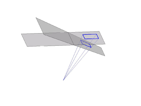
Figure 5: $\Gamma_{\boldsymbol{\mathit{u}},\boldsymbol{\mathit{v}}}$ can be understood as the projection through the origin from one plane onto the other.

Lemma 5.2.9 (Jacobian of $\Psi$).

$$\left|\frac{\partial\Psi(\boldsymbol{\tilde{\alpha}})}{\partial\boldsymbol{\tilde{\alpha}}}\right|=\mbox{{\bf det}}\left(\boldsymbol{\mathit{A}}^{-1}\boldsymbol{\tilde{\mathit{A}}}\right)\frac{\left\|\mathbf{1}\right\|}{\left<\boldsymbol{\mathit{A}}^{-1}\boldsymbol{\tilde{\mathit{A}}}\boldsymbol{\tilde{\alpha}}|\mathbf{1}\right>^{d}\left\|\left(\boldsymbol{\tilde{\mathit{A}}}^{-1}\boldsymbol{\mathit{A}}\right)^{T}\mathbf{1}\right\|}.$$

Proof.

Let $\boldsymbol{\alpha}=\Psi(\boldsymbol{\tilde{\alpha}})$ and let $\boldsymbol{\alpha}^{\prime}=\boldsymbol{\mathit{A}}^{-1}\boldsymbol{\tilde{\mathit{A}}}\boldsymbol{\tilde{\alpha}}$. As $\left<\boldsymbol{\tilde{\alpha}}|\mathbf{1}\right>=1$, we have

$$\left<\boldsymbol{\alpha}^{\prime}|\left(\boldsymbol{\tilde{\mathit{A}}}^{-1}\boldsymbol{\mathit{A}}\right)^{T}\mathbf{1}\right>=1.$$

So, $\boldsymbol{\alpha}=\Gamma_{\boldsymbol{\mathit{u}},\boldsymbol{\mathit{v}}}(\boldsymbol{\alpha}^{\prime})$, where $\boldsymbol{\mathit{u}}=\left(\boldsymbol{\tilde{\mathit{A}}}^{-1}\boldsymbol{\mathit{A}}\right)^{T}\mathbf{1}$ and $\boldsymbol{\mathit{v}}=\mathbf{1}$. By Lemma 5.2.11,

$$\left|\frac{\partial\boldsymbol{\alpha}}{\partial\boldsymbol{\tilde{\alpha}}}\right|=\left|\frac{\partial\boldsymbol{\alpha}}{\partial\boldsymbol{\alpha}^{\prime}}\right|\left|\frac{\partial\boldsymbol{\alpha}^{\prime}}{\partial\boldsymbol{\tilde{\alpha}}}\right| =\mbox{{\bf det}}\left(\frac{\partial\Gamma_{\boldsymbol{\mathit{u}},\boldsymbol{\mathit{v}}}(\boldsymbol{\alpha}^{\prime})}{\partial\boldsymbol{\alpha}^{\prime}}\right)\mbox{{\bf det}}\left(\boldsymbol{\mathit{A}}^{-1}\boldsymbol{\tilde{\mathit{A}}}\right)$$

$$=\mbox{{\bf det}}\left(\boldsymbol{\mathit{A}}^{-1}\boldsymbol{\tilde{\mathit{A}}}\right)\frac{\left\|\mathbf{1}\right\|}{\left<\boldsymbol{\mathit{A}}^{-1}\boldsymbol{\tilde{\mathit{A}}}\boldsymbol{\tilde{\alpha}}|\mathbf{1}\right>^{d}\left\|\left(\boldsymbol{\tilde{\mathit{A}}}^{-1}\boldsymbol{\mathit{A}}\right)^{T}\mathbf{1}\right\|}.$$

Lemma 5.2.10 (Bound on Jacobian of $\Psi$).

Under the conditions of Lemma 5.2.5,

$$\left|\frac{\partial\Psi(\boldsymbol{\tilde{\alpha}})}{\partial\boldsymbol{\tilde{\alpha}}}\right|\leq\frac{(1+\epsilon)^{d}}{(1-\epsilon\sqrt{d})^{d}(1-\epsilon)}.$$

for all $\boldsymbol{\tilde{\alpha}}\in A_{0}$.

Proof.

The condition $\left\|I-\boldsymbol{\mathit{A}}^{-1}\boldsymbol{\tilde{\mathit{A}}}\right\|\leq\epsilon$ implies $\left\|\boldsymbol{\mathit{A}}^{-1}\boldsymbol{\tilde{\mathit{A}}}\right\|\leq 1+\epsilon$, so Proposition 2.2.4 (e) implies

$$\mbox{{\bf det}}\left(\boldsymbol{\mathit{A}}^{-1}\boldsymbol{\tilde{\mathit{A}}}\right)\leq(1+\epsilon)^{d}.$$

Observing that $\left\|\mathbf{1}\right\|=\sqrt{d}$, and $\left\|I-(\boldsymbol{\tilde{\mathit{A}}}^{-1}\boldsymbol{\mathit{A}})^{T}\right\|=\left\|I-(\boldsymbol{\tilde{\mathit{A}}}^{-1}\boldsymbol{\mathit{A}})\right\|$, we compute

$$\left\|(\boldsymbol{\tilde{\mathit{A}}}^{-1}\boldsymbol{\mathit{A}})^{T}\mathbf{1}\right\|\geq\left\|\mathbf{1}\right\|-\left\|\mathbf{1}-(\boldsymbol{\tilde{\mathit{A}}}^{-1}\boldsymbol{\mathit{A}})^{T}\mathbf{1}\right\|\geq\sqrt{d}-\left\|I-(\boldsymbol{\tilde{\mathit{A}}}^{-1}\boldsymbol{\mathit{A}})^{T}\right\|\left\|\mathbf{1}\right\|\geq\sqrt{d}-\epsilon\sqrt{d}.$$

So,

$$\frac{\left\|\mathbf{1}\right\|}{\left\|\left(\boldsymbol{\tilde{\mathit{A}}}^{-1}\boldsymbol{\mathit{A}}\right)^{T}\mathbf{1}\right\|}\leq\frac{1}{1-\epsilon}.$$

Finally, as $\left<\boldsymbol{\tilde{\alpha}}|\mathbf{1}\right>=1$ and $\left\|\boldsymbol{\tilde{\alpha}}\right\|\leq 1$, we have

$$\left<\boldsymbol{\mathit{A}}^{-1}\boldsymbol{\tilde{\mathit{A}}}\boldsymbol{\tilde{\alpha}}|\mathbf{1}\right> =\left<\boldsymbol{\tilde{\alpha}}|\mathbf{1}\right>+\left<\boldsymbol{\mathit{A}}^{-1}\boldsymbol{\tilde{\mathit{A}}}\boldsymbol{\tilde{\alpha}}-\boldsymbol{\tilde{\alpha}}|\mathbf{1}\right>$$

$$=1+\left<(\boldsymbol{\mathit{A}}^{-1}\boldsymbol{\tilde{\mathit{A}}}-I)\boldsymbol{\tilde{\alpha}}|\mathbf{1}\right>$$

$$\geq 1-\left\|\boldsymbol{\mathit{A}}^{-1}\boldsymbol{\tilde{\mathit{A}}}-I\right\|\left\|\boldsymbol{\tilde{\alpha}}\right\|\left\|\mathbf{1}\right\|$$

$$\geq 1-\epsilon\sqrt{d}.$$

Applying Lemma 5.2.9, we have

$$\left|\frac{\partial\Psi(\boldsymbol{\tilde{\alpha}})}{\partial\boldsymbol{\tilde{\alpha}}}\right|=\mbox{{\bf det}}\left(\boldsymbol{\mathit{A}}^{-1}\boldsymbol{\tilde{\mathit{A}}}\right)\frac{\left\|\mathbf{1}\right\|}{\left<\boldsymbol{\mathit{A}}^{-1}\boldsymbol{\tilde{\mathit{A}}}\boldsymbol{\alpha}|\mathbf{1}\right>^{d}\left\|\left(\boldsymbol{\tilde{\mathit{A}}}^{-1}\boldsymbol{\mathit{A}}\right)^{T}\mathbf{1}\right\|}\leq\frac{(1+\epsilon)^{d}}{(1-\epsilon\sqrt{d})^{d}(1-\epsilon)}.$$

Lemma 5.2.11 (Jacobian of $\Gamma_{\boldsymbol{\mathit{u}},\boldsymbol{\mathit{v}}}$).

$$\left|\mbox{{\bf det}}\left(\frac{\partial\Gamma_{\boldsymbol{\mathit{u}},\boldsymbol{\mathit{v}}}(\boldsymbol{\mathit{x}})}{\partial\boldsymbol{\mathit{x}}}\right)\right|=\frac{\left\|\boldsymbol{\mathit{v}}\right\|}{\left<\boldsymbol{\mathit{x}}|\boldsymbol{\mathit{v}}\right>^{d}\left\|\boldsymbol{\mathit{u}}\right\|}.$$

Proof.

Consider dividing ${\rm I\kern-2.0ptR}^{d}$ into $\textbf{Span}\left(\boldsymbol{\mathit{u}},\boldsymbol{\mathit{v}}\right)$ and the space orthogonal to $\textbf{Span}\left(\boldsymbol{\mathit{u}},\boldsymbol{\mathit{v}}\right)$. In the $(d-2)$-dimensional orthogonal space, $\Gamma_{\boldsymbol{\mathit{u}},\boldsymbol{\mathit{v}}}$ acts as a multiplication by $1/\left<\boldsymbol{\mathit{x}}|\boldsymbol{\mathit{v}}\right>$. On the other hand, the Jacobian of the restriction of $\Gamma_{\boldsymbol{\mathit{u}},\boldsymbol{\mathit{v}}}$ to $\textbf{Span}\left(\boldsymbol{\mathit{u}},\boldsymbol{\mathit{v}}\right)$ is computed by Lemma 5.2.12 to be

$$\frac{\left\|\boldsymbol{\mathit{v}}\right\|}{\left<\boldsymbol{\mathit{x}}|\boldsymbol{\mathit{v}}\right>^{2}\left\|\boldsymbol{\mathit{u}}\right\|}.$$

So,

$$\left|\mbox{{\bf det}}\left(\frac{\partial\Gamma_{\boldsymbol{\mathit{u}},\boldsymbol{\mathit{v}}}(\boldsymbol{\mathit{x}})}{\partial\boldsymbol{\mathit{x}}}\right)\right|=\left(\frac{1}{\left<\boldsymbol{\mathit{x}}|\boldsymbol{\mathit{v}}\right>}\right)^{d-2}\frac{\left\|\boldsymbol{\mathit{v}}\right\|}{\left<\boldsymbol{\mathit{x}}|\boldsymbol{\mathit{v}}\right>^{2}\left\|\boldsymbol{\mathit{u}}\right\|}=\frac{\left\|\boldsymbol{\mathit{v}}\right\|}{\left<\boldsymbol{\mathit{x}}|\boldsymbol{\mathit{v}}\right>^{d}\left\|\boldsymbol{\mathit{u}}\right\|}.$$

Lemma 5.2.12 (Jacobian of $\Gamma_{\boldsymbol{\mathit{u}},\boldsymbol{\mathit{v}}}$ in 2D).

Let $\boldsymbol{\mathit{u}}$ and $\boldsymbol{\mathit{v}}$ be vectors in ${\rm I\kern-2.0ptR}^{2}$ and let $\Gamma_{\boldsymbol{\mathit{u}},\boldsymbol{\mathit{v}}}(\boldsymbol{\mathit{x}})$ be the map from $\left\{\boldsymbol{\mathit{x}}:\left<\boldsymbol{\mathit{x}}|\boldsymbol{\mathit{u}}\right>=1\right\}$ to $\left\{\boldsymbol{\mathit{x}}:\left<\boldsymbol{\mathit{x}}|\boldsymbol{\mathit{v}}\right>=1\right\}$ by

$$\Gamma_{\boldsymbol{\mathit{u}},\boldsymbol{\mathit{v}}}(\boldsymbol{\mathit{x}})=\frac{\boldsymbol{\mathit{x}}}{\left<\boldsymbol{\mathit{x}}|\boldsymbol{\mathit{v}}\right>}.$$

Then,

$$\left|\mbox{{\bf det}}\left(\frac{\partial\Gamma_{\boldsymbol{\mathit{u}},\boldsymbol{\mathit{v}}}(\boldsymbol{\mathit{x}})}{\partial\boldsymbol{\mathit{x}}}\right)\right|=\frac{\left\|\boldsymbol{\mathit{v}}\right\|}{\left<\boldsymbol{\mathit{x}}|\boldsymbol{\mathit{v}}\right>^{2}\left\|\boldsymbol{\mathit{u}}\right\|}.$$

Proof.

Let $\boldsymbol{\mathit{R}}=\left(\begin{array}[]{rr}0&-1\\ 1&0\end{array}\right)$, the $90^{o}$ rotation counter-clockwise. Let

$$\boldsymbol{\mathit{u}}^{\bot}=\boldsymbol{\mathit{R}}\boldsymbol{\mathit{u}}/\left\|\boldsymbol{\mathit{u}}\right\|\qquad\text{ and }\qquad\boldsymbol{\mathit{v}}^{\bot}=\boldsymbol{\mathit{R}}\boldsymbol{\mathit{v}}/\left\|\boldsymbol{\mathit{v}}\right\|.$$

Express the $\boldsymbol{\mathit{x}}$ such that $\left<\boldsymbol{\mathit{x}}|\boldsymbol{\mathit{u}}\right>=1$, as $\boldsymbol{\mathit{x}}=\boldsymbol{\mathit{u}}/\left\|\boldsymbol{\mathit{u}}\right\|^{2}+x\boldsymbol{\mathit{u}}^{\bot}$. Similarly, parameterize the line $\left\{\boldsymbol{\mathit{x}}:\left<\boldsymbol{\mathit{x}}|\boldsymbol{\mathit{v}}\right>=1\right\}$ by $\boldsymbol{\mathit{v}}/\left\|\boldsymbol{\mathit{v}}\right\|^{2}+y\boldsymbol{\mathit{v}}^{\bot}$. Then, we have

$$\Gamma_{\boldsymbol{\mathit{u}},\boldsymbol{\mathit{v}}}\left(u/\left\|\boldsymbol{\mathit{u}}\right\|^{2}+x\boldsymbol{\mathit{u}}^{\bot}\right)=\boldsymbol{\mathit{v}}/\left\|\boldsymbol{\mathit{v}}\right\|^{2}+y\boldsymbol{\mathit{v}}^{\bot},$$

where

$$y=\frac{\left<u/\left\|\boldsymbol{\mathit{u}}\right\|^{2}+x\boldsymbol{\mathit{u}}^{\bot}|\boldsymbol{\mathit{v}}^{\bot}\right>}{\left<u/\left\|\boldsymbol{\mathit{u}}\right\|^{2}+x\boldsymbol{\mathit{u}}^{\bot}|\boldsymbol{\mathit{v}}\right>}=\frac{\left<u/\left\|\boldsymbol{\mathit{u}}\right\|^{2}+x\boldsymbol{\mathit{u}}^{\bot}|\boldsymbol{\mathit{v}}^{\bot}\right>}{\left<\boldsymbol{\mathit{x}}|\boldsymbol{\mathit{v}}\right>}.$$

So,

$$\left|\mbox{{\bf det}}\left(\frac{\partial\Gamma_{\boldsymbol{\mathit{u}},\boldsymbol{\mathit{v}}}(\boldsymbol{\mathit{x}})}{\partial\boldsymbol{\mathit{x}}}\right)\right| =\left|\mbox{{\bf det}}\left(\frac{\partial y}{\partial x}\right)\right|$$

$$=\left|\frac{\left<\boldsymbol{\mathit{u}}^{\bot}\Big{|}\boldsymbol{\mathit{v}}^{\bot}\right>\left<\frac{\boldsymbol{\mathit{u}}}{\left\|\boldsymbol{\mathit{u}}\right\|^{2}}+x\boldsymbol{\mathit{u}}^{\bot}\Big{|}\boldsymbol{\mathit{v}}\right>-\left<\boldsymbol{\mathit{u}}^{\bot}\Big{|}\boldsymbol{\mathit{v}}\right>\left<\frac{\boldsymbol{\mathit{u}}}{\left\|\boldsymbol{\mathit{u}}\right\|^{2}}+x\boldsymbol{\mathit{u}}^{\bot}\Big{|}\boldsymbol{\mathit{v}}^{\bot}\right>}{\left<\boldsymbol{\mathit{x}}|\boldsymbol{\mathit{v}}\right>^{2}}\right|$$

$$=\left|\frac{\left<\boldsymbol{\mathit{u}}^{\bot}\Big{|}\boldsymbol{\mathit{v}}^{\bot}\right>\left<\frac{\boldsymbol{\mathit{u}}}{\left\|\boldsymbol{\mathit{u}}\right\|^{2}}\Big{|}\boldsymbol{\mathit{v}}\right>-\left<\boldsymbol{\mathit{u}}^{\bot}\Big{|}\boldsymbol{\mathit{v}}\right>\left<\frac{\boldsymbol{\mathit{u}}}{\left\|\boldsymbol{\mathit{u}}\right\|^{2}}\Big{|}\boldsymbol{\mathit{v}}^{\bot}\right>}{\left<\boldsymbol{\mathit{x}}|\boldsymbol{\mathit{v}}\right>^{2}}\right|$$

$$=\left|\frac{\left\|\boldsymbol{\mathit{v}}\right\|\left(\left<\boldsymbol{\mathit{u}}^{\bot}\Big{|}\boldsymbol{\mathit{v}}^{\bot}\right>\left<\frac{u}{\left\|\boldsymbol{\mathit{u}}\right\|}\Big{|}\frac{v}{\left\|\boldsymbol{\mathit{v}}\right\|}\right>-\left<\boldsymbol{\mathit{u}}^{\bot}\Big{|}\frac{v}{\left\|\boldsymbol{\mathit{v}}\right\|}\right>\left<\frac{u}{\left\|\boldsymbol{\mathit{u}}\right\|}\Big{|}\boldsymbol{\mathit{v}}^{\bot}\right>\right)}{\left\|\boldsymbol{\mathit{u}}\right\|\left<\boldsymbol{\mathit{x}}|\boldsymbol{\mathit{v}}\right>^{2}}\right|$$

$$=\left|\frac{\left\|\boldsymbol{\mathit{v}}\right\|\left(\left<\frac{u}{\left\|\boldsymbol{\mathit{u}}\right\|}\Big{|}\frac{v}{\left\|\boldsymbol{\mathit{v}}\right\|}\right>^{2}+\left<\boldsymbol{\mathit{u}}^{\bot}\Big{|}\frac{v}{\left\|\boldsymbol{\mathit{v}}\right\|}\right>^{2}\right)}{\left\|\boldsymbol{\mathit{u}}\right\|\left<\boldsymbol{\mathit{x}}|\boldsymbol{\mathit{v}}\right>^{2}}\right|,\text{ as $\boldsymbol{\mathit{R}}$ is orthogonal and $\boldsymbol{\mathit{R}}^{2}=-1$,}$$

$$=\frac{\left\|\boldsymbol{\mathit{v}}\right\|}{\left\|\boldsymbol{\mathit{u}}\right\|\left<\boldsymbol{\mathit{x}}|\boldsymbol{\mathit{v}}\right>^{2}},\text{ as $\frac{\boldsymbol{\mathit{u}}}{\left\|\boldsymbol{\mathit{u}}\right\|},\boldsymbol{\mathit{u}}^{\bot}$ is a basis.}$$

5.3 Bounding the shadow of $LP^{+}$

The main obstacle to proving a bound on the size of the shadow of $LP^{+}$ is that the vectors $\boldsymbol{\mathit{a}}^{+}_{i}/y^{+}_{i}$ are not Gaussian random vectors. To resolve this problem, we will show that, in almost every sufficiently small region, we can construct a family of Gaussian random vectors with distributions similar to the vectors $\boldsymbol{\mathit{a}}^{+}_{i}/y^{+}_{i}$. We will then bound the expected size of the shadow of the vectors $\boldsymbol{\mathit{a}}^{+}_{i}/y^{+}_{i}$ by a small multiple of the expected size of the shadow of these Gaussian vectors. These regions are defined by splitting the original perturbation into two, and letting the first perturbation define the region.

As in the analysis of $LP^{\prime}$, a secondary obstacle is the correlation of $\kappa$ and $M$ with $\boldsymbol{\mathit{A}}$ and $\boldsymbol{\mathit{y}}$. We again overcome this obstacle by considering the sum of the expected sizes of the shadows when $\kappa$ and $M$ are fixed to each of their likely values, and use the notation

$$\mathcal{T}^{+}_{\boldsymbol{\mathit{z}}}(\boldsymbol{\mathit{A}},\boldsymbol{\mathit{y}},\kappa,M)\stackrel{{\scriptstyle\mathrm{def}}}{{=}}\begin{cases}\left|\mbox{{\bf Shadow}}_{(0,\boldsymbol{\mathit{z}}),\boldsymbol{\mathit{z}}^{+}}\left(\boldsymbol{\mathit{a}}^{+}_{1}/y^{+}_{1},\ldots,\boldsymbol{\mathit{a}}^{+}_{n}/y^{+}_{n}\right)\right|,&\text{if $\sqrt{d}M/4\kappa\geq 1$}\\ 0&\text{otherwise},\end{cases}$$

where

$$\boldsymbol{\mathit{a}}^{+}_{i} =\left((y^{\prime}_{i}-y_{i})/2,\boldsymbol{\mathit{a}}_{i}\right),$$

$$y^{+}_{i} =(y^{\prime}_{i}+y_{i})/2,\text{ and}$$

$$y_{i}^{\prime} =\begin{cases}M&\text{if $i\in I$}\\ \sqrt{d}M^{2}/4\kappa&\text{otherwise.}\end{cases}$$

By Lemma 3.3.5 and Proposition 3.3.2, we then have

$$\mathcal{S}^{+}_{\boldsymbol{\mathit{z}}}(\boldsymbol{\mathit{A}},\boldsymbol{\mathit{y}},\mathcal{I})=\mathcal{T}^{+}_{\boldsymbol{\mathit{z}}}\left(\boldsymbol{\mathit{A}},\boldsymbol{\mathit{y}},2^{\left\lfloor\lg\mbox{\bf s}_{\textbf{min}}\left(\boldsymbol{\mathit{A}}_{\mathcal{I}(\boldsymbol{\mathit{A}})}\right)\right\rfloor},2^{\left\lceil\lg(\max_{i}\left\|(y_{i},\boldsymbol{\mathit{a}}_{i})\right\|)\right\rceil+2}\right).$$

Lemma 5.3.1 (LP+).

Let $d\geq 3$ and $n\geq d+1$. Let $\bar{\boldsymbol{\mathit{A}}}=[\bar{\boldsymbol{\mathit{a}}}_{1},\ldots,\bar{\boldsymbol{\mathit{a}}}_{n}]\in{\rm I\kern-2.0ptR}^{n\times d}$, $\bar{\boldsymbol{\mathit{y}}}\in{\rm I\kern-2.0ptR}^{n}$ and $\boldsymbol{\mathit{z}}\in{\rm I\kern-2.0ptR}^{d}$, satisfy $\max_{i}\left\|(\bar{y}_{i},\bar{\boldsymbol{\mathit{a}}}_{i})\right\|\in(1/2,1]$. For any $\sigma>0$, let $\boldsymbol{\mathit{A}}$ be a Gaussian random matrix centered at $\bar{\boldsymbol{\mathit{A}}}$ of standard deviation $\sigma$, and let $\boldsymbol{\mathit{y}}$ by a Gaussian random vector centered at $\bar{\boldsymbol{\mathit{y}}}$ of standard deviation $\sigma$. Let $\mathcal{I}$ be a set of $3nd\ln n$ randomly chosen $d$-subsets of $[n]$. Then,

$$\operatorname{\textbf{E}}\displaylimits_{\boldsymbol{\mathit{A}},\boldsymbol{\mathit{y}},\mathcal{I}}\left[\mathcal{S}^{+}(\boldsymbol{\mathit{A}},\boldsymbol{\mathit{y}},\mathcal{I})\right]\leq 49\lg(nd/\min(\sigma,1))\mathcal{D}\left(d,n,\frac{\min(1,\sigma^{5})}{2^{23}(d+1)^{11/2}n^{14}(\ln n)^{5/2}}\right)+n.$$

where $\mathcal{D}(d,n,\sigma)$ is as given in Theorem 4.0.1.

Proof.

For $\rho_{0}$ and $\rho_{1}$ defined below, we let $\boldsymbol{\mathit{G}}$ and $\boldsymbol{\tilde{\mathit{G}}}$ be Gaussian random matrices centered at the origin of standard deviations $\rho_{0}$ and $\rho_{1}$, respectively. We then let $\boldsymbol{\tilde{\mathit{A}}}=\bar{\boldsymbol{\mathit{A}}}+\boldsymbol{\mathit{G}}$ and $\boldsymbol{\mathit{A}}=\boldsymbol{\tilde{\mathit{A}}}+\boldsymbol{\tilde{\mathit{G}}}$. We similarly let $\boldsymbol{\mathit{h}}$ and $\tilde{\boldsymbol{\mathit{h}}}$ be Gaussian random vectors centered at the origin of standard deviations $\rho_{0}$ and $\rho_{1}$, respectively, and let $\tilde{\boldsymbol{\mathit{y}}}=\boldsymbol{\mathit{y}}^{\prime}+\boldsymbol{\mathit{h}}$ and $\boldsymbol{\mathit{y}}=\tilde{\boldsymbol{\mathit{y}}}+\tilde{\boldsymbol{\mathit{h}}}$. If

$$\sigma\leq\frac{3\sqrt{1/4}}{\sqrt{2e}n(60n(d+1)^{3/2}(\ln n)^{3/2})},$$

we set $\rho_{1}=\sigma$. Otherwise, we set $\rho_{1}$ so that

$$\rho_{1}=\frac{3\sqrt{1/4+d(\sigma^{2}-\rho_{1}^{2})}}{\sqrt{2e}n(60n(d+1)^{3/2}(\ln n)^{3/2})},$$

and set $\rho_{0}^{2}=\sigma^{2}-\rho_{1}^{2}$. We note that

$$\rho_{1}=\min\left(\sigma,\frac{3\sqrt{1/4+d\rho_{0}^{2}}}{\sqrt{2e}n(60n(d+1)^{3/2}(\ln n)^{3/2})}\right).$$

As in the proof of Lemma 5.2.1, we define the set of likely values for $M$:

$$\mathcal{M}=\Bigg{\{}2^{\left\lceil\lg x\right\rceil+2}:\left(\max_{i}\left\|(\tilde{y}_{i},\tilde{\boldsymbol{\mathit{a}}}_{i})\right\|\right)\left(1-\frac{9\sqrt{(d+1)\ln n}}{(60n(d+1)^{3/2}(\ln n)^{3/2})}\right)\leq x\\ \leq\left(\max_{i}\left\|(\tilde{y}_{i},\tilde{\boldsymbol{\mathit{a}}}_{i})\right\|\right)\left(1+\frac{9\sqrt{(d+1)\ln n}}{(60n(d+1)^{3/2}(\ln n)^{3/2})}\right)\Bigg{\}}.$$

Observed that $\left|\mathcal{M}\right|\leq 2$.

As in the proof of Lemma 5.2.1, we define random variables:

$$W =\left[\max_{i}\left\|(\tilde{y}_{i},\tilde{\boldsymbol{\mathit{a}}}_{i})\right\|\leq 1+3\sqrt{(d+1)\ln n}\rho_{0}\right],$$

$$X =\left[\max_{i}\left\|(\tilde{y}_{i},\tilde{\boldsymbol{\mathit{a}}}_{i})\right\|\geq\frac{\sqrt{1/4+d\rho_{0}^{2}}}{\sqrt{2e}n}\right],$$

$$Y =\left[2^{\left\lfloor\lg\mbox{\bf s}_{\textbf{min}}\left(\boldsymbol{\mathit{A}}_{\mathcal{I}(\boldsymbol{\mathit{A}})}\right)\right\rfloor}\in\mathcal{K}\right],\text{ and}$$

$$Z =\left[2^{\left\lceil\lg\max_{i}\left\|(y_{i},\boldsymbol{\mathit{a}}_{i})\right\|\right\rceil+2}\in\mathcal{M}\right].$$

In order to apply the shadow bound proved below in Lemma 5.3.2, we need

$$M\geq 3\max_{i}\left\|(\tilde{y}_{i},\tilde{\boldsymbol{\mathit{a}}}_{i})\right\|,$$

and

$$M\geq(60n(d+1)^{3/2}(\ln n)^{3/2})\rho_{1}.$$

From the definition of $\mathcal{M}$ and the inequality $1-9\sqrt{(d+1)\ln n}/(60n(d+1)^{3/2}(\ln n)^{3/2})\geq 3/4$, the first of these inequalities holds if $Z$ is true. Given that $Z$ is true, the second inequality holds if $X$ is also true.

From Corollary 5.1.3, we know

$$\operatorname{\textbf{Pr}}\displaylimits_{\boldsymbol{\mathit{A}},\mathcal{I}}\left[\mathrm{not}(Y)\right]\leq\operatorname{\textbf{Pr}}\displaylimits_{\boldsymbol{\mathit{A}},\mathcal{I}}\left[2^{\left\lfloor\lg\mbox{\bf s}_{\textbf{min}}\left(\boldsymbol{\mathit{A}}_{\mathcal{I}(\boldsymbol{\mathit{A}})}\right)\right\rfloor}\not\in\mathcal{K}\right]\leq 0.42\binom{n}{d}^{-1}\leq 0.42n\binom{n}{d+1}^{-1}.$$ (55)

From Corollary 2.4.6 we have

$$\operatorname{\textbf{Pr}}\displaylimits_{\boldsymbol{\tilde{\mathit{A}}},\tilde{\boldsymbol{\mathit{y}}}}\left[\mathrm{not}(W)\right]\leq n^{-2.9(d+1)+1}\leq 0.0015\binom{n}{d+1}^{-1}.$$ (56)

From Proposition 2.4.9, we know

$$\operatorname{\textbf{Pr}}\displaylimits\left[\mathrm{not}(X)\right]=\operatorname{\textbf{Pr}}\displaylimits\left[\max_{i}\left\|(\tilde{y}_{i},\tilde{\boldsymbol{\mathit{a}}}_{i})\right\|<\frac{\sqrt{1/4+d\rho_{0}^{2}}}{\sqrt{2e}n}\right]<n^{-(d+1)}\leq\frac{1}{24}\binom{n}{d+1}^{-1}.$$ (57)

To bound the probability that $Z$ fails, we note that

$$\max_{i}\left\|(\tilde{y}_{i},\tilde{\boldsymbol{\mathit{a}}}_{i})\right\|\geq\frac{\sqrt{1/4+d\rho_{0}^{2}}}{\sqrt{2e}n}$$

and

$$\max_{i}\left\|(y_{i}-\tilde{y}_{i},\boldsymbol{\mathit{a}}_{i}-\tilde{\boldsymbol{\mathit{a}}}_{i})\right\|\leq\rho_{1}3\sqrt{(d+1)\ln n},$$

imply $Z$ is true. Hence, by Corollary 2.4.6 and (57),

$$\operatorname{\textbf{Pr}}\displaylimits\left[\mathrm{not(Z)}\right]\leq n^{-2.9(d+1)+1}+n^{-(d+1)}\leq.044\binom{n}{d+1}^{-1}.$$ (58)

As in the proof of Lemma 5.2.1, we now expand

$$\operatorname{\textbf{E}}\displaylimits_{\mathcal{I},A,\boldsymbol{\mathit{y}}}\left[\mathcal{S}^{+}(\boldsymbol{\mathit{A}},\boldsymbol{\mathit{y}},\mathcal{I})\right]=\operatorname{\textbf{E}}\displaylimits_{\mathcal{I},A,\boldsymbol{\mathit{y}}}\left[\mathcal{S}^{+}(\boldsymbol{\mathit{A}},\boldsymbol{\mathit{y}},\mathcal{I})WXYZ\right]+\operatorname{\textbf{E}}\displaylimits_{\mathcal{I},A,\boldsymbol{\mathit{y}}}\left[\mathcal{S}^{+}(\boldsymbol{\mathit{A}},\boldsymbol{\mathit{y}},\mathcal{I})(1-WXYZ)\right].$$ (59)

To bound the second term by $n$, we apply (56) , (57) , (55) and (58) to show

$$\operatorname{\textbf{Pr}}\displaylimits_{\boldsymbol{\mathit{A}},\mathcal{I}}\left[\mathrm{not}(W)\text{ or }\mathrm{not}(X)\text{ or }\mathrm{not}(Y)\text{ or }\mathrm{not}(Z)\right]\leq n\binom{n}{d+1}^{-1},$$

and then combine this inequality with Proposition 5.0.2.

To bound the first term of (59), we note

$$\operatorname{\textbf{E}}\displaylimits_{\mathcal{I},A,\boldsymbol{\mathit{y}}}\left[\mathcal{S}^{+}(\boldsymbol{\mathit{A}},\boldsymbol{\mathit{y}},\mathcal{I})WXYZ\right]$$

$$\leq\operatorname{\textbf{E}}\displaylimits_{\mathcal{I},\boldsymbol{\tilde{\mathit{A}}},\tilde{\boldsymbol{\mathit{y}}}}\left[WX\sum_{\kappa\in\mathcal{K},M\in\mathcal{M}}\operatorname{\textbf{E}}\displaylimits_{\boldsymbol{\tilde{\mathit{G}}},\tilde{\boldsymbol{\mathit{h}}}}\left[\mathcal{T}^{+}\left(\boldsymbol{\mathit{A}},\boldsymbol{\mathit{y}},\kappa,M\right)XZ\right]\right]$$

$$\leq\operatorname{\textbf{E}}\displaylimits_{\mathcal{I},\boldsymbol{\tilde{\mathit{A}}},\tilde{\boldsymbol{\mathit{y}}}}\left[WX\sum_{\kappa\in\mathcal{K},M\in\mathcal{M}}\operatorname{\textbf{E}}\displaylimits_{\boldsymbol{\tilde{\mathit{G}}},\tilde{\boldsymbol{\mathit{h}}}}\left[\mathcal{T}^{+}\left(\boldsymbol{\mathit{A}},\boldsymbol{\mathit{y}},\kappa,M\right)\Big{|}XZ\right]\right]$$

$$\leq\operatorname{\textbf{E}}\displaylimits_{\mathcal{I},\boldsymbol{\tilde{\mathit{A}}},\tilde{\boldsymbol{\mathit{y}}}}\left[WX\sum_{\kappa\in\mathcal{K},M\in\mathcal{M}}e\mathcal{D}\left(d,n,\frac{\rho_{1}\min_{i}y^{\prime}_{i}}{3(\max_{i}y^{\prime}_{i})^{2}}\right)+1,\right]\text{ by Lemma~{}\ref{lem:lp+2} }$$ (60)

$$\leq\operatorname{\textbf{E}}\displaylimits_{\mathcal{I},\boldsymbol{\tilde{\mathit{A}}},\tilde{\boldsymbol{\mathit{y}}}}\left[WX\sum_{\kappa\in\mathcal{K},M\in\mathcal{M}}e\mathcal{D}\left(d,n,\frac{\sigma M}{3(M^{2}/4\kappa)^{2}}\right)+1\right]$$

$$\leq\operatorname{\textbf{E}}\displaylimits_{\mathcal{I},\boldsymbol{\tilde{\mathit{A}}},\tilde{\boldsymbol{\mathit{y}}}}\left[WX\left|\mathcal{K}\right|\left|M\right|e\mathcal{D}\left(d,n,\frac{16\sigma\min(\mathcal{K})^{2}}{3\max(\mathcal{M})^{3}}\right)+1\right].$$ (61)

As $\min(\mathcal{K})\geq\kappa_{0}/2$ and $W$ implies $\max(\mathcal{M})\leq 9\left(1+3\sqrt{(d+1)\ln n}\sigma\right)$,

$$\frac{16\sigma\min(\mathcal{K})^{2}}{3\max(\mathcal{M})^{3}} \geq\frac{16\sigma^{3}\min(1,\sigma)^{2}}{3\cdot 4\left(9(1+3\sqrt{(d+1)\ln n}\sigma\right)^{3}\left(12d^{2}n^{7}\sqrt{\ln n}\right)^{2}}$$

$$\geq\frac{16\min(1,\sigma^{5})}{3\cdot 4\left(9(1+3\sqrt{(d+1)\ln n}\right)^{3}\left(12d^{2}n^{7}\sqrt{\ln n}\right)^{2}}$$

$$\geq\frac{\min(1,\sigma^{5})}{2^{23}(d+1)^{11/2}n^{14}(\ln n)^{5/2}}.$$

Applying this inequality, Proposition 5.1.4, and the fact that $X$ implies $\left|\mathcal{M}\right|\leq 2$, we obtain

$$\eqref{eqn:lp+a}\leq 49\lg(nd/\min(\sigma,1))\mathcal{D}\left(d,n,\frac{\min(1,\sigma^{5})}{2^{23}(d+1)^{11/2}n^{14}(\ln n)^{5/2}}\right).$$

Lemma 5.3.2 ($LP^{+}$ Shadow, part 2).

Let $d\geq 3$ and $n\geq d+1$. Let $\boldsymbol{\mathit{y}}$ be a Gaussian random vector of standard deviation $\rho_{1}$ centered at a point $\tilde{\boldsymbol{\mathit{y}}}$, and let $\boldsymbol{\mathit{a}}_{1},\ldots,\boldsymbol{\mathit{a}}_{n}$ be Gaussian random vectors in ${\rm I\kern-2.0ptR}^{d}$ of standard deviation $\rho_{1}$ centered at $\tilde{\boldsymbol{\mathit{a}}}_{1},\ldots,\tilde{\boldsymbol{\mathit{a}}}_{n}$ respectively. Under the conditions

$$y_{i}^{\prime} >3(\left\|\tilde{y}_{i},\tilde{\boldsymbol{\mathit{a}}}_{i}\right\|),\forall i,\text{ and}$$ (62)

$$y_{i}^{\prime} >60n(d+1)^{3/2}(\ln n)^{3/2}\rho_{1},\forall i.$$ (63)

Let

$$\boldsymbol{\mathit{a}}^{+}_{i} =\left((y^{\prime}_{i}-y_{i})/2,\boldsymbol{\mathit{a}}_{i}\right),\text{and}$$

$$y^{+}_{i} =(y^{\prime}_{i}+y_{i})/2.$$

Then,

$$\operatorname{\textbf{E}}\displaylimits_{(y_{1},\boldsymbol{\mathit{a}}_{1}),\ldots,(y_{n},\boldsymbol{\mathit{a}}_{n})}\left[\left|\mbox{{\bf Shadow}}_{(0,\boldsymbol{\mathit{z}}),\boldsymbol{\mathit{z}}^{+}}\left(\boldsymbol{\mathit{a}}^{+}_{1}/y^{+}_{1},\ldots,\boldsymbol{\mathit{a}}^{+}_{n}/y^{+}_{n}\right)\right|\right]\leq e\mathcal{D}\left(d,n,\frac{\rho_{1}\min_{i}y^{\prime}_{i}}{3(\max_{i}y^{\prime}_{i})^{2}}\right)+1.$$

Proof.

We use the notation

$$(p_{i,0}(\tilde{h}_{i}),\boldsymbol{\mathit{p}}_{i}(\tilde{h}_{i},\tilde{\boldsymbol{\mathit{g}}}_{i}))=\boldsymbol{\mathit{a}}^{+}_{i}/y^{+}_{i}=\left(\frac{y_{i}^{\prime}-\tilde{y}_{i}-\tilde{h}_{i}}{y_{i}^{\prime}+\tilde{y}_{i}+\tilde{h}_{i}},\frac{2(\tilde{\boldsymbol{\mathit{a}}}_{i}+\tilde{\boldsymbol{\mathit{g}}}_{i})}{y_{i}^{\prime}+\tilde{y}_{i}+\tilde{h}_{i}}\right),$$

where $\tilde{\boldsymbol{\mathit{g}}}_{1},\ldots,\tilde{\boldsymbol{\mathit{g}}}_{n}$ are the columns of $\boldsymbol{\tilde{\mathit{G}}}$ and $(\tilde{h}_{1},\ldots,\tilde{h}_{n})=\tilde{\boldsymbol{\mathit{h}}}$ as defined in the proof of Lemma 5.3.1.

The Gaussian random vectors that we will use to approximate these will come from their first-order approximations:

$$(\hat{p}_{i,0}(\tilde{h}_{i}),\hat{\boldsymbol{\mathit{p}}}(\tilde{h}_{i},\tilde{\boldsymbol{\mathit{g}}}_{i}))=\left(\frac{y_{i}^{\prime}-\tilde{y}_{i}-\tilde{h}_{i}(2y_{i}^{\prime}/(y_{i}^{\prime}+\tilde{y}_{i}))}{y_{i}^{\prime}+\tilde{y}_{i}},\frac{2\tilde{\boldsymbol{\mathit{a}}}_{i}+2\tilde{\boldsymbol{\mathit{g}}}_{i}-\tilde{h}_{i}(2\tilde{\boldsymbol{\mathit{a}}}_{i}/(y_{i}^{\prime}+\tilde{y}_{i}))}{y_{i}^{\prime}+\tilde{y}_{i}}\right)$$

Let $\hat{\nu}_{i}(\hat{p}_{i,0},\hat{\boldsymbol{\mathit{p}}}_{i})$ be the induced density on $(\hat{p}_{i,0},\hat{\boldsymbol{\mathit{p}}}_{i})$. In Lemma 5.3.4, we prove that there exists a set $B$ of $\left((p_{1,0},\boldsymbol{\mathit{p}}_{1}),\ldots,(p_{n,0},\boldsymbol{\mathit{p}}_{n})\right)$ such that

$$\operatorname{\textbf{Pr}}\displaylimits_{\prod_{i=1}^{n}\nu_{i}(p_{i,0},\boldsymbol{\mathit{p}}_{i})}\left[\left((p_{1,0},\boldsymbol{\mathit{p}}_{1}),\ldots,(p_{n,0},\boldsymbol{\mathit{p}}_{n})\right)\in B\right]\geq 1-0.0015\binom{n}{d+1}^{-1},$$

and for $((p_{1,0},\boldsymbol{\mathit{p}}_{1}),\ldots,(p_{n,0},\boldsymbol{\mathit{p}}_{n}))\in B$,

$$\prod_{i=1}^{n}\nu_{i}(p_{i,0},\boldsymbol{\mathit{p}}_{i})\leq e\prod_{i=1}^{n}\mu^{\prime}_{i}(p_{i,0},\boldsymbol{\mathit{p}}_{i}).$$

Consequently, Lemma 2.3.4 allows us to prove

$$\operatorname{\textbf{E}}\displaylimits_{\prod_{i=1}^{n}\nu_{i}(p_{i,0},\boldsymbol{\mathit{p}}_{i})}\left[\left|\mbox{{\bf Shadow}}_{(0,\boldsymbol{\mathit{z}}),\boldsymbol{\mathit{z}}^{+}}\left((p_{1,0},\boldsymbol{\mathit{p}}_{1}),\ldots,(p_{n,0},\boldsymbol{\mathit{p}}_{n})\right)\right|\right]\\ \leq e\operatorname{\textbf{E}}\displaylimits_{\prod_{i=1}^{n}\hat{\nu}_{i}(p_{i,0},\boldsymbol{\mathit{p}}_{i})}\left[\left|\mbox{{\bf Shadow}}_{(0,\boldsymbol{\mathit{z}}),\boldsymbol{\mathit{z}}^{+}}\left((p_{1,0},\boldsymbol{\mathit{p}}_{1}),\ldots,(p_{n,0},\boldsymbol{\mathit{p}}_{n})\right)\right|\right]+1.$$

By Lemma 5.3.3, the densities $\hat{\nu}_{i}$ represent Gaussian distributions centered at points of norm at most

$$\left\|\left(\frac{y_{i}^{\prime}-\tilde{y}_{i}}{y_{i}^{\prime}+\tilde{y}_{i}},\frac{2\tilde{\boldsymbol{\mathit{a}}}_{i}}{y_{i}^{\prime}+\tilde{y}_{i}}\right)\right\|\leq\sqrt{5},\quad\text{(by condition \eqref{eqn:lp+2max})}$$

whose covariance matrices have eigenvalues at most

$$\left(9\rho_{1}/2y_{i}^{\prime}\right)^{2}\leq\left(9/2(60n(d+1)^{3/2}(\ln n)^{3/2})\right)^{2}\leq 1/9d\ln n,\quad\text{(by condition \eqref{eqn:lp+2rho})}$$

and at least

$$\left(9\rho_{1}/8y_{i}^{\prime}\right)^{2}.$$

Thus, we can apply Corollary 4.3.3 to bound

$$\operatorname{\textbf{E}}\displaylimits_{\prod_{i=1}^{n}\hat{\nu}_{i}(p_{i,0},\boldsymbol{\mathit{p}}_{i})}\left[\left|\mbox{{\bf Shadow}}_{(0,\boldsymbol{\mathit{z}}),\boldsymbol{\mathit{z}}^{+}}\left((p_{1,0},\boldsymbol{\mathit{p}}_{1}),\ldots,(p_{n,0},\boldsymbol{\mathit{p}}_{n})\right)\right|\right]$$

$$\leq e\mathcal{D}\left(d,n,\frac{9\rho_{1}/8\max_{i}y^{\prime}_{i}}{(1+\sqrt{5})(\max_{i}y^{\prime}_{i}/\min_{i}y^{\prime}_{i})}\right)+1,$$

$$\leq e\mathcal{D}\left(d,n,\frac{\rho_{1}\min_{i}y^{\prime}_{i}}{3(\max_{i}y^{\prime}_{i})^{2}}\right)+1,$$

thereby proving the Lemma.

Lemma 5.3.3 ($\hat{\nu}$).

Under the conditions of Lemma 5.3.2, the vector $(\hat{p}_{i,0}(\tilde{h}_{i}),\hat{\boldsymbol{\mathit{p}}}(\tilde{h}_{i},\tilde{\boldsymbol{\mathit{g}}}_{i}))$ is a Gaussian random vector centered at

$$\left(\frac{y_{i}^{\prime}-\tilde{y}_{i}}{y_{i}^{\prime}+\tilde{y}_{i}},\frac{2\tilde{\boldsymbol{\mathit{a}}}_{i}}{y_{i}^{\prime}+\tilde{y}_{i}}\right),$$

and has a covariance matrix with eigenvalues between $\left(9\rho_{1}/8y_{i}^{\prime}\right)^{2}$ and $\left(9\rho_{1}/2y_{i}^{\prime}\right)^{2}$.

Proof.

Because $(\hat{p}_{i,0}(\tilde{h}_{i}),\hat{\boldsymbol{\mathit{p}}}(\tilde{h}_{i},\tilde{\boldsymbol{\mathit{g}}}_{i}))$ is linear in $(\tilde{h}_{i},\tilde{\boldsymbol{\mathit{g}}}_{i})$ and $(\tilde{h}_{i},\tilde{\boldsymbol{\mathit{g}}}_{i})$ is a Gaussian random vector, $(\hat{p}_{i,0}(\tilde{h}_{i}),\hat{\boldsymbol{\mathit{p}}}(\tilde{h}_{i},\tilde{\boldsymbol{\mathit{g}}}_{i}))$ is a Gaussian vector. The statement about the center of the distributions follows immediately from the fact that $(\tilde{h}_{i},\tilde{\boldsymbol{\mathit{g}}}_{i})$ is centered at the origin. To construct the covariance matrix, we note that the matrix corresponding to the transformation from $(\tilde{h}_{i},\tilde{\boldsymbol{\mathit{g}}}_{i})$ to $(\hat{p}_{i,0}(\tilde{h}_{i}),\hat{\boldsymbol{\mathit{p}}}(\tilde{h}_{i},\tilde{\boldsymbol{\mathit{g}}}_{i}))$ is

$$\Large C_{i}\stackrel{{\scriptstyle\mathrm{def}}}{{=}}\left(\begin{array}[]{c | c}\frac{-2y^{\prime}_{i}}{(y^{\prime}_{i}+\tilde{y}_{i})^{2}},&0,\ldots,0\\ \hline\cr\begin{array}[]{l}\frac{-2\tilde{a}_{i,1}}{(y^{\prime}_{i}+\tilde{y}_{i})^{2}}\\ \frac{-2\tilde{a}_{i,2}}{(y^{\prime}_{i}+\tilde{y}_{i})^{2}}\\ \vdots\\ \frac{-2\tilde{a}_{i,d}}{(y^{\prime}_{i}+\tilde{y}_{i})^{2}}\end{array}&\frac{2}{y^{\prime}_{i}+\tilde{y}_{i}}I\end{array}\right)$$

Thus, the covariance matrix of $(\hat{p}_{i,0}(\tilde{h}_{i}),\hat{\boldsymbol{\mathit{p}}}(\tilde{h}_{i},\tilde{\boldsymbol{\mathit{g}}}_{i}))$ is given by $\rho_{1}^{2}C_{i}^{T}C_{i}$.

We now note that

$$\Large\frac{y^{\prime}_{i}+\tilde{y}_{i}}{2}C_{i}-\left(\begin{array}[]{c | c}-1&0,\ldots,0\\ \hline\cr\begin{array}[]{l}0\\ 0\\ \vdots\\ 0\end{array}&I\end{array}\right)=\left(\begin{array}[]{c | c}\frac{\tilde{y}_{i}}{y^{\prime}_{i}+\tilde{y}_{i}},&0,\ldots,0\\ \hline\cr\begin{array}[]{l}-\frac{\tilde{a}_{i,1}}{y^{\prime}_{i}+\tilde{y}_{i}}\\ -\frac{\tilde{a}_{i,2}}{y^{\prime}_{i}+\tilde{y}_{i}}\\ \vdots\\ -\frac{\tilde{a}_{i,d}}{y^{\prime}_{i}+\tilde{y}_{i}}\end{array}&0\end{array}\right)$$

As all the singular values of the middle matrix are 1, and the norm of the right-hand matrix is $\left\|(\tilde{y}_{i},\tilde{\boldsymbol{\mathit{a}}}_{i})\right\|/(y^{\prime}_{i}+\tilde{y}_{i})$, all the singular values of $C_{i}$ lie between

$$\frac{2}{y^{\prime}_{i}+\tilde{y}_{i}}\left(1-\frac{\left\|(\tilde{y}_{i},\tilde{\boldsymbol{\mathit{a}}}_{i})\right\|}{y^{\prime}_{i}+\tilde{y}_{i}}\right)\ \mbox{and}\ \frac{2}{y^{\prime}_{i}+\tilde{y}_{i}}\left(1+\frac{\left\|(\tilde{y}_{i},\tilde{\boldsymbol{\mathit{a}}}_{i})\right\|}{y^{\prime}_{i}+\tilde{y}_{i}}\right)$$

The stated bounds now follow from inequality (62).

Lemma 5.3.4 (Almost Gaussian).

Under the conditions of Lemma 5.3.2, let $\nu_{i}(p_{i,0},\boldsymbol{\mathit{p}}_{i})$ be the induced density on $(p_{i,0},\boldsymbol{\mathit{p}}_{i})$, and let $\hat{\nu}_{i}(\hat{p}_{i,0},\hat{\boldsymbol{\mathit{p}}}_{i})$ be the induced density on $(\hat{p}_{i,0},\hat{\boldsymbol{\mathit{p}}}_{i})$. Then, there exists a set $B$ of $\left((p_{1,0},\boldsymbol{\mathit{p}}_{1}),\ldots,(p_{n,0},\boldsymbol{\mathit{p}}_{n})\right)$ such that

1. $\operatorname{\textbf{Pr}}\displaylimits\left[\left((p_{1,0},\boldsymbol{\mathit{p}}_{1}),\ldots,(p_{n,0},\boldsymbol{\mathit{p}}_{n})\right)\in B\right]\geq 1-0.0015\binom{n}{d+1}^{-1}$; and

2. for all $\left((p_{1,0},\boldsymbol{\mathit{p}}_{1}),\ldots,(p_{n,0},\boldsymbol{\mathit{p}}_{n})\right)\in B$,

   $$\prod_{i=1}^{n}\nu_{i}(p_{i,0},\boldsymbol{\mathit{p}}_{i})\leq e\prod_{i=1}^{n}\hat{\nu}_{i}(p_{i,0},\boldsymbol{\mathit{p}}_{i}).$$

Proof.

Let

$$B=\left\{\begin{array}[]{l}((p_{1,0}(\tilde{h}_{1}),\boldsymbol{\mathit{p}}_{1}(\tilde{h}_{1},\tilde{\boldsymbol{\mathit{g}}}_{1})),\ldots,(p_{n,0}(\tilde{h}_{n}),\boldsymbol{\mathit{p}}_{n}(\tilde{h}_{n},\tilde{\boldsymbol{\mathit{g}}}_{n})))\\ \qquad\qquad\text{such that}\left\|(\tilde{h}_{i},\tilde{\boldsymbol{\mathit{g}}}_{i})\right\|\leq 3\sqrt{(d+1)\ln n}\rho_{1},\text{ for $1\leq i\leq n$}\end{array}\right\}.$$

From inequalities (62) and (63), and the assumption $\left|\tilde{h}_{i}\right|\leq 3\sqrt{(d+1)\ln n}\rho_{1}$, we can show $y^{\prime}_{i}+\tilde{y}_{i}+\tilde{h}_{i}>0$, and so the map from $(\tilde{h}_{1},\tilde{\boldsymbol{\mathit{g}}}_{1}),\ldots,(\tilde{h}_{n},\tilde{\boldsymbol{\mathit{g}}}_{n})$ to $(p_{1,0},\boldsymbol{\mathit{p}}_{1}),\ldots,(p_{n,0},\boldsymbol{\mathit{p}}_{n})$ is invertible for $(p_{1,0},\boldsymbol{\mathit{p}}_{1}),\ldots,(p_{n,0},\boldsymbol{\mathit{p}}_{n})\in B$. Thus, we may apply Corollary 2.4.6 to establish part $(a)$.

Part $(b)$ of follows directly Lemma 5.3.5.

Lemma 5.3.5 (Almost Gaussian, single variable).

Under the conditions of Lemma 5.3.2, for all $\tilde{h}_{i}$ and $\tilde{\boldsymbol{\mathit{g}}}_{i}$ such that $\left\|(\tilde{h}_{i},\tilde{\boldsymbol{\mathit{g}}}_{i})\right\|\leq 3\sqrt{(d+1)\ln n}\rho_{1}$,

$$\nu_{i}(p_{i,0}(\tilde{h}_{i}),\boldsymbol{\mathit{p}}_{i}(\tilde{h}_{i},\tilde{\boldsymbol{\mathit{g}}}_{i}))\leq e^{1/n}\hat{\nu}_{i}(p_{i,0}(\tilde{h}_{i}),\boldsymbol{\mathit{p}}_{i}(\tilde{h}_{i},\tilde{\boldsymbol{\mathit{g}}}_{i})).$$

Proof.

Let $\mu(\tilde{h}_{i},\tilde{\boldsymbol{\mathit{g}}}_{i})$ be the density on $(\tilde{h}_{i},\tilde{\boldsymbol{\mathit{g}}}_{i})$. As observed in the proof of Lemma 5.3.4, the map from $(\tilde{h}_{i},\tilde{\boldsymbol{\mathit{g}}}_{i})$ to $(p_{i,0}(\tilde{h}_{i}),\boldsymbol{\mathit{p}}_{i}(\tilde{h}_{i},\tilde{\boldsymbol{\mathit{g}}}_{i}))$ is injective for $\left\|(\tilde{h}_{i},\tilde{\boldsymbol{\mathit{g}}}_{i})\right\|\leq 3\sqrt{(d+1)\ln n}\rho_{1}$; so, by Proposition 2.5.1, the induced density on $\nu_{i}$ is

$$\nu_{i}(p_{i,0},\boldsymbol{\mathit{p}}_{i})=\frac{1}{\left|\mbox{{\bf det}}\left(\frac{\partial(p_{i,0},\boldsymbol{\mathit{p}}_{i})}{\partial(\tilde{h}_{i},\tilde{\boldsymbol{\mathit{g}}}_{i})}\right)\right|}\mu(\tilde{h}_{i},\tilde{\boldsymbol{\mathit{g}}}_{i}),\text{where $(p_{i,0},\boldsymbol{\mathit{p}}_{i})=(p_{i,0}(\tilde{h}_{i}),\boldsymbol{\mathit{p}}_{i}(\tilde{h}_{i},\tilde{\boldsymbol{\mathit{g}}}_{i}))$.}$$

Similarly,

$$\hat{\nu}_{i}(\hat{p}_{i,0},\hat{\boldsymbol{\mathit{p}}}_{i})=\frac{1}{\left|\mbox{{\bf det}}\left(\frac{\partial(\hat{p}_{i,0},\hat{\boldsymbol{\mathit{p}}}_{i})}{\partial(\hat{h}_{i},\hat{\boldsymbol{\mathit{g}}}_{i})}\right)\right|}\mu(\hat{h}_{i},\hat{\boldsymbol{\mathit{g}}}_{i}),\text{where $(\hat{p}_{i,0},\hat{\boldsymbol{\mathit{p}}}_{i})=(\hat{p}_{i,0}(\hat{h}_{i}),\hat{\boldsymbol{\mathit{p}}}_{i}(\hat{h}_{i},\hat{\boldsymbol{\mathit{g}}}_{i}))$.}$$

The proof now follows from Lemma 5.3.6, which tells us that

$$\frac{\mu(\tilde{h}_{i},\tilde{\boldsymbol{\mathit{g}}}_{i})}{\mu(\hat{h}_{i},\hat{\boldsymbol{\mathit{g}}}_{i})}\leq e^{0.81/n},$$

and Lemma 5.3.7, which tells us that

$$\frac{\left|\mbox{{\bf det}}\left(\frac{\partial(\hat{p}_{i,0},\hat{\boldsymbol{\mathit{p}}}_{i})}{\partial(\hat{h}_{i},\hat{\boldsymbol{\mathit{g}}}_{i})}\right)\right|}{\left|\mbox{{\bf det}}\left(\frac{\partial(p_{i,0},\boldsymbol{\mathit{p}}_{i})}{\partial(\tilde{h}_{i},\tilde{\boldsymbol{\mathit{g}}}_{i})}\right)\right|}\leq e^{1/10n}.$$

Lemma 5.3.6 (Almost Gaussian, pointwise).

Under the conditions of Lemma 5.3.5, If $p_{i,0}(\tilde{h}_{i})=\hat{p}_{0}(\hat{h}_{i})$, $\boldsymbol{\mathit{p}}_{i}(\tilde{h}_{i},\tilde{\boldsymbol{\mathit{g}}}_{i})=\hat{\boldsymbol{\mathit{p}}}_{i}(\hat{h}_{i},\hat{\boldsymbol{\mathit{g}}}_{i})$, and $\left\|\tilde{h}_{i},\tilde{\boldsymbol{\mathit{g}}}_{i}\right\|\leq 3\sqrt{(d+1)\ln n}\rho_{1}$, then

$$\frac{\mu(\tilde{h}_{i},\tilde{\boldsymbol{\mathit{g}}}_{i})}{\mu(\hat{h}_{i},\hat{\boldsymbol{\mathit{g}}}_{i})}\leq e^{0.81/n}.$$

Proof.

We first observe that the conditions of the lemma imply

$$\hat{h}_{i}=\frac{\tilde{h}_{i}(y_{i}^{\prime}+\tilde{y}_{i})}{y_{i}^{\prime}+\tilde{y}_{i}+\tilde{h}_{i}},\qquad\mbox{ and}\qquad\hat{\boldsymbol{\mathit{g}}}_{i}=\frac{\tilde{\boldsymbol{\mathit{g}}}_{i}(y_{i}^{\prime}+\tilde{y}_{i})}{y_{i}^{\prime}+\tilde{y}_{i}+\tilde{h}_{i}}.$$

We then compute

$$\frac{\mu(\tilde{h}_{i},\tilde{\boldsymbol{\mathit{g}}}_{i})}{\mu(\hat{h}_{i},\hat{\boldsymbol{\mathit{g}}}_{i})} =\mathrm{exp}\left(\frac{-1}{2\rho_{1}^{2}}\left\|(\tilde{h}_{i},\tilde{\boldsymbol{\mathit{g}}}_{i})\right\|^{2}\left(\frac{2\tilde{h}_{i}(y_{i}^{\prime}+\tilde{y}_{i})+\tilde{h}_{i}^{2}}{(y_{i}^{\prime}+\tilde{y}_{i}+\tilde{h}_{i})^{2}}\right)\right).$$ (64)

Assuming $\left\|(\tilde{h}_{i},\tilde{\boldsymbol{\mathit{g}}}_{i})\right\|\leq 3\sqrt{(d+1)\ln n}\rho_{1}$, the absolute value of the exponent in (64) is at most

$$\frac{9(d+1)\ln n}{2}\left(\frac{2\tilde{h}_{i}(y_{i}^{\prime}+\tilde{y}_{i})+\tilde{h}_{i}^{2}}{(y_{i}^{\prime}+\tilde{y}_{i}+\tilde{h}_{i})^{2}}\right).$$

From inequalities (62) and (63), we find

$$\frac{y_{i}^{\prime}+\tilde{y}_{i}}{(y_{i}^{\prime}+\tilde{y}_{i}+\tilde{h}_{i})^{2}}\leq\frac{40}{(37)^{2}n(d+1)^{3/2}(\ln n)^{3/2}\rho_{1}}.$$

Observing that $\tilde{h}_{i}\leq(1/40)(y_{i}^{\prime}+\tilde{y}_{i})$, we can now lower bound the exponent in (64) by

$$\frac{9(d+1)\ln n}{2}\left(\frac{2\tilde{h}_{i}(81/80)40}{(37)^{2}n(d+1)^{3/2}(\ln n)^{3/2}\rho_{i}}\right)\leq 0.81/n.$$

Lemma 5.3.7 (Almost Gaussian, Jacobians).

Under the conditions of Lemma 5.3.5,

$$\frac{\left|\mbox{{\bf det}}\left(\frac{\partial(\hat{p}_{0},\hat{\boldsymbol{\mathit{p}}}_{i})}{\partial(\hat{h}_{i},\hat{\boldsymbol{\mathit{g}}}_{i})}\right)\right|}{\left|\mbox{{\bf det}}\left(\frac{\partial(p_{i,0},\boldsymbol{\mathit{p}}_{i})}{\partial(\tilde{h}_{i},\tilde{\boldsymbol{\mathit{g}}}_{i})}\right)\right|}\leq e^{.0094/n}$$

Proof.

We first note that

$$\left|\mbox{{\bf det}}\left(\frac{\partial(\hat{p}_{0},\hat{\boldsymbol{\mathit{p}}}_{i})}{\partial(\hat{h}_{i},\hat{\boldsymbol{\mathit{g}}}_{i})}\right)\right|=\left|\mbox{{\bf det}}\left(C_{i}\right)\right|=\frac{2^{d+1}y_{i}^{\prime}}{(y_{i}^{\prime}+\tilde{y}_{i})^{d+2}}.$$

To compute $\left|\mbox{{\bf det}}\left(\frac{\partial(p_{i,0},\boldsymbol{\mathit{p}}_{i})}{\partial(\tilde{h}_{i},\tilde{\boldsymbol{\mathit{g}}}_{i})}\right)\right|$, we note that

$$\left|\frac{\partial p_{i,0}}{\partial\tilde{h}_{i}}\right| =\frac{-2y_{i}^{\prime}}{(y_{i}^{\prime}+\tilde{y}_{i}+\tilde{h}_{i})^{2}},\text{and}$$

$$\left|\frac{\partial\boldsymbol{\mathit{p}}_{i,j}(\tilde{h}_{i},g_{i,k})}{\partial g_{i,k}}\right| =\begin{cases}0&\text{if $j\not=k$}\\ \frac{2}{y_{i}^{\prime}+\tilde{y}_{i}+\tilde{h}_{i}}&\text{otherwise}.\end{cases}$$

Thus, the matrix of partial derivatives is lower-triangular, and its determinant has absolute value

$$\left|\mbox{{\bf det}}\left(\frac{\partial(p_{i,0},\boldsymbol{\mathit{p}}_{i})}{\partial(\tilde{h}_{i},\tilde{\boldsymbol{\mathit{g}}}_{i})}\right)\right|=\frac{2^{d+1}y_{i}^{\prime}}{(y_{i}^{\prime}+\tilde{y}_{i}+\tilde{h}_{i})^{d+2}}.$$

Thus,

$$\frac{\left|\mbox{{\bf det}}\left(\frac{\partial(\hat{p}_{0},\hat{\boldsymbol{\mathit{p}}}_{i})}{\partial(\hat{h}_{i},\hat{\boldsymbol{\mathit{g}}}_{i})}\right)\right|}{\left|\mbox{{\bf det}}\left(\frac{\partial(p_{i,0},\boldsymbol{\mathit{p}}_{i})}{\partial(\tilde{h}_{i},\tilde{\boldsymbol{\mathit{g}}}_{i})}\right)\right|} =\left(\frac{y_{i}^{\prime}+\tilde{y}_{i}+\tilde{h}_{i}}{y_{i}^{\prime}+\tilde{y}_{i}}\right)^{d+2}$$

$$=\left(1+\frac{\tilde{h}_{i}}{y_{i}^{\prime}+\tilde{y}_{i}}\right)^{d+2}$$

$$\leq\left(1+\frac{3\tilde{h}_{i}}{2y_{i}^{\prime}}\right)^{d+2},$$ by (62)

$$\leq e^{\frac{3(d+2)\tilde{h}_{i}}{2y_{i}^{\prime}}}$$

$$\leq e^{0.094/n}, d\geq 3$$ by and (63).

6 Discussion and Open Questions

The results proved in this paper support the assertion that the shadow-vertex simplex algorithm usually runs in polynomial time. However, our understanding of the performance of the simplex algorithm is far from complete. In this section, we discuss problems in the analysis of the simplex algorithm and in the smoothed analysis of algorithms that deserve further study.

6.1 Practicality of the analysis

While we have demonstrated that the smoothed complexity of the shadow-vertex algorithm is polynomial, the polynomial we obtain is quite large. Yet, we believe that the present analysis provides some intuition for why the shadow-vertex simplex algorithm should run quickly. It is clear that the proofs in this paper are very loose and make many worst-case assumptions that are unlikely to be simultaneously valid. We did not make any attempt to optimize the coefficients or exponents of the polynomial we obtained. We have not attempted such optimization for two reasons: they would increase the length of the paper and probably make it more difficult to read; and, we believe that it should be possible to improve the bounds in this paper by simplifying the analysis rather than making it more complicated. Finally, we point out that most of our intuition comes from the shadow size bound, which is not so bad as the bound for the two-phase algorithm.

6.2 Further analysis of the simplex algorithm

• While we have analyzed the shadow-vertex pivot rule, there are many other pivot rules that are more commonly used in practice. Knowing that one pivot rule usually takes polynomial time makes it seem reasonable that others should as well. We consider the maximum-increase and steepest-increase rules, as well as randomized pivot rules, to be good candidates for smoothed analysis. However, the reader should note that there is a reason that the shadow-vertex pivot rule was the first to be analyzed: there is a simple geometric description of the vertices encountered by the algorithm. For other pivot rules, the only obvious characterization of the vertices encountered is by iterative application of the pivot rule. This iterative characterization introduces dependencies that make probabilistic analysis difficult.

• Even if we cannot perform a smoothed analysis of other pivot rules, we might be able to measure the diameter of a polytope under smoothed analysis. We conjecture that it is expected polynomial in $m$, $d$, and $1/\sigma$.

• Given that the shadow-vertex simplex algorithm can solve the perturbations of linear programs efficiently, it seems natural to ask if we can follow the solutions as we unperturb the linear programs. For example, having solved an instance of type $(\ref{eqn:lpEnumerated2})$, it makes sense to follow the solution as we let $\sigma$ approach zero. Such an approach is often called a homotopy or path-following method. So far, we know of no reason that there should exist an $\boldsymbol{\mathit{A}}$ for which one cannot follow these solutions in expected polynomial time, where the expectation is taken over the choice of $\boldsymbol{\mathit{G}}$. Of course, if one could follow these solutions in expected polynomial time for every $\boldsymbol{\mathit{A}}$, then one would have a randomized strongly-polynomial time algorithm for linear programming!

6.3 Degeneracy

One criticism of our model is that it does not allow for degenerate linear programs. It is an interesting problem to find a model of local perturbations that will preserve meaningful degeneracies. It seems that one might be able to expand upon the ideas of Todd [Tod91] to construct such a model. Until such a model presents itself and is analyzed, we make the following observations about types of degeneracies.

• In primal degeneracy, a single feasible vertex may correspond to multiple bases, $I$. In the polar formulation, this corresponds to an unexpectedly large number of the $\boldsymbol{\mathit{a}}_{i}$s lying in a $(d-1)$-dimensional affine subspace. In this case, a simplex method may cycle—spending many steps switching among bases for this vertex, failing to make progress toward the objective function. Unlike many simplex methods, the shadow-vertex method may still be seen to be making progress in this situation: each successive basis corresponds to a simplex that maps to an edge further along the shadow. It just happens that these edges are co-linear.

  A more severe version of this phenomenon occurs when the set of feasible points of a linear program lies in an affine subspace of fewer then $d$ dimensions. By considering perturbations to the constraints under the condition that they do not alter the affine span of the set of feasible points, the results on the sizes of shadows obtained in Section 4 carry over unchanged. However, how such a restriction would affect the results in Section 5 is presently unclear.

• In dual degeneracy, the optimal solution of the linear program is a face of the polyhedron rather than a vertex. This does not appear to be a very strong condition, and we expect that one could extend our analysis to a model that preserves such degeneracies.

6.4 Smoothed Analysis

We believe that many algorithms will be better understood through smoothed analysis. Scientists and engineers routinely use algorithms with poor worst-case performance. Often, they solve problems that appear intractable from the worst-case perspective. While we do not expect smoothed analysis to explain every such instance, we hope that it can explain away a significant fragment of the discrepancy between the algorithmic intuitions of engineers and theorists. To make it easier to apply smoothed analyses, we briefly discuss some alternative definitions of smoothed analysis.

Zero-preserving perturbations: One criticism of smoothed complexity as defined in Section 1.2 is that the additive Gaussian perturbations destroy any zero-structure that the problem has, as it will replace the zeros with small values. One can refine the model to fix this problem by studying zero-preserving perturbations. In this model, one applies Gaussian perturbations only to non-zero entries. Zero entries remain zero.

Relative perturbations: A further refinement is the model of relative perturbations. Under a relative perturbation, an input is mapped to a constant multiple of itself. For example, a reasonable definition would be to map each variable by

$$x\mapsto x(1+\sigma g),$$

where $g$ is a Gaussian random variable of mean zero and variance 1. Thus, each number is usually mapped to one of similar magnitude, and zero is always mapped to zero. When we measure smoothed complexity under relative perturbations, we call it relative smoothed complexity. Smooth complexity as defined in Section 1.2 above can be called absolute smoothed complexity if clarification is necessary. It would be very interesting to know if the simplex method has polynomial relative smoothed complexity.

$\epsilon$-smoothed-complexity: Even if we cannot bound the expectation of the running time of an algorithm under perturbations, we can still obtain computationally meaningful results for an algorithm by proving that it has $\epsilon$-smoothed-complexity $f(n,\sigma,\epsilon)$, by which we mean that the probability that it takes time more than $f(n,\sigma,\epsilon)$ is at most $\epsilon$:n

$$\forall_{x\in X_{n}}\operatorname{\textbf{Pr}}\displaylimits_{g}\left[C(A,x+\sigma\max(x)g)\leq f(n,\sigma)\right]\geq 1-\epsilon.$$

7 Acknowledgments

We thank Chloe for support in writing this paper, and Donna, Julia and Diana for their patience while we wrote, wrote, and re-wrote. We thank Marcos Kiwi for his comments on the earliest draft of this paper, and Mohammad Madhian for his detailed comments on the first draft. We thank Alan Edelman, Charles Leiserson, and Michael Sipser for helpful conversations. We thank Alan Edelman for proposing the name “smoothed analysis”. Finally, we thank the referees for extrodinary efforts and many helpful suggestions.

References

- [AC78] David Avis and Vasek Chvátal. Notes on Bland’s pivoting rule. In Polyhedral Combinatorics, volume 8 of Math. Programming Study, pages 24–34. 1978.
- [Adl83] Ilan Adler. The expected number of pivots needed to solve parametric linear programs and the efficiency of the self-dual simplex method. Technical report, University of California at Berkeley, May 1983.
- [AKS87] I. Adler, R. M. Karp, and R. Shamir. A simplex variant solving an x linear program in expected number of pivot steps. J. Complexity, 3:372–387, 1987.
- [AM85] Ilan Adler and Nimrod Megiddo. A simplex algorithm whose average number of steps is bounded between two quadratic functions of the smaller dimension. Journal of the ACM, 32(4):871–895, October 1985.
- [AS70] Milton Abramowitz and Irene A. Stegun, editors. Handbook of mathematical functions, volume 55 of Applied Mathematics Series. National Bureau of Standards, 9 edition, 1970.
- [AZ99] Nina Amenta and Gunter Ziegler. Deformed products and maximal shadows of polytopes. In B. Chazelle, J.E. Goodman, and R. Pollack, editors, Advances in Discrete and Computational Geometry, number 223 in Contemporary Mathematics, pages 57–90. Amer. Math. Soc., 1999.
- [Bla35] W. Blaschke. Integralgeometrie 2: Zu ergebnissen von m. w. crofton. Bull. Math. Soc. Roumaine Sci., 37:3–11, 1935.
- [Bor77] Karl Heinz Borgwardt. Untersuchungen zur Asymptotik der mittleren Schrittzahl von Simplexverfahren in der linearen Optimierung. PhD thesis, Universitat Kaiserslautern, 1977.
- [Bor80] Karl Heinz Borgwardt. The Simplex Method: a probabilistic analysis. Number 1 in Algorithms and Combinatorics. Springer-Verlag, 1980.
- [BS95] Avrim Blum and Joel Spencer. Coloring random and semi-random k-colorable graphs. J. Algorithms, 19(2):204–234, 1995.
- [CH92] T. F. Chan and P. C. Hansen. Some applications of the rank revealing qr factorization. SIAM J. Sci. Stat. Comput., 13(3):727–741, May 1992.
- [Dan51] G. B. Dantzig. Maximization of linear function of variables subject to linear inequalities. In T. C. Koopmans, editor, Activity Analysis of Production and Allocation, pages 339–347. 1951.
- [Ede92] Alan Edelman. Eigenvalue roulette and random test matrices. In Marc S. Moonen, Gene H. Golub, and Bart L. R. De Moor, editors, Linear Algebra for Large Scale and Real-Time Applications, NATO ASI Series, pages 365–368. 1992.
- [Efr65] Bradley Efron. The convex hull of a random set of points. Biometrika, 52(3/4):331–343, 1965.
- [Fel68] William Feller. An Introduction to Probability Theory and Its Applications, volume 1. John Wiley & Sons, 1968.
- [Fel71] William Feller. An Introduction to Probability Theory and Its Applications, volume 2. John Wiley & Sons, 1971.
- [FK] Uri Feige and Robert Krauthgamer. Improved performance guarantees for bandwidth minimization heuristics. November 1998.
- [FK98] U. Feige and J. Kilian. Heuristics for finding large independent sets, with applications to coloring semi-random graphs. In IEEE, editor, 39th Annual Symposium on Foundations of Computer Science: proceedings: November 8–11, 1998, Palo Alto, California, pages 674–683, 1109 Spring Street, Suite 300, Silver Spring, MD 20910, USA, 1998. IEEE Computer Society Press.
- [Gol83] Donald Goldfarb. Worst case complexity of the shadow vertex simplex algorithm. Technical report, Columbia University, 1983.
- [GS79] Donald Goldfarb and William T. Sit. Worst case behaviour of the steepest edge simplex method. Discrete Applied Math, 1:277–285, 1979.
- [Hai83] M. Haimovich. The simplex algorithm is very good ! : On the expected number of pivot steps and related properties of random linear programs. Technical report, Columbia University, April 1983.
- [Jer73] Robert G. Jeroslow. The simplex algorithm with the pivot rule of maximizing improvement criterion. Discrete Math., 4:367–377, 1973.
- [Kal92] G. Kalai. A subexponential randomized simplex algorithm. In Proc. 24th Ann. ACM Symp. on Theory of Computing, pages 475–482, Victoria, B.C., Canada, May 1992.
- [Kar84] N. Karmarkar. A new polynomial time algorithm for linear programming. Combinatorica, 4:373–395, 1984.
- [Kha79] L. G. Khachiyan. A polynomial algorithm in linear programming. Doklady Akademia Nauk SSSR, pages 1093–1096, 1979.
- [KK92] Gil Kalai and Daniel J. Kleitman. A quasi-polynomial bound for the diameter of graphs of polyhedra. Bulletin Amer. Math. Soc., 26:315–316, 1992.
- [KM72] V. Klee and G. J. Minty. How good is the simplex algorithm ? In Shisha, O., editor, Inequalities – III, pages 159–175. Academic Press, 1972.
- [Meg86] Nimrod Megiddo. Improved asymptotic analysis of the average number of steps performed by the self-dual simplex algorithm. Mathematical Programming, 35(2):140–172, 1986.
- [Mil71] R. E. Miles. Isotropic random simplices. Adv. Appl. Prob., 3:353–382, 1971.
- [MSW96] J. Matoušek, M. Sharir, and E. Welzl. A subexponential bound for linear programming. Algorithmica, 16(4/5):498–516, October/November 1996.
- [Mur80] K. G. Murty. Computational complexity of parametric linear programming. Math. Programming, 19:213–219, 1980.
- [Ren94] J. Renegar. Some perturbation theory for linear programming. Math. Programming, 65(1, Ser. A):73–91, 1994.
- [Ren95a] J. Renegar. Incorporating condition measures into the complexity theory of linear programming. SIAM J. Optim., 5(3):506–524, 1995.
- [Ren95b] J. Renegar. Linear programming, complexity theory and elementary functional analysis. Math. Programming, 70(3, Ser. A):279–351, 1995.
- [RS63] A. Renyi and R. Sulanke. Uber die convexe hulle von is zufallig gewahlten punkten, i. Z. Whar., 2:75–84, 1963.
- [RS64] A. Renyi and R. Sulanke. Uber die convexe hulle von is zufallig gewahlten punkten, ii. Z. Whar., 3:138–148, 1964.
- [San76] Luis A. Santalo. Integral Geometry and Geometric Probability. Encyclopedia of Mathematics and its Applications. Addison-Wesley, 1976.
- [Sma82] S. Smale. The problem of the average speed of the simplex method. In Proceedings of the 11th International Symposium on Mathematical Programming, pages 530–539, August 1982.
- [Sma83] S. Smale. On the average number of steps in the simplex method of linear programming. Mathematical Programming, 27:241–262, 1983.
- [SV86] Miklos Santha and Umesh Vazirani. Generating quasi-random sequences from semi-random sources. JCSS, 33:75–87, 1986.
- [Tod86] M.J. Todd. Polynomial expected behavior of a pivoting algorithm for linear complementarity and linear programming problems. Mathematical Programming, 35:173–192, 1986.
- [Tod91] M. J. Todd. Probabilistic models for linear programming. Mathematics of Operations Research, 16(4):671–693, 1991.
- [TTY01] M. J. Todd, L. Tunçel, and Y. Ye. Characterizations, bounds, and probabilistic analysis of two complexity measures for linear programming problems. Math. Program., Ser. A, 90:59–69, 2001.
- [Tur86] Johathan S. Turner. On the probable performance of a heuristic for bandwidth minimization. SIAM Journal on Computing, 15(2):561–580, 1986.
- [VY96] S. A. Vavasis and Y. Ye. A primal-dual interior-point method whose running time depends only on the constraint matrix. Math. Program., 74:79–120, 1996.
Index
- 17th item
- 5th item
- §5.2
- §3.3
- §5.2
- 2nd item
- §4.1
- ang Definition 4.0.2, Definition 4.0.3
- 18th item
- §5.2, §5.3
- §5.3, §5.3
- §2.5
- §5
- §2.5, §4.2
- §4.1
- §5.3
- 4th item
- 3rd item
- covariance matrix §2.4
- §5.2