Prototyping clp(fd) Tracers: a Trace Model
and an Experimental Validation Environment

Abstract

Developing and maintaining CLP programs requires visualization and explanation tools. However, existing tools are built in an ad hoc way. Therefore porting tools from one platform to another is very difficult. We have shown in previous work that, from a fine-grained execution trace, a number of interesting views about logic program executions could be generated by trace analysis.

In this article, we propose a trace model for constraint solving by narrowing. This trace model is the first one proposed for clp(fd) and does not pretend to be the ultimate one. We also propose an instrumented meta-interpreter in order to experiment with the model. Furthermore, we show that the proposed trace model contains the necessary information to build known and useful execution views. This work sets the basis for generic execution analysis of clp(fd) programs.

[23] is a comprehensive version of this paper.

1 Introduction

Developing and maintaining CLP programs benefits from visualization and explanation tools such as the ones designed by the DiSCiPl European project [10]. For example, the CHIP search-tree tool [28] helps users understand the effect of a search procedure on the search space; and the S-Box model [17] allows users to inspect the store with graphical and hierarchical representations.

However, existing tools are built in an ad hoc way. Therefore porting tools from one platform to another is very difficult. One has to duplicate the whole design and implementation effort every time.

We have shown in previous work that, from a fine-grained execution trace, a number of interesting views about logic program executions could be generated by trace analysis [11, 19]. Here we want to generate a generic trace that can be used by several debugging tools. Each tool gives a useful view of the clp(fd) execution (e.g. the labelling tree or the domain state evolution during a propagation stage). Each tool selects the relevant data in the generic trace in order to build its execution view. Therefore, the trace is supposed to contain all potentially useful information. The tools can be developed simultaneously and reused on different platforms . This approach assumes that there is a generic trace model. In order to reach this objective, we start with a general model of finite domain constraint solving which allows to define generic trace events.

So far, no fine-grained tracers exist for constraint solvers. Implementing a formally defined tracer is a delicate task, if even at all possible. This is especially true in the context of constraint solving where the solvers are highly optimized. Therefore, before going for a “real” implementation, it is essential to elaborate trace models and experiment them.

In order to rigorously define the constraint solving trace model, and as we did for Prolog [20], we use an operational semantics based on [2] and [15]. We define execution events of interest with respect to this semantics. On one hand, this formal approach prevents the fined-grained trace model to be platform dependent. On the other hand, the consistence between the model and concrete clp(fd) platforms has to be validated.

In order to develop a first experimentation, the formal model is implemented as an instrumented meta-interpreter  which exactly reflects it.

The proposed instrumented meta-interpreter is useful to experimentally validate the model. It is based on well known Prolog meta-interpretation techniques for the Prolog part and on the described operational semantic for the constraint part.

The ultimate goal of the meta-interpreter (as in [20]) is to provide an executable specification of traces. The traces generated by the meta-interpreter could then be used to validate a real (and efficient) tracer. At this stage, efficiency of the meta-interpreter is not a key issue; it is used as a prototype rather than as an effective implementation.

Such a tracer may generate a large volume of data. The generic trace must be analyzed and filtered in order to condense this data down to provide the sufficient information to the debugging tools. To push further the validation we have mimicked a trace analyzer à la Opium [12] which allow to obtain different kinds of views of the execution. This is a way to show that the proposed trace model contains the necessary information to reproduce several existing clp(fd) debugging tools.

In this article, due to lack of space we concentrate on the constraint solving part, a trace of the logic programming part “à la Byrd” [3] could be integrated in the meta-interpreter (see for example [13]).

The contribution of this article is first to rigorously define a trace model for constraint solving and to provide an environment to experimentally validate it. This sets the basis for generic execution analysis of clp(fd) programs.

In the following, Section 2 formally defines an execution model of clp(fd) narrowing. In particular, it defines a 8 steps operational semantics of constraint solving. These steps are the basis for the trace format defined in Section 3. Section 4 explains how to build an instrumented meta-interpreter in order to build an experimental environment. Section 5 briefly describes experiments with the proposed trace and our trace analyzer. Finally, Section 6 discusses the content of the trace with respect to existing debugging tools.

2 Operational Semantics of Constraint Programming

In this section, we propose an execution model of (finite domain) constraint programming which is language independent. The operational semantics of constraint programming results from the combination of two paradigms: control and propagation. The control part depends on the programming language in which the solver is embedded, and the propagation corresponds to narrowing. Although the notions introduced here are essentially language independent, we will illustrate them in the context of clp(fd).

2.1 Basic Notations

In the rest of the paper, ${\cal P}(A)$ denotes the power set of $A$; $r|_{w}$ denotes the restriction of the relation $r\subseteq A\times B$ to $w\subseteq A$: $\;\;\;r|_{w}=\{(x,y)\mid x\in w\wedge(x,y)\in r\}$.

The following notations are attached to variables and constraints: $\cal V$ is the set of all the finite domain variables of the problem; $\cal D$ is a finite set containing all possible values for variables in $\cal V$; $D$ is a function $D:\cal V\rightarrow\cal P(D)$, which associates to each variable $x$ its current domain, denoted by $D_{x}$; $min_{x}$ and $max_{x}$ are respectively the lower and upper bounds of $D_{x}$; $\cal C$ is the set of the problem constraints; $\mathbf{var}$ is a function $\cal C\rightarrow P(V)$, which associates to each constraint $C\in{\cal C}$ the set of variables of the constraint.

2.2 Reduction Operators

Many explanation tools focus on domain reduction (see for example [15, 21]). When constraints are propagated, the evolution of variable domains is a sequence of withdrawals of inconsistent values. At each step, for a given constraint, a set of inconsistent values is withdrawn from one (and only one) domain. These values can be determined by algorithms such as “node consistency”, “arc consistency”, “hyper-arc consistency” or “bounds consistency” described for example by Marriott and Stuckey [24].

Following Ferrand et al [15], we define reduction operators. The application of all the reduction operators of a constraint gives the narrowing operator introduced by Benhamou [2].

Definition 2.1 (Reduction operator).

A reduction operator $red^{x}_{C}$ is a function attached to a constraint $C$ and a variable $x$. Given the domains of all the variables used in $C$, it returns the domain $D_{x}$ without the values of $x$ which are inconsistent with the domains of the other variables. The set of withdrawn values is denoted $W_{x}$.

$red_{C}^{x}(D|_{\mathbf{var}(C)})=D_{x}-W_{x}$.∎

There are as many reduction operators attached to $C$ as variables in $\mathbf{var}(C)$. In general, for efficiency reasons, a reduction operator does not withdraw all inconsistent values.

A simple example of reduction operator for $C\equiv x>n$, where $n$ is a given integer, is $red^{x}_{C}(D|_{\{x\}})=D_{x}-\{v\mid v\in D_{x}\wedge v\leq n\}$.

The evolution of the domains can be viewed as a sequence of applications of reduction operators attached to the constraints of the store. Each operator can be applied several times until the computation reaches a fix-point [15]. This fix-point is the set of final domain states.

Figure 1: Application of reductions to the system $\{x>y;y>z\}$.

An example of computation with reduction operators is shown in Figure 1. There are three variables $x$, $y$ and $z$ and two constraints, $x>y$ and $y>z$. At the beginning, $D_{x}=D_{y}=D_{z}=\{1,2,3\}$, represented by three columns of white squares. Considering the first constraint, it appears that $x$ cannot take the value “1”, because otherwise there would be no value for $y$ such that $x>y$; $\mathrm{red}_{x\mathrm{>}y}^{x}$ withdraws this inconsistent value from $D_{x}$. This withdrawal is marked with a black square. In the same way, $\mathrm{red}_{x\mathrm{>}y}^{y}$ withdraws the value 3 from the domain of $y$. Then, considering the constraint $y>z$, the operators $\mathrm{red}_{y\mathrm{>}z}^{y}$ and $\mathrm{red}_{y\mathrm{>}z}^{z}$ withdraw respectively the sets $\{1\}$ and $\{2,3\}$ from $D_{y}$ and $D_{z}$. Finally, a second application of $\mathrm{red}_{x\mathrm{>}y}^{x}$ reduces $D_{x}$ to the singleton $\{3\}$. The fix-point is reached. The final solution is: $\{x=3,y=2,z=1\}$.

2.3 Awakening and Solved Conditions

An essential notion of constraint propagation is the propagation queue. This queue contains all the constraints whose reduction operators have to be applied. At each step of the propagation, a constraint is selected in the propagation queue, according to a given strategy depending on implementation (for example a constraint with more variables first). The reduction operators of the selected constraint are applied. These applications can make new domain reductions. When a variable domain is updated, the system puts in the queue all the constraints where this variable appears. When the queue becomes empty, a fix-point is reached and the propagation ends. Thus, there are three fundamental operations: selection from the queue, reduction of variable domains and awakening of constraints.

It is actually not necessary to wake a constraint on each update of its variable domains. For example, it is irrelevant to wake the constraint $x>y$ at each modification of $D_{x}$ or $D_{y}$. The reduction operators of this constraint are unable to withdraw a value in any domain if neither the upper bound of $D_{x}$ nor the lower bound of $D_{y}$ is updated. Hence, it is sufficient to wake the constraint only when one of those particular modifications occurs.

Definition 2.2 (Awakening condition).

The awakening condition of a constraint $C$ is a predicate depending upon the modifications of $D|_{\mathbf{var}(C)}$. This condition holds when a new value withdrawal can be made by the constraint reduction operators. The condition is optimal when it holds only when a new value withdrawal can be made.

The awakening condition of $C$ is denoted by $\mathrm{awake\_cond}(C)$.∎

The actual awakening conditions are often a compromise between the cost of their computation and how many awakenings they prevent.

Another condition type permits irrelevant awakenings to be prevented. Let us consider a constraint $C$; if the domains of its variables are such that no future value withdrawals can invalidate the constraint satisfaction, the constraint is said to be solved. In that case, the reduction operators of this constraint cannot make any new value withdrawal anymore, unless the system backtracks to a former point. For example, if the two domains $D_{x}$ and $D_{y}$ are such that $D_{x}\cap D_{y}=\emptyset$, it is useless to apply the reduction operators of $x\neq y$. Thus, it is useless to wake a solved constraint.

Definition 2.3 (Solved condition).

The solved condition of a constraint $C$ is a predicate depending upon the state of $D|_{\mathbf{var}(C)}$. This condition holds only when the domains are such that $C$ is solved.

The solved condition of $C$ is denoted by $\mathrm{solved\_cond}(C)$.∎

We can note that a sufficient condition is that all variables in $\mathbf{var}(C)$ are ground to some values satisfying the constraint.

In the rest of the paper, a primitive constraint is defined by those three characteristics: its reduction operators, awakening condition and solved condition.

2.4 Structure of the Constraint Store

The constraint store $\cal S$ is the set of all constraints taken into account by the computation at a given moment. When the computation begins, the store is empty. Then, constraints are individually added or withdrawn according to the control part. In the store, constraints may have different status and the store can be partitioned into five subsets denoted $A,S,Q,T,R$.

• $A$ is the set of active constraints. It is either a singleton (only one constraint is active) or empty (no constraint is active). The reduction operators associated to the active constraint will perform the reductions of variable domains.

• $S$ is the set constraints which are said suspended, namely they are waiting to be “woken” and put into $Q$ in the case of domain modifications of some of their variable (none has empty domain).

• $Q$ is the set of constraints in the propagation queue , it contains the constraints waiting to be activated. In order to reach the fix-point all reduction operators associated to these constraints must be considered.

• $T$ is the set of solved constraints (true), namely the constraints which hold whatever future withdrawals will be made.

• $R$ is the set of rejected constraints, i.e. the constraints for which the domain of at least one variable is empty. In practice it is empty or a singleton, since as soon as there is one constraint in $R$ the store is considered as “unsatisfiable” and the computations will continue according to the control.

2.5 Propagation

Figure 2: Events related to the structured store

The evolution of the store can now be described as state transition functions or “events” acting in the store, in the style of Guerevitch’s evolving algebras [18]. This is illustrated in Figure 2. When propagation begins, there is an active constraint. The active constraint applies its reduction operators as far as possible. Each application of a reduction operator is a reduce event. It narrows the domain of one and only one variable. If a domain becomes empty, the constraint is rejected (reject event). A rejected constraint is a sign of failure. If no failure occurs and no other reduction can be made, the constraint is either solved (true) or suspended (suspend). A solved constraint will not be woken anymore. A suspended constraint will be woken as soon as its awakening condition holds. On awakening, the constraint is put in the propagation queue (wake-up event). When there is no active constraint, one is selected in the queue (select) and becomes active. If the queue is empty, the propagation ends.

select  $\displaystyle\frac{\exists C\in Q~{}\wedge~{}A=\emptyset~{}\wedge~{}R=\emptyset}{Q\leftarrow Q-\{C\},~{}A\leftarrow\{C\}}\quad$

reject  $\displaystyle\frac{\exists C\in A,\exists x\in\mathbf{var}(C)\cdot(D_{x}=\emptyset)}{A\leftarrow A-\{C\},~{}R\leftarrow\{C\}}\quad$

wake-up  $\displaystyle\frac{\exists C\in S\cdot\mathrm{awake\_cond}(C)~{}\wedge~{}R=\emptyset}{S\leftarrow S-\{C\},~{}Q\leftarrow Q\cup\{C\}}\quad$

reduce  $\displaystyle\frac{\exists C\in A,\exists x\in\mathbf{var}(C)\cdot(W_{x}\neq\emptyset)~{}\wedge~{}R=\emptyset}{D_{x}\leftarrow D_{x}-W_{x}}\quad W_{x}=D_{x}-red^{x}_{C}(D|_{\mathbf{var}(C)})$

true  $\displaystyle\frac{\exists C\in A\cdot\mathrm{solved\_cond}(C)~{}\wedge~{}R=\emptyset}{A\leftarrow A-\{C\},~{}T\leftarrow T\cup\{C\}}\quad$

suspend  $\displaystyle\frac{\exists C\in A~{}\wedge~{}R=\emptyset}{A\leftarrow A-\{C\},~{}S\leftarrow S\cup\{C\}}\quad$

Figure 3: Propagation events.    Rule format : Name $\displaystyle\frac{Conditions}{Actions}~{}Definitions$

tell(C)  $\displaystyle\frac{A=\emptyset}{push~{}\langle\{C\},S,Q,T,R,D\rangle}\quad$

told  $\displaystyle\frac{}{\quad\quad pop\quad\quad}\quad$

Figure 4: Control events

The propagation is completely defined by the rules given in Figure 4. The rules are applied in the order in which they are given (from top to bottom). Each rule specifies an event type. An event modifies the system state: $\langle A,S,Q,T,R,D\rangle$. An event occurs when its pre-conditions hold and no higher-priority event is possible. The rule priority prevents redundant conditions. For example, a suspend event is made only when no true event is possible. In the same way, if a reduce event wakes some constraints, all wake-up events are performed before any other reduce. The rule system still contains some indeterminism: the choice of $C$ in the rules select and wake-up, and the choice of $x$ in the rule reduce depends on the solver strategy.

The rules are applied until all the constraints are in $T$, $R$ and $S$. No further application is possible. If $R$ is non empty, the store is “rejected”. Otherwise, it may be considered that a (set of) solution(s) has been obtained. All constraints in $T$ are already solved. Therefore, any tuple of values of $\cal V$ which satisfies the constraints in $S$ is a solution. The way the computation will continue depends of the control.

2.6 Control

The evolution of the store described so far assumes that the set of constraints in the store is invariant, i.e., only their status is modified. The host constraint programming language provides the way to build the store and to manage it, with possible interleaving of constraint management and propagation steps.

In order to remain as independent as possible from the host language, we restrict the control part to two events: the first one adds a constraint $C$ into the store (tell$(C)$ event) and the second one restores the store and the domains in some previous state (told event).

These events act on the store as illustrated in Figure 2. The tell event puts a new constraint in the store as the active one.

In clp(fd) the control part is particularly simple and can be described by a (control) stack of states of the system . The state contains the current store and the domains. The propagation phase is always performed in the state on top of the control stack. Each tell event includes a constraint into the store, push the new state on the stack and is followed by a complete propagation phase. When the fix-point is reached either a new tell($C^{\prime}$) is performed, or a told. In the later case the stack is popped, thus the former state is restored. As long as the control stack is not empty, new tell events can be performed on choice points and correspond to alternative computations.

This semantics is formalized by the two rules of Figure 4. The $push$ and $pop$ operations work on the control stack. With a different host language, the same told event could be used but with a possibly different meaning.

3 Trace Definition

An execution is represented by a trace which is a sequence of events. An event corresponds to an elementary step of the execution. It is a tuple of attributes. Following the notation of Prolog traces, the types of events are called ports.

Most attributes are common to all events. For some ports, specific attributes are added. For example, reduce events have two additional attributes: the withdrawn values $W_{x}$, for the variable $x$ whose domain is reduced, and the types of updates made, such a modification of the domain upper bound. The attributes are as follows.

Attributes for all events

• chrono: the event number (starting with 1);

• depth: the depth of the execution, starting with 0, it is incremented at each tell and decremented at each told;

• port: the event type as presented in Sections 2.5 and 2.6: one of reduce, wake-up, suspend, true, reject, select, tell and told;

• constraint: the concerned constraint, represented by a quadruple:

  • a unique identifier generated at its tell;

  • an abstract representation, identical to the source formulation of the program;

  • an concrete representation (e.g. diffN(X, Y, N) for X ## Y + N or X - N ## Y) ;

  • the invocation context, namely the Prolog goal from which the tell is performed.

• domains: the value of the variable domains before the event occurs;

• store: the content of the constraint store represented by the 5 components described in section 2.4. Each set of constraints is represented by a list of pairs (constraint identifier, external representation):

  • store_A the set of active constraints;

  • store_S the set of suspended constraints;

  • store_Q the propagation queue;

  • store_T the set of solved constraints;

  • store_R the set of rejected constraints.

Specific attributes for reduce events

• withdrawn: The withdrawn domain

• update: The list of updates, an update is of the form (variable -> type), where type can be one of ground, any, min, max, see Section 4 for further explanation;

Specific attribute for wake-up events

• cause: The verified part of the awakening condition

sorted([X, Y, Z]):-
[X, Y, Z] :: 1..3,          % At the beginning, $D_{x}=D_{y}=D_{z}=[1..3]$
X ## Y, X #>= Y, Y #> Z,  % 3 constraints : $x\neq y$, $x\geq y$ and $y>z$
labelling([X, Y, Z]).       % labelling phase, with a “first fail” strategy

 1 [1] Tell    X##Y  X:[1,2,3] Y:[1,2,3]
 2 [1] Suspend X##Y  X:[1,2,3] Y:[1,2,3]
 3 [2] Tell    X#>=Y X:[1,2,3] Y:[1,2,3]
 4 [2] Suspend X#>=Y X:[1,2,3] Y:[1,2,3]
 5 [3] Tell    Y#>Z  Y:[1,2,3] Z:[1,2,3]
 6 [3] Reduce  Y#>Z  Y:[1,2,3] Z:[1,2,3] Y[1]
 7 [3] Wake-up X#>=Y X:[1,2,3] Y:[2,3]
 8 [3] Reduce  Y#>Z  Y:[2,3]   Z:[1,2,3] Z[3]
 9 [3] Suspend Y#>Z  Y:[2,3]   Z:[1,2]
10 [3] Select  X#>=Y X:[1,2,3] Y:[2,3]
11 [3] Reduce  X#>=Y X:[1,2,3] Y:[2,3]   X[1]
12 [3] Suspend X#>=Y X:[2,3]   Y:[2,3]
13 [4] Tell    X#=2  X:[2,3]
14 [4] Reduce  X#=2  X:[2,3]             X[3]
15 [4] Wake-up X#>=Y X:[2]     Y:[2,3]
16 [4] Wake-up X##Y  X:[2]     Y:[2,3]
17 [4] True    X#=2  X:[2]
18 [4] Select  X#>=Y X:[2]     Y:[2,3]
19 [4] Reduce  X#>=Y X:[2]     Y:[2,3]   Y[3]
20 [4] Wake-up Y#>Z  Y:[2]     Z:[1,2]

21 [4] True    X#>=Y  X:[2]     Y:[2]
22 [4] Select  X##Y   X:[2]     Y:[2]
23 [4] Reduce  X##Y   X:[2]     Y:[2]   X[2]
24 [4] Reject  X##Y   X:[]      Y:[2]
25 [4] Told    X#=2   X:[]
26 [4] Tell    X#=3   X:[2,3]
27 [4] Reduce  X#=3   X:[2,3]           X[2]
28 [4] Wake-up X##Y   X:[3]     Y:[2,3]
29 [4] True    X#=3   X:[3]
30 [4] Select  X##Y   X:[3]     Y:[2,3]
31 [4] Reduce  X##Y   X:[3]     Y:[2,3] Y[3]
32 [4] Wake-up Y#>Z   Y:[2]     Z:[1,2]
33 [4] True    X##Y   X:[3]     Y:[2]
34 [4] Select  Y#>Z   Y:[2]     Z:[1,2]
35 [4] Reduce  Y#>Z   Y:[2]     Z:[1,2] Z[2]
36 [4] True    Y#>Z   Y:[2]     Z:[1]
37 [4] Told    X#=3   X:[3]
38 [3] Told    Y#>Z   Y:[2,3]   Z:[1,2]
39 [2] Told    X#>=Y  X:[1,2,3] Y:[1,2,3]
40 [1] Told    X##Y   X:[1,2,3] Y:[1,2,3]

chrono     = 14
depth      =  4
port       = REDUCE
constraint = (4, X#=2, assign(var(1, X), 2), labelling([X, Y, Z]))
domains    = [X::[2..3], Y::[2..3], Z::[1..2]]
withdrawn  = X::[3]
update     = [X->any, X->ground, X->max]
store_A    = [(4, X#=2)]                    store_S = [(2, X#>=Y), (3, Y#>Z), (1, X##Y)]
store_Q    = []             store_T = []    store_R = []

chrono     = 16
depth      =  4
port       = WAKE-UP
constraint = (1, X##Y, diff(var(1, X), var(2, Y)), sorted([X, Y, Z]))
domains    = [X::[2], Y::[2..3], Z::[1..2]]
cause      = [X->ground]
store_A    = [(4, X#=2)]                    store_S    = [(3, Y#>Z), (1, X##Y)]
store_Q    = [(2, X#>=Y)]   store_T = []    store_R = []

Figure 5: A trace of the execution of program sorted([X, Y, Z]), all events are present with attributes (event number, [depth], constraint $C$, $D|_{\mathbf{var}(C)}$). Events #14 and #16 are displayed with all their attributes.

The attributes are numerous and contain large chunks of information. Indeed, they aim at providing useful information to automatic trace analysis programs. The more contents the better. In a default display for users, only some attributes would be chosen. Furthermore, and as in Opium [12] the trace analysis will be mainly done on the fly, only the attributes relevant to a given analysis will be retrieved, and no trace will be stored. Therefore there is no a priori restriction on the number and size of attributes.

Figure 5 shows the source code of program sorted(L). The program sorts three numbers between 1 and 3 in a very naive way. Following the convention of many systems, constraints operators are prefixed by a “#”. The figure also shows a trace of the execution. All events are listed but only with a few event attributes: the event number and port, the constraint concerned by the event and its variable domains. At reduce events, the variable whose domain is being reduced as well as the withdrawn values are added.

The first two constraints are entered (tell) and suspended without any reduction (events #1 to #4). The tell of the third one, Y #> Z gives two value withdrawals, ‘1’ from $D_{y}$ (#6) and ‘3’ from $D_{z}$ (#8). The first reduction modifies the lower bound of $D_{y}$ and so wakes the suspended constraint X #>= Y (#7). After those two reductions the constraint is suspended and the waiting one is selected (#10). At event #12, the domains are $D_{x}=\{2,3\},D_{y}=\{2,3\}$ and $D_{z}=\{1,2\}$. Then the labelling phase begins. With our simple “first fail” strategy, the first added constraint is X #= 2. X is ground and equal to 2 and this constraint is solved (#17). Two other constraints are solved during the propagation, but it leads to $D_{y}=\{3\},D_{z}=\{1,2\}$ and an empty domain for X (#25). Another labelling constraint is tried (#26), X #= 3 and leads to the unique solution {X:3, Y:2, Z:1}.

4 Deriving a Tracer from the Operational Semantics

In order to experimentally validate the trace defined in Section 3, we derive, from the operational semantics of Section 2, a clp(fd) interpreter in Prolog that we instrument with trace hooks. The resulting interpreter, which produces traces, is not meant to be an efficient clp(fd) system, but to be faithful to the semantics of Section 2. The faithfulness comes from the fact that the translation of the semantic rules into executable Prolog code is syntactical.

In Section 2, we left the primitive constraints undefined. We therefore first propose a definition for 8 primitive constraints by specifying, for each, its reduction operators, its solved condition, and its awakening condition. Note that the definitions we propose in Table 1 define reduction operators that perform a full-arc consistency.

Then, we show how to translate the primitive constraints and the semantic rules into Prolog. We also show how to interface this Prolog code with the Prolog underlying system.

4.1 Primitive Constraint Definitions

In order to define a primitive constraint, we need to define its reduction operators, its solved condition, and its awakening condition (see Section 2). We define in Table 1 the 8 primitive constraints $x=y$, $x\neq y$, $x=y+n$, $x\neq y+n$, $x>y$, $x\geq y$, $x=n$, and $x\neq n$, where $x$ and $y$ represent two finite domain variables, and $n$ represents an integer constant. The reduction operator $red_{C}^{x}$ is defined by the set of values $W_{x}$ it withdraws from the domain of variable $x$.

Constraint	Reduction operators	Solved condition	Awakening cond.
$C$	($red_{C}^{x}(D|_{\mathbf{var}(c)})=D_{x}-W_{x}$)	$\mathrm{solved\_cond}(C)$	$\mathrm{awake\_cond}(C)$
$x=y$	$\!\!\begin{array}[]{l}W_{x}=D_{x}-(D_{x}\cap D_{y})\\ W_{y}=D_{y}-(D_{x}\cap D_{y})\end{array}$	$D_{x}=D_{y}=\{v\}$	$x_{\rm any}\vee y_{\rm any}$
$x\neq y$	$\!\!\begin{array}[]{l}W_{x}=\left\{\begin{array}[]{ll}\{v\}\cap D_{x}&\mathrm{if\ }D_{y}=\{v\}\\ \emptyset&\mathrm{otherwise}\end{array}\right.\\ W_{y}=\left\{\begin{array}[]{ll}\{v\}\cap D_{y}&\mathrm{si\ }D_{x}=\{v\}\\ \emptyset&\mathrm{otherwise}\end{array}\right.\end{array}$	$D_{x}\cap D_{y}=\emptyset$	$x_{\rm ground}~{}\vee~{}y_{\rm ground}$
$x=y+n$	$\!\!\begin{array}[]{l}W_{x}=D_{x}-(D_{x}\cap\{v+n,v\in D_{y}\})\\ W_{y}=D_{y}-(D_{x}\cap\{v+n,v\in D_{y}\})\end{array}$	$D_{x}=\{v_{x}\}\wedge\\ D_{y}=\{v_{y}\}\wedge\\ v_{x}=v_{y}+n$	$x_{\rm any}\vee y_{\rm any}$
$x\neq y+n$	$\!\!\begin{array}[]{l}W_{x}=\left\{\begin{array}[]{ll}\{v+n\}\cap D_{x}&\mathrm{if\ }D_{y}=\{v\}\\ \emptyset&\mathrm{otherwise}\end{array}\right.\\ W_{y}=\left\{\begin{array}[]{ll}\{v-n\}\cap D_{y}&\mathrm{if\ }D_{x}=\{v\}\\ \emptyset&\mathrm{otherwise}\end{array}\right.\end{array}$	$\forall v\in D_{y},v+n\not\in D_{x}$	$x_{\rm ground}~{}\vee~{}y_{\rm ground}$
$x>y$	$\!\!\begin{array}[]{l}W_{x}=\{v\in D_{x},v\leq min_{y}\}\\ W_{y}=\{v\in D_{y},v\geq max_{x}\}\end{array}$	$min_{x}>max_{y}$	$x_{\rm max}\vee y_{\rm min}$
$x\geq y$	$\!\!\begin{array}[]{l}W_{x}=\{v\in D_{x},v<min_{y}\}\\ W_{y}=\{v\in D_{y},v>max_{x}\}\end{array}$	$min_{x}\geq max_{y}$	$x_{\rm max}\vee y_{\rm min}$
$x=n$	$\!\!\begin{array}[]{l}W_{x}=D_{x}-\{n\}\end{array}$	$D_{x}=\{n\}$
$x\neq n$	$\!\!\begin{array}[]{l}W_{x}=\left\{\begin{array}[]{ll}\{n\}&\mathrm{if\ }n\in D_{x}\\ \emptyset&\mathrm{otherwise}\end{array}\right.\end{array}$	$n\notin D_{x}$

Table 1: Characteristics of the primitive constraints implemented in the interpreter

The equality constraint between two variables $x$ and $y$ ($x=y$) withdraws from the domains of $D_{x}$ and $D_{y}$ the values which are not contained in both domains. The constraint is solved only when the two variables are ground and have the same value $v$. At each modification of $D_{x}$ or $D_{y}$, the reduction operators may withdraw new values. The constraints must therefore be woken at each of their modification.

The difference constraint between two variables $x$ and $y$ ($x\neq y$) can only reduce the domains when one of them is ground. However, it is solved as soon as the two domains are disjoint.

4.2 Data Structures

A constraint variable is represented by a term containing a unique integer, and a string (its name in the source). A constraint instance is represented by a quadruple containing a unique constraint number, a string (the constraint as displayed in the source, i.e., its abstract representation), an internal (concrete) form, a list of constraint variables, and an invocation context. The invocation context of a constraint is the Prolog goal from which it was invoked. The solver state is represented by a sextuplet: (A, S, Q, T, R, D), where A, S, Q, T and R define the store as described in Section 2; they are lists of constraints. D is a list of domains.

In order to represent awakening conditions and domain narrowing, we define five types of domain modifications (following what is done in Eclipse [14]). Each type refers to a particular constraint variable $x$.

• $x_{min}$ refers to a modification of the $D_{x}$ lower bound, e.g., $\{1,2,4\}\rightarrow\{2,4\}$;

• $x_{max}$ refers to a modification of the $D_{x}$ upper bound, e.g., $\{1,2,4\}\rightarrow\{1,2\}$;

• $x_{any}$ refers to any modification of $D_{x}$, e.g., $\{1,2,4\}~{}\rightarrow~{}\{1,4\}$;

• $x_{ground}$ refers to a grounding of $x$ ($D_{x}$ becomes a singleton), e.g., $\{1,2,4\}~{}\rightarrow~{}\{1\}$;

• $x_{empty}$ refers to an emptying of $D_{x}$, e.g., $\{1,2,4\}~{}\rightarrow~{}\emptyset$

Those five modification types respectively appear in the code as X->min, X->max, X->any, X->ground, and X->empty. Awakening conditions are disjunctions of such modification types; such disjunctions are encoded by lists.

4.3 Translation of the Primitive Constraints

The reduction operators, the solved condition, and the awakening condition defining a primitive constraint are encoded by the following predicates:

• cd_reduction(+C, +D, +X, -Wx): takes as input a constraint $C$, a domain state $D$, and a constraint variable $x$; it succeeds iff the application of $red^{x}_{C}(D|_{\mathbf{var}(C)})$ withdraws a non-empty set (bound to Wx). There is one clause per reduction operator of C;

• cd_solved(+C, +D): takes as input a constraint $C$ and a domain state $D$; it succeeds iff the constraint $C$ is solved in the domain state $D$;

• cd_awake(+C, -Cond): takes as input a constraint $C$ and outputs (in Cond) the list of awakening conditions of $C$.

[1]1 cd_reduction(diff(X,Y),D,Y,[Vx]) :- is_ground(X,D,Vx), get_domain(Y,D,Dy), member(Vx, Dy). cd_reduction(diff(X,Y),D,X,[Vy]) :- is_ground(Y,D,Vy), get_domain(X,D,Dx), member(Vy,Dx).

[1]9 cd_awake(diff(X,Y),Cond) :- Cond = [X-¿ground,Y-¿ground]).

cd_solved(diff(X,Y),D) :- get_domain(X,D,Dx), get_domain(Y,D,Dy), d_intersection(Dx,Dy,[]).

Figure 6: Definition of the primitive constraint $x\neq y$: its two reduction operators, its solved condition, and its awakening condition, as specified in Table 1.

Figure 6 shows the implementation of the primitive constraint $x\neq y$ which is simply a Prolog encoding of the first entry of Table 1. The functor diff/2 is the internal encoding of $\neq$. Predicate is_ground(+X, +D, -Vx) takes a constraint variable $x$ and a domain $D$, and succeeds iff $D_{x}$ is a singleton (bound to Vx); get_domain(+X, +D, -Dx) takes a constraint variable $x$ and a domain state $D$, and outputs the domain of $x$ ($D_{x}$); d_intersection(+D1, +D2, -D) computes the intersection of two domains.

4.4 Translation of the Semantic Rules

Figure 7 contains the translation of the semantic rules of Figures 4 and 4. Each rule is encoded by a predicate with the same name as the rule. The translation is merely syntactical, except for the tell and told rules, for which it is unnecessary to save and restore the solver states ($push$ and $pop$) since this work is done by the Prolog backtracking mechanism.

Before paraphrasing the code for one rule, we give the meaning of all the (simple) predicates that are not defined elsewhere in the paper: choose_in_queue(+Q0, -C) takes as input a queue $Q$ and outputs one of the queue constraints ; it succeeds iff $Q$ is not empty. The choice of the constraint depends of the solver strategy; subtract(+L1, +L2, -L) computes the difference between two lists; get_varC(+C, -V) takes as input a constraint $C$ and outputs a list of the constraint variables that appear in $C$; trace(+Port, +C, +St0, +O1, +O2, +O3) takes as input the different event attributes as described in Section 3; it calls the trace analysis system which can, for example, print a trace line; put_end_of_queue(+C, +Q0, -Q) puts a constraint at the end of a queue; update_domain(+X, +Wx, +D0, -D, -Mod) takes as input a constraint variable $x$, a value set $W_{x}$ (to withdraw), and a domain state $D^{0}$; it outputs the state domain $D$ such that $D_{x}=D^{0}_{x}-W_{x}$, and the list of modification types $x_{mod_{1}}$, …, $x_{mod_{n}}$ (where $mod_{i}\in\{min,max,ground,any,empty\}$) that characterizes the $W_{x}$ value removals; internal(+C, -Ci) takes as input a constraint and outputs its internal representation.

All the predicates translating rules take as input a solver state $St_{0}$ and output a new solver state $St$. $St_{0}$ and $St$ respectively denote the state of the solver before and after the application of a rule. The only exceptions are predicates wake_up(+St0, -St, +ModIn) and reduce(+St0, -St, -ModOut) that respectively inputs and outputs an additional argument: a list of modification types ($x_{mod_{1}}$, …, $x_{mod_{n}}$). This list is computed in reduce/3 and used in wake_up/3 to check the awakening condition.

Predicate select(+St0, -St) translates the select rule. That rule needs to fulfill 3 conditions to be allowed to be applied: $\exists C\in Q$, that is checked line 17 by choose_in_queue/2 (which fails iff the queue is empty); $A=\emptyset$ and $R=\emptyset$ that are checked line 15. The 2 actions to perform when the conditions of the rule hold are $Q\leftarrow Q-\{C\}$, which is done line 18 by subtract/3, and $A=\{C\}$ which is done line 16. The other rules are translated in the same way.

[1]1 tell(C, St0, St) :- St0 = ( [], S, Q, T, R, D), St = ([C], S, Q, T, R, D), trace(tell, C, St0, -, -, -).

told(C, St0) :- trace(told, C, St0, -, -, -).

select(St0, St) :- St0 = ( [], S, Q0, T, [], D), St = ([C], S, Q, T, [], D), choose_in_queue(Q0, C), subtract(Q0, [C], Q), trace(select, C, St0, -, -, -).

reject(St0, St) :- St0 = ([C], S, Q, T, [], D), St = ( [], S, Q, T, [C], D), get_varC(C, VarC), member(X, VarC), get_domain(X, D, []), trace(reject, C, St0, -, -, -).

wake_up(St0, St, ModIn) :- St0 = (A, S0, Q0, T, [], D), St = (A, S, Q, T, [], D), member(C, S0), awake_cond(C, ModIn, True), subtract(S0, [C], S), put_end_of_queue(C, Q0, Q), trace(wake_up, C, St0, True, -, -).

[1]37 reduce(St0, St, ModOut) :- St0 = ([C], S, Q, T, [], D0), St = ([C], S, Q, T, [], D), get_varC(C, VarC), member(X, VarC), reduction(C, D0, X, Wx), update_domain(X, Wx, D0, D, ModOut), trace(reduce, C, St0, X, Wx, ModOut).

true(St0, St) :- St0 = ([C], S, Q, T0, [], D), St = ( [], S, Q, T, [], D), solved_cond(C, D), T = [C—T0], trace(true, C, St0, -, -, -).

suspend(St0, St) :- St0 = ([C], S0, Q, T, [], D), St = ( [], S, Q, T, [], D), S = [C—S0], trace(suspend, C, St0, -, -, -).

reduction(C, D, X, Wx) :- internal(C, Ci), cd_reduction(Ci, D, X, Wx).

awake_cond(C, ModIn, True) :- internal(C, Ci), cd_awake(Ci, Cond), intersection(Cond, ModIn, True), not True = [].

solved_cond(C, D) :- internal(C, Ci), cd_solved(Ci, D).

Figure 7: Prolog translation of the semantic rules of Figures 4 and 4

[1]1 call_constraint(C, St0, St) :- tell(C, St0, St1), propagation(none, St1, St), ( true ; told(C, St), fail ), St = (_, _, _, _, [], _).

propagation(Mod0, St0, St) :- prop_step(St0, St1, Mod0, Mod) -¿ ( St1 = (_, _, _, _, [], _) -¿ propagation(Mod, St1, St) ; St = St1 ) ; St = St0.

[1]13 prop_step(St0, St, Mod0, Mod) :- select(St0, St) -¿ Mod = none ; reject(St0, St) -¿ Mod = none ; wake_up(St0, St, Mod0) -¿ Mod = Mod0 ; reduce(St0, St, Mod) -¿ true ; true(St0, St) -¿ Mod = none ; suspend(St0, St) -¿ Mod = none.

Figure 8: Integrating the constraint solver with the underlying Prolog system

4.5 Integration with the Underlying Prolog System

The integration of our instrumented constraint solver with the underlying Prolog system is done by the predicate call_constraint/3 which is given in Figure 8. After propagation and success, it returns the new state of the constraint part (St). If the propagation leads to a failure, the goal fails.

Predicate prop_step/4 performs a propagation step, i.e., it applies one of the 6 propagation rules of Figure 4; it fails if no rule can be applied. The choice of the rule to apply is done according to the strategy discussed in Section 2.5. Predicate propagation/3 calls prop_step/4 in loop until either a propagation step fails (the fix-point is reached) or the solver rejects a constraint (the constraint goal is unsatisfiable).

5 Experimentation

Figure 9: A search-tree of a 4-queens constraint program execution, obtained by trace analysis, and displayed by dot.

We have made some preliminary experiments of trace analysis with our tracer.

A first experiment consists in displaying the labelling (or search-) tree. The analyzed program solves the well known n-queens problem. Figure 9 shows a search-tree obtained for the 4-queens problem by trace analysis of a trace generated by our meta-interpreter, and displayed with dot [22]. Each variable corresponds to a row of the chess-board. The top node of the displayed tree contains the initial domains, the other nodes contain the reduced domains if any. The tree shows four failures in square boxes, two solutions and three choice points. The uppest arc sums up the tell operations for all permanent constraints of the programs. Each other arc represents a labelling constraint addition.

The trace analysis uses only the tell, told, reduce events. Few attributes were needed: the port, the concerned constraint and the domains of constraint variables. For reduce events, the updated variable and the withdrawn set were also needed.

The sequence of tell and told events in the trace corresponds to a depth-first left-to-right visit of the search-tree where tell and told events respectively correspond to downward and upward moves in the search-tree. Reconstructing a tree from its visit (for a fixed visit strategy) is easy. In Figure 9, we took advantage of reduce events to label the nodes with the propagation results.

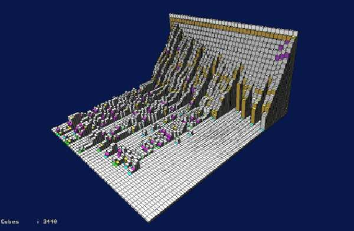
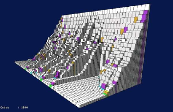
Figure 10: Comparing two search procedures for the 40-queens problem with VRML views computed by trace analysis.

A second experiment is the generation of a 3D variable update view [29]. The evolution of the domains of the variables during the computation is displayed in three dimensions. It gives a tool à la TRIFID [5] (here however colors are introduced to display specific events as in the variable update view of [28]). The trace analyzer makes a VRML file by computing domain size on each tell and reject event, and when a solution is found. The details of reduce events allow us to assign color to each kind of domain update (for example minimum or maximum value removed or domain emptied) as made by Simonis and Aggoun in the Cosytec Search-Tree Visualizer [28]. The trace analysis is implemented in about 125 lines of Prolog and generates an intermediate file. A program implemented in 240 lines of C converts this file into VRML format.

Figure 10 shows the resolution of the 40-queens problem with two different labelling strategies. We have three axes: variables (horizontal axis of the vertical “wall”), domain size (vertical axis) and time. The first strategy is a first-fail selection of the labelled variable and the first value tried is the minimum of its domain. The second strategy is also a first-fail strategy but variable list is sorted with the middle variable first and the middle of domain is preferred to its minimum. This strategy derives from one described by Simonis and Aggoun [28]. This approach allows to compare the efficiency of these two strategies by manipulating the 3D-model. With the first strategy, we get a quick decreasing of the domain size on one side of the chess-board and a long oscillation of the domain size on the other side. With the second strategy, the decreasing of domain size is more regular and more symmetrical, the solution is found faster. In fact, the second strategy, which consists in putting the queens from the center of the chess-board, benefits more from the symmetrical nature of the problem. The possibility of moving manually the figure facilitates observation of such property.

6 Discussion and Conclusion

This article is a first attempt to define new ports for tracing finite domain solvers. We do not claim that the trace model presented here is the ultimate one. On the contrary we propose a methodology to experiment and to improve it. This methodology is based on the following steps: definition of an executable formal model of trace, extraction of relevant informations by a trace analyzer, utilization of the extracted informations in several debugging tools. Each debugging tool extracts from the same generic trace the information it needs.

The formal approach of trace modeling used here allows to clearly define the ports. Then the implementation of the model by a meta-interpreter almost written in ISO-Prolog, a logic programming language with a clear semantics, allows to preserve its correctness wrt the formal model. This methodology is efficient enough on small examples and therefore is of practical interest. However to handle large realistic examples will require hard-coded implementation of the trace model.

Different aspects must be examined to estimate the results. First the formal model itself. Two ports are directly related to logic programming (tell and told) and correspond to the well-known ports call and exit of [3], the others correspond to a small number of different steps of computation of the reduction operator fix-point. On the other side we defined a great number of (possibly large sized) attributes to ensure that each event carries enough potentially useful informations. This immediately shows the limits of our model: it is probably general enough to take into account several finite domain solvers, but tracing the complete behavior of different solvers will require new or different ports to take into account different kinds of control, specific steps of computation (e.g. constraint posting, labelling phase, …), or different algorithms.

The proposed methodology shows the way to progress: defining the trace with a formal model makes easier to compare different trace models. It is thus easier to see which are the missing ports or attributes. Some solvers use a propagation queue with events instead of constraints (in this case new ports or same ports but with different attributes are necessary), or do not use backtracking (then told is never used). The question is also to find the right balance between the number of events and the attributes, in such a way that a hard-coded efficient implementation of (a part of) the trace model is still possible. For example the attribute withdrawn of the port reduce concerns one variable only. Therefore if several variables are involved by a single reduction step, there will be several reduce events. Another possibility would be to have a unique event with a port whose withdrawn attribute includes several variables at once. Gathering too many informations in one event may slow down the tracer considerably. The trace production must be as fast as possible in order to keep the best performances of the solver.

The ports and attributes presented here seem to be a good basis to start the study of a generic trace for clp(fd). In [8] a sample of additional ports are suggested to cope with different finite domain solvers.

The second aspect concerns the extraction of tool specific relevant informations. The generic trace, by definition, contains too many informations if used by a unique debugging tool only. It is also not intended to be stored in a huge file, but it should be filtered on the fly and re-formatted for use by some given tool. The methodology we proposed here, à la opium, is well-known and has been shown to be efficient and general enough to be used in practice also in hard-coded implementations. It allows to specify the trace analysis in a high level language (here Prolog) in a way which is independent from the trace production.

For each experimented tool we have presented here there is a specific analyzer which needs only few lines of code. With this approach, building different views of the same execution requires only to modify the trace analyzer. Notice that the implementation presented here assumes that there is only one trace analyzer running in parallel with the solver. The question of how different analyzers, working simultaneously, could be combined is not considered here.

Finally the third aspect concerns the experimentation. The main challenge in constraint debugging is performance debugging. Our objective is to facilitate the development of constraint resolution analysis tools in a manner which is as independent as possible from the solvers platforms. The three steps method (generic tracer/trace analyzer/debugging tool) is a way to approach such a goal. We experimented it by building several analyzers and (limited) tools very easily, without having to change the trace format. Of course much more experiences are still needed.

Another way to estimate the results of this article is to consider some of the existing debugging tools and to observe that most of the informations relevant for each of these tools are already present in the ports and their attributes. Here are briefly reviewed some platform independent tools, namely debugging tools using graphical interfaces where labelling, constraints and propagation can be visualized.

The Search-Tree Visualization tool for CHIP, described by Simonis and Aggoun [28] displays search-trees, variables and domain evolution. The whole of this information is present in the proposed ports. Our experimentation shows that search-tree and constraints can easily be displayed. The relevant information is also present for the Oz Explorer, a visual programming tool described by Schulte [27], also centered on the search-tree visualization with user-defined displays for nodes. It is also the case in the search-tree abstractor described by Aillaud and Deransart [1] where search-tree are displayed with constraints at the nodes.

In Grace, a constraint program debugger designed by Meier [25], users can get information on domain updates and constraint awakenings. This is available in our trace via our 8 ports. Grace also provides the ability to evaluate expressions using the current domain of the variables. As the domain of the variables is an attribute of all events, it can be obtained by any analyzer of our trace. The CHIP tool also provide update views in which, for example, useless awakenings are visible. In our environment useless awakenings could be detected by a select not followed by a reduce. The visualization tool by Carro and Hermenegildo [5] traces the constraint propagation in 3 dimensions according to time, variable, and cardinal of the domain. The required information is present in our trace. The S-boxes of Goualard and Benhamou [17] structure the propagation in and the display of the constraint store. Structuring the propagation requires to modify the control in the solver. Displaying the store according to the clausal structure would however cause no problem.

An important aspect, not presented in this paper, concerns the possibility of interactive tools. This means that some debugging tools may request to re-execute some already traced execution. Special mechanisms must be involved in order to re-execute efficiently and with the same semantics some part of the execution. How such capability may influences the form of the generic trace is still an open question and will be further investigated.

References

- [1] C. Aillaud and P. Deransart. Towards a language for clp choice-tree visualisation. In Deransart et al. [10], chapter 8.
- [2] F. Benhamou. Interval constraint logic programming. In A. Podelski, editor, Constraint Programming: Basics and Trends, pages 1–21. Springer-Verlag, Lecture Notes in Computer Science 910, 1994.
- [3] L. Byrd. Understanding the control flow of Prolog programs. In S.-A. Tärnlund, editor, Logic Programming Workshop, Debrecen, Hungary, 1980.
- [4] M. Carro and M. Hermenegildo. Tools for search-tree visualisation: The apt tool. In Deransart et al. [10], chapter 9.
- [5] M. Carro and M. Hermenegildo. The vifid/trifid tool. In Deransart et al. [10], chapter 10.
- [6] Y. Caseau, F.-X. Josset, and F. Laburthe. Claire: combining sets, search and rules to better express algorithms. In D. De Schreye, editor, Proc. of the 15th Int. Conference on Logic Programming, pages 245–259. MIT Press, 1999.
- [7] Cosytec. CHIP++ Version 5.2. documentation volume 6. http://www.cosytec.com, 1998.
- [8] Romuald Debruyune, Jean-Daniel Fekete, Narendra Jussien, Mohammad Ghoniem, Pierre Deransart, Ludovic Langevine, and e al. A proposal of concrete format for fracing constraint programming (based on a dtd xml), October 2001. Deliverable D2.2.2.1 (in French).
- [9] P. Deransart, A. Ed-Dbali, and L. Cervoni. Prolog, The Standard; Reference Manual. Springer Verlag, April 1996.
- [10] P. Deransart, M. Hermenegildo, and J. Małuszyński, editors. Analysis and Visualisation Tools for Constraint Programming. Number 1870 in LNCS. Springer Verlag, 2000.
- [11] M. Ducassé. Abstract views of Prolog executions with Opium. In P. Brna, B. du Boulay, and H. Pain, editors, Learning to Build and Comprehend Complex Information Structures: Prolog as a Case Study, Cognitive Science and Technology, chapter 10, pages 223–243. Ablex, 1999.
- [12] M. Ducassé. Opium: An extendable trace analyser for Prolog. The Journal of Logic programming, 39:177–223, 1999. Special issue on Synthesis, Transformation and Analysis of Logic Programs, A. Bossi and Y. Deville (eds).
- [13] M. Ducassé and J. Noyé. Logic programming environments: Dynamic program analysis and debugging. The Journal of Logic Programming, 19/20:351–384, May/July 1994.
- [14] ECLiPSe. Constraint logic programming system. http://www-icparc.doc.ic.ac.uk/eclipse/.
- [15] G. Ferrand, W. Lesaint, and A. Tessier. Value withdrawal explanation in CSP. In M. Ducassé, editor, AADEBUG’00 (Fourth International Workshop on Automated Debugging), pages 188–201, 2000. The COmputer Research Repository (CORR) cs.SE/0012005.
- [16] GNU-Prolog. A clp(fd) system based on Standard Prolog (ISO) developed by D. Diaz. http://gprolog.sourceforge.net/ Distributed under the GNU license.
- [17] F. Goualard and F. Benhamou. Debugging Constraint Programs by Store Inspection. In Deransart et al. [10], chapter 11.
- [18] Y. Gurevitch. Evolving algebras, a tutorial introduction. Bulletin of the European Association for Theoretical Computer Science, 43:264–284, 1991.
- [19] E. Jahier. Collecting graphical abstract views of Mercury program executions. In M. Ducassé, editor, Proceedings of the International Workshop on Automated Debugging (AADEBUG2000), Munich, August 2000. The COmputer Research Repository (CORR) cs.SE/0010038.
- [20] E. Jahier, M. Ducassé, and O. Ridoux. Specifying Prolog trace models with a continuation semantics. In K.-K. Lau, editor, Proc. of LOgic-based Program Synthesis and TRansformation, London, July 2000. Springer-Verlag, Lecture Notes in Computer Science 2042.
- [21] N. Jussien and V. Barichard. The PaLM system: explanation-based constraint programming. In Proceedings of TRICS: Techniques foR Implementing Constraint programming Systems, a post-conference workshop of CP 2000, pages 118–133, Singapore, September 2000.
- [22] E. Koutsofios and S. North. Drawing graphs with dot. TR 910904-59113-08TM, AT&T Bell Laboratories, 1991.
- [23] Ludovic Langevine, Pierre Deransart, Mireille Ducasse, and Ewan Jahier. Tracing and analyzing execution of clp(fd) programs: a trace model and an experimental validation environment. Rr, INRIA, Novembre 2001. Full version of this paper, Public Deliverable D1.2.1, to appear as INRIA/IRISA Research report. http://contraintes.inria.fr/OADymPPaC/.
- [24] K. Marriott and P.J. Stuckey. Programming with Constraints: An Introduction. The MIT Press, Cambridge, Massachussets, 1998.
- [25] M. Meier. Debugging constraint programs. In U. Montanari and F. Rossi, editors, Proceedings of the First International Conference on Principles and Practice of Constraint Programming, number 976 in LNCS, pages 204–221. Springer Verlag, 1995.
- [26] INRIA-Rocquencourt, EMN-Nantes, INSA-Rennes, University of Orléans, Cosytec, and ILOG. Tools for dynamic analysis and development of constraint programs (OADymPPaC), November 2000. An RNTL French Project. http://contraintes.inria.fr/OADymPPaC.
- [27] C. Schulte. Oz Explorer: A Visual Constraint Programming Tool. In Proceedings of the Fourteenth International Conference on Logic Programming (Iclp’97), pages 286–300, Leuven, Belgium, June 1997. The MIT Press.
- [28] H. Simonis and A. Aggoun. Search-Tree Visualisation. In Deransart et al. [10], chapter 7.
- [29] R. Zoumman. Analyse du comportement du solveur de contraintes basée sur la visualisation de traces (in French). Rapport de stage, INRIA, 2001.