Combining Propagation Information and Search Tree Visualization using ILOG OPL Studio

Abstract

In this paper we give an overview of the current state of the graphical features provided by ILOG OPL Studio for debugging and performance tuning of OPL programs or external ILOG Solver based applications. This paper focuses on combining propagation and search information using the Search Tree view and the Propagation Spy. A new synthetic view is presented: the Christmas Tree, which combines the Search Tree view with statistics on the efficiency of the domain reduction and on the number of the propagation events triggered.

Introduction

Built upon the ILOG Views graphical components [8], ILOG OPL Studio was initially intended to provide an Integrated Development Environment for the OPL language (Optimization Programming Language) [16]. Now it can also serve as a debugging environment for external ILOG Solver applications independently of the OPL language. Based on new facilities provided in ILOG Solver 5.0 [11], such as the search monitor and the trace mechanism, ILOG OPL Studio provides tools for graphically visualizing and debugging the execution of an ILOG Solver program. This paper explores both OPL program debugging and pure ILOG Solver application debugging using the ILOG OPL Studio debugger. However, the graphical features presented could be reused with other constraint solvers.

In CP programs there is a two-level architecture consisting of a constraint component and a programming component [16]. The constraint component, also called constraint store, contains the constraints accumulated at a given computation step and provides basic operations that lead to domain reductions by means of constraint propagation. The constraint component is also responsible for maintaining constraint satisfaction and detecting failures. The programming component provides a means of combining the basic operations, often in a non-deterministic way, to guide the solver in the search for a solution. This two-level architecture leads to a two-level visualization. The programmed search part can be visualized as a direct representation of the Search Tree [1, 14]. The constraint propagation can lead to a representation of the impact on the domains of the decision variables [1, 4, 9] and to a trace of the events [5]. This paper focuses on combining propagation and search information. Although ILOG OPL Studio provides several graphical facilities for domain visualization, these features are not presented here. First, we describe the Search Tree visualization. Next, we show how the Propagation Spy represents the propagation events. Finally, we show how to combine search tree and propagation information in terms of both user interaction and integrated visualization. Special attention is paid to providing an interaction mechanism familiar to users of debuggers for traditional languages. A new synthetic view is presented: the Christmas Tree, which combines statistics on domain reduction and propagation events with the Search Tree view.

Visualization of the Search Tree

Different approaches to search tree visualization are possible, from dynamic visualization to post-mortem analysis [14, 1]. We choose the dynamic visualization approach so that we can monitor the exploration order. Because the educational aspect is important in such a tool, and because ILOG Solver exploration strategy is not limited to Depth-First Search (DFS) [12], we should be able to visualize which is the current visited node, in which order the tree is explored and in which state each node currently is. We use colors to indicate the state of the node and a yellow arrow to indicate the current node. When using exploration strategies other than the DFS you can see the yellow arrow jumping in the tree. The possible states of a node are: created but unexplored so far (white), explored (blue), pruned without exploration (black), solution (green), failure (red). When the yellow arrow points to the root, the algorithm is performing the initial domain reduction.

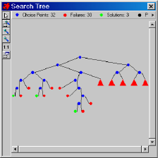
Figure 1: Search Tree visualization for a Golomb Ruler problem with five collapsed subtrees

Tree Reduction

Because the search tree can be very big, ILOG OPL Studio provides ways of obtaining a simplified version of the tree. For instance, it is possible to collapse or expand a subtree. A collapsed subtree is represented by a triangle following the same color conventions as the node representation (Figure 1). Also, OPL constructs provide a way to achieve search tree reduction by abstracting the internal binary tree as an n-ary tree provided that the search procedure contains the forall and tryall OPL keywords. forall is an iterated ”AND” and tryall is an iterated ”OR”, specifying an AND-OR tree [15]. The reduction to the n-ary OR-tree is not obtained by applying abstraction operations on the initial binary tree as exposed in [2] but by means of interlaced goals keeping the information on the true common father of the choices. See Figure 2.

The Choice Stack

Visualizing the shape of the tree is rarely sufficient for program debugging and performance tuning. One needs to know which choice occurred at a specific node and the list of choices made so far in the current branch. This leads to the notion of ”Choice Stack”. In OPL Studio, the Choice Stack is a panel describing the choices made from the root in the current branch. Figure 2 shows the Choice Stack and the Search Tree for a problem of warehouse location [11]. Here, the choices are visible in the form variable = value. After double-clicking on a node in the Search Tree view, the corresponding frames are highlighted in the Choice Stack panel. In Figure 2, the first node below the root is selected and the corresponding frames in the Choice Stack show that the choice at the selected node is the value London set to the variable Supplier[0]. The depth from the root is given between brackets.

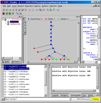
Figure 2: Choice Stack and n-ary Search Tree for a warehouse location problem

Visualization of Propagation Events

Constraint propagation is called before the search and at each Search Tree node. The propagation occurring before the search, at the root node, is called the initial propagation. The ILOG OPL Studio debugger provides a way of displaying the trace of the propagation events and the result of the propagation in terms of domain reduction: the Propagation Spy.

The Propagation Spy

Based on the new Trace mechanism provided in ILOG Solver 5.0 [11], the ILOG OPL Studio debugger provides a panel called the ”Propagation Spy”. This is a special hierarchical sheet containing a tree hierarchy in the first column [8]. Figure 3 shows the initial propagation for the ”Pheasants and Rabbits” problem [3]. Each line is a Propagation Event, such as ”Set Max”, ”Set Value”, ”Post Constraint”, ”Propagate Constraint”, ”Constraint Fail”, etc. Each column contains the impact on one variable. Time passes vertically, from top to bottom. The textual description of the events is appended inside the first column. When an event line is selected the columns are rearranged so that the variables of interest are displayed first. The cell at the junction of an event line and a variable column is colored according to the type of event and shows the result of the event in textual form. Thus, the domain reduction history can be followed here.

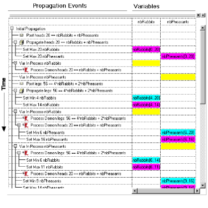
Figure 3: The Propagation Spy for the pheasants and rabbits problem

Because the number of events can be very high, the Propagation Spy is not always active: it is activated on demand by the user. We describe the user interaction in more detail in the next section: Combining Search and Propagation Information. The Propagation Spy is convenient for propagation teaching and for failure analysis. When used with ILOG Solver add-ons such as ILOG Scheduler, a specific trace is inserted in the Propagation Spy [10] so that the program can be debugged at a higher level.

Combining Search and Propagation Information

In this section we will show how the user interacts with the debugger with the two levels of information: the search and the propagation. Then we will propose a synthetic view combining statistical information about the propagation with the search tree.

User interaction with the debugger

We took special care to provide an interaction mechanism familiar to users of debuggers for traditional languages (such as Microsoft Visual Studio, Karmira BugSeeker${}^{\texttt{TM}}$ for Java or dbx on UNIX). In such debuggers, the user can interrupt the execution, step into, out of, or over a function, and restart. In debuggers for traditional languages the function call stack is a common abstraction of the flow of execution, and the current state of the variables can be inspected. Here, in the context of a CP program, these concepts are respectively replaced by the choice stack and the state of the domains. In Figure 4 we propose a specification for user interaction with a CP debugger such as the ILOG OPL Studio debugger and a mapping to traditional debugging concepts in a traditional debugger.

Action	Traditional debugger	CP debugger
Step Into	Step into a function	Step into a node, tracing prop.
Step Out	Step out of a function	Step out of a node, stop tracing prop.
Step Over	Step over a function	Step over a node, or prop. event
Skip Step	Step skipping predefined files	Trace prop. and stop at next node
Break	Break at next instruction	Break at next node or event
Breakpoint	Break at line	Break at node
Current	Current line in the source code	Current visited node
Stack	Function Call Stack	Choice Stack

Figure 4: Concept mapping between a traditional debugger and a CP debugger

When the user launches a first execution, he sees the tree drawing itself in the Search Tree viewer. If necessary, he can interrupt the execution. The debugger stops at the beginning of a node visit. Then, if the user chooses to step into the node, each step is a propagation event. So a line is added to the Propagation Spy at each ”Step Into” command. He can then step out, that is, stop tracing the propagation and continue to the next visited node. Because of the non-deterministic nature of the CP search, it is not possible to draw the tree in advance. A second run is necessary to focus on a segment of the tree. After a first run, the user identifies interesting regions and places a breakpoint at an interesting node. At the second run, the tree nodes are ”laundered”, (i.e. they become white) and then recolored. The debugger stops at the breakpoint, that is, when the corresponding Search Tree node is visited.

A synthetic view: the Christmas Tree

The Search Tree viewer of ILOG OPL Studio provides a way of combining statistics on propagation information with the tree representation. The information added to the tree is the number of propagation events and the effective global domain reduction at each node. It is important to distinguish between these two pieces of information because many propagation events can be triggered with little impact on the domain reduction. The size of the nodes becomes proportional to the number of propagation events fired at each node (which is highly correlated with the time spent at each node). The meaning of the colors remains unchanged, except that the color is lighter or darker depending on the effective domain reduction obtained during the propagation at this node. The Search Tree now has big and small balls with different colors, that is why we call it the ”Christmas Tree”. Figures 11 and 12 represent the Christmas Trees associated with the ”Golomb Ruler” problem [7]. The statistical information connected with the initial propagation is concentrated at the tree root. It becomes obvious that all nodes are not equal. We can detect if, in failure nodes (red nodes), the failure is discovered early (small node) or late (large node).

Principle of Operations

In this section we describe the basic implementation structure of the visual tools and their integration with user applications.

The architecture is a client-server architecture where the GUI is the server and the user application the client. The GUI is loosely coupled with the application. It could be reused with non-ILOG products, provided that the protocol between the GUI and the engine is respected. This protocol is based on XML messages exchanged via sockets. For ILOG based applications, this protocol is encapsulated in a C++ library called ”Debugger Library” which takes care of the communication layer and must be linked to the user application. The API is object-oriented, as is ILOG Solver [13]. The application programmer must implement an IlcDebuggable interface, overriding two virtual methods, stateModel() and solveModel(). He must instantiate an IlcDebugger object passing as arguments the name of the machine and the port number on which the GUI server is listening. The Debugger Library has its own subclasses of the Search Monitor class and of the Propagation Trace class defined in ILOG Solver [11]. These classes have a set of virtual methods for each search and propagation event. The Debugger classes take care of sending the appropriate Propagation and Search information to the GUI, wrapping it in XML messages.

Experimentation

In this section, we will concentrate first on search procedure improvement with the regular Search Tree, using a scheduling problem expressed in OPL. Then, we will show how to use the Christmas Tree and the Propagation Spy to illustrate propagation issues with a pure ILOG Solver sample.

Improving the search

The experimentation for search improvement is based on a Scheduling problem: job-shop 6 [6]. The aim is to schedule a number of jobs on a set of machines to minimize completion time, often called the makespan. Each job is a sequence of tasks and each task requires a machine. Each intermediate solution found by OPL improves the objective function (minimize makespan) while satisfying the other constraints. Figure 6 shows the shape of the tree with the default search procedure of OPL. To begin with, we basically have the intuition that we must pay attention to right subtrees (Figure 5).

Figure 5: Right sub-tree in a binary tree

For a binary tree, if we consider that the right branch is the contradiction of the left branch, when right subtrees are developed one of the following two conclusions can be drawn. Either solutions are found in the right subtree, in which case the search could be improved since it is the contradiction of a choice that leads to a better solution. Or, solutions are not found in the right subtree, which is an indication that the propagation could be improved, because the back propagation of the cost should have pruned the subtree automatically. Therefore, the presence of right subtrees should be monitored. Next, when using the Depth First Search exploration order, the higher in the tree the right subtrees are, the more we should pay attention to them, because the tree is potentially exponential in its depth.

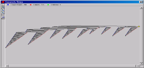
Figure 6: The job-shop 6 problem search tree using the default search procedure of OPL

When we use the default search procedure of ILOG OPL Studio to solve the job-shop 6 problem (with Depth First Search as the exploration order), we notice that right subtrees exist in the higher part of the tree (Figure 6). These right subtrees contain solutions, therefore contradictions of the choices made by the default strategy of OPL lead to better solutions during the minimization process. In scheduling applications with unary resources, the general strategy is to rank each unary resource. Ranking a unary resource consists of finding a total ordering for all activities requiring the resource. Once activities are ordered, a solution can be found efficiently. The detected inefficiency of the default search procedure is due to the fact that it ranks a resource completely before selecting another resource to rank. The default search procedure is not opportunistic enough. The user-defined search procedure in Figure 7 tries to improve that.

search {
  while not isRanked(tool) do
    select(r in 1..6 : not isRanked(tool[r])
                     ordered by increasing nbPossibleFirst(tool[r]))
       select(t in toolTasks[r]
                     : isPossibleFirst(tool[r],task[t.i,t.j])
                     ordered by decreasing dmin(task[t.i,t.j].start))
          tryRankFirst(tool[r],task[t.i,t.j]);
  forall(i in 1..6)
    forall(j in 1..6)
       task[i,j].start = dmin(task[i,j].start);
};

Figure 7: A user-defined search procedure for the job-shop 6 problem

First, we select the resource that has the smallest number of activities we could rank at first position. Then, we select among the tasks requiring this resource that are rankable first, the one which has the earliest starting time. The instruction tryRankFirst(tool[r],task[t.i,t.j]) is nondeterministic and has two alternatives. The first alternative adds the constraint that task[t.i,t.j] be ranked first among the unranked activities of the tool[r] resource. The second alternative (used when backtracking) adds the constraint that task[t.i,t.j] must not be ranked first among the unranked activities of tool[r]. We made a deliberate mistake in the task selection by ordering by latest starting time (decreasing keyword) instead of earliest starting time (increasing keyword). This leads to the Search Tree of Figure 8. The tree is worse in shape, with a lot of right subtrees.

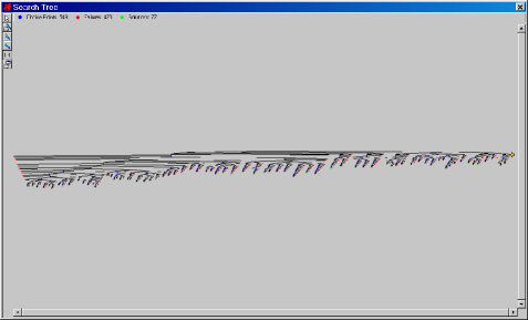
Figure 8: The job-shop 6 problem search tree using a (buggy) user-defined search procedure in OPL

Using the Choice Stack panel, we can identify which choice leads to right subtrees. Then, after ordering by the increasing earliest starting time, the shape of the tree is much better. There are fewer right subtrees and the overall size of the tree is smaller (Figure 9).

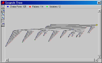
Figure 9: The job-shop 6 problem search tree using an improved user-defined search procedure in OPL

Improving the propagation

The experimentation concerning the propagation improvement is based on the Golomb Ruler problem [7]. The goal is to find a set of values representing the graduations of a rule such that the difference between each pair of graduations is always distinct, and such that the length of the rule is minimal. We use the alldifferent global constraint of ILOG Solver with two different levels of propagation. When using the basic filter level of this constraint, the solver guarantees that, at any computation point, the specified variables do not have the values of the already-assigned variables inside their domain. When using the extended filter level, the solver reasons on the domains instead of the values and guarantees that, for each value in the domain of any given variable, there exist values in the domains of the remaining variables such that the constraint is satisfied. So the extended level enforces a stronger pruning than the basic one.

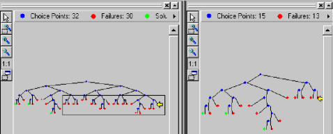
Figure 10: The Golomb problem: on the left the basic filter level, on the right the extended filter level

Figure 10 represents the trees corresponding to the two filter levels. The basic filter level produces a bigger tree with additional right subtrees as compared to the extended filter level. These right subtrees have only failure leaves, a sign of lack of propagation. By just setting the filter level to the extended level these right subtrees are pruned. But does this mean that we saved time ? Here, the Christmas Tree gives us a picture of the cost and of the efficiency of this extended propagation.

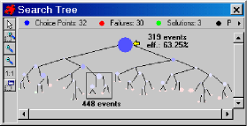
Figure 11: Christmas Tree for the Golomb 6 problem with basic level of propagation for the alldifferent constraint

Let us compare the number of propagation events in the first right subtree located in the frame in Figure 11 with the number of propagation events occurring at the corresponding big failure node in Figure 12. We see that the big node required two times fewer propagation events for detecting failure than the subtree. So, yes, the extended propagation saved time here. Yet, if we compare the initial propagation statistics by looking at the root node, we see that the efficiency of domain reduction is the same (63.25%). The extended propagation level triggered a few more events but with no result.

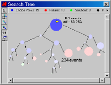
Figure 12: Christmas Tree for the Golomb 6 problem with extended level of propagation for the alldifferent constraint

Now, let us enter into the details by using the Propagation Spy. By inspecting the Initial Propagation, we can see that the solver adds a hidden constraint when posting the alldifferent constraint. When tracing the propagation at the first big failure node of the extended filter level and comparing to the corresponding node of the basic filter level the Propagation Spy detects the extra propagation (Figure 13). On the left, with the basic filter level, the propagation stops after reducing the variable difference[11] to the interval 7..11. On the right, with the extended level, the propagation of an additional internal constraint posted by the allDifferent constraint strongly reduces the domains by means of ”Set Min” events. This additional propagation leads to a failure, avoiding a subtree exploration.

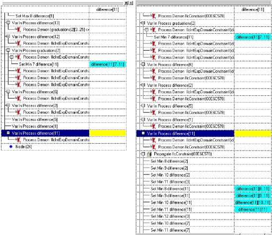
Figure 13: Comparing two Propagation traces using the Propagation Spy for the Golomb 6 problem (on the left, basic filter level, on the right, extended filter level)

However, by inspecting in detail we see that four ”Set Min” events are triggered on the difference[11] variable where one should suffice. These ”Set Min” events are ”Remove Value” orders that have been translated by the solver into ”Set Min” because the value to remove was a bound. Then, we have the intuition that reasoning on bounds instead of on domains should be sufficient. If we tune the alldifferent constraint to the intermediate filter level, which reasons on bounds instead of on domains, we obtain the same search tree as compared to the extended filter level. The Propagation Spy shows that the difference[11] variable at the same Choice Point is bound more quickly (Figure 14).

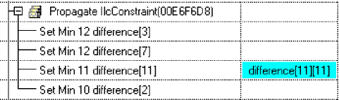
Figure 14: Propagation Spy for the Golomb 6 problem with intermediate filter level

Conclusion

We have presented an overview of the current state of the ILOG OPL Studio debugger capabilities for performance tuning of CP programs. The experimentation on improving the search procedure with the Search Tree visualization is promising. A graphic trace of the propagation events, in order to better understand the inner details of what happens at each node, has also been presented. Combining the two pieces of information by adding statistics on the ”weight” of each node in the Christmas Tree seems to be an important step toward visualizing where the time is spent.

Acknowledgments

We would like to thank Laurent Perron for his help on the ILOG Solver search monitor and Jean-Charles Régin and Xavier Nodet for their explanations of the ILOG Solver and ILOG Scheduler trace mechanism. We would also like to thank Michel Leconte, Philippe Laborie and Veronica Murphy for their comments and ideas.

References

- [1] Abder Aggoun and Helmut Simonis. Search tree visualization. In Pierre Deransart, Manuel V. Hermenegildo, and Jan Maluszynski, editors, Analysis and Visualization Tools for Constraint Programming, volume 1870 of Lecture Notes in Computer Science, pages 191–208. Springer, 2000.
- [2] Christophe Aillaud and Pierre Deransart. Towards a language for CLP choice-tree visualisation. In Pierre Deransart, Manuel V. Hermenegildo, and Jan Maluszynski, editors, Analysis and Visualization Tools for Constraint Programming, volume 1870 of Lecture Notes in Computer Science, pages 209–236. Springer, 2000.
- [3] Bull. Manuel Charme First, Guide d’utilisation et manuel de référence. Bull S.A., Septembre 1991.
- [4] Manuel Carro and Manuel Hermenegildo. Tools for constraint visualisation: The vifid/trifid tool. In Pierre Deransart, Manuel V. Hermenegildo, and Jan Maluszynski, editors, Analysis and Visualization Tools for Constraint Programming, volume 1870 of Lecture Notes in Computer Science, pages 253–270. Springer, 2000.
- [5] Mireille Ducassé. Opium: An extendable trace analyser for prolog. The Journal of Logic Programming, special issue on Synthesis, Transformation and Analysis of Logic Programs, 1999. A. Bossi and Y. Deville (eds).
- [6] H. Fisher and G. L. Thompson. Probabilistic learning combinations of local job-shop scheduling rules. In J. F. Muth and G. L. Thompson, editors, Industrial Scheduling, pages 225–251. Prentice Hall, Englewood Cliffs, New Jersey, 1963.
- [7] S. W. Golomb. Shift Register Sequences. Aegean Park Press, Laguna Hills, 1982.
- [8] ILOG. Views 3.1 Reference Manual, volume II. ILOG, April 1999.
- [9] ILOG. OPL Studio 3.5 User’s Manual. ILOG, 2001.
- [10] ILOG. Scheduler 5.1 Reference Manual. ILOG, 2001.
- [11] ILOG. Solver 5.1 Reference Manual. ILOG, 2001.
- [12] Laurent Perron. Search procedures and parallelism in constraint programming. In Joxan Jaffar, editor, Proceedings of the Fifth International Conference on Principles and Practice of Constraint Programming (CP99), pages 346–360. Springer-Verlag, 1999.
- [13] Jean-Francois Puget and Michel Leconte. Beyond the glass box: Constraints as objects. In International Logic Programming Symposium, pages 513–527, 1995.
- [14] Christian Schulte. Oz Explorer: A visual constraint programming tool., pages 286–300. ICLP’97. Lee Naish, editor, Leuven, Belgium, the MIT press edition, July 1997.
- [15] Pascal Van Hentenryck, Laurent Perron, and Jean-Francois Puget. Search and strategies in OPL. ACM Transactions on Computational Logic, 1(2):pages 282–315, October 2000.
- [16] Pascal Van Hentenryck, with contributions by Irvin Lustig Laurent Michel, and Jean-Francois Puget. The OPL Optimization Programming Language. MIT Press, 1999.