Dense Point Sets Have Sparse Delaunay Triangulations
or “…But Not Too Nasty”

Abstract

The spread of a finite set of points is the ratio between the longest and shortest pairwise distances. We prove that the Delaunay triangulation of any set of $n$ points in $\mathbb{R}^{3}$ with spread $\Delta$ has complexity $O(\Delta^{3})$. This bound is tight in the worst case for all $\Delta=O(\sqrt{n})$. In particular, the Delaunay triangulation of any dense point set has linear complexity. We also generalize this upper bound to regular triangulations of $k$-ply systems of balls, unions of several dense point sets, and uniform samples of smooth surfaces. On the other hand, for any $n$ and $\Delta=O(n)$, we construct a regular triangulation of complexity $\Omega(n\Delta)$ whose $n$ vertices have spread $\Delta$.

1 Introduction

Delaunay triangulations and Voronoi diagrams are one of the most thoroughly studied objects in computational geometry, with applications to nearest-neighbor searching [4, 31, 36, 65], clustering [2, 70, 72, 87], finite-element mesh generation [29, 47, 74, 90], deformable surface modeling [28], and surface reconstruction [7, 8, 9, 10, 20, 69]. Many algorithms in these application domains begin by constructing the Delaunay triangulation or Voronoi diagram of a set of points in $\mathbb{R}^{3}$. Since three-dimensional Delaunay triangulations can have complexity $\Omega(n^{2})$ in the worst case, these algorithms have worst-case running time $\Omega(n^{2})$. However, this behavior is almost never observed in practice except for highly-contrived inputs. For all practical purposes, three-dimensional Delaunay triangulations appear to have linear complexity.

This frustrating discrepancy between theory and practice motivates our investigation of practical geometric constraints that imply low-complexity Delaunay triangulations. Previous research on this topic has focused on random point sets under various probability distributions [18, 76, 58, 78, 40, 39, 52, 59, 62]; well-spaced point sets, which are low-discrepancy samples of Lipschitz density functions [29, 74, 79, 80, 92, 93]; and surface samples with various density constraints [11, 12, 52, 59, 62]. (We will discuss the connections between these models and our results in Section 2.) Our efforts fall under the rubric of realistic input models, which have been primarily studied for inputs consisting of polygons or polyhedra [16, 100, 101] or sets of balls [66, 101].

This paper investigates the complexity of three-dimensional Delaunay triangulations in terms of a geometric parameter called the spread, continuing our work in an earlier paper [52]. The spread of a set of points is the ratio between the largest and smallest interpoint distances. Of particular interest are dense point sets in $\mathbb{R}^{d}$, which have spread $O(n^{1/d})$. Valtr and others [6, 49, 96, 97, 98, 99] have established several combinatorial results for dense point sets that improve corresponding bounds for arbitrary point sets. For example, a dense point set in $\mathbb{R}^{3}$ has at most $O(n^{7/3})$ halving planes; the best upper bound known for arbitrary point sets is $O(n^{5/2})$ [89]. For other combinatorial and algorithmic results related to spread, see [5, 23, 33, 55, 63, 64, 71].

In Section 3, we prove that the Delaunay triangulation of any set of points in $\mathbb{R}^{3}$ with spread $\Delta$ has complexity $O(\Delta^{3})$. This upper bound is independent of the number of points in the set. In particular, the Delaunay triangulation of any dense point set in $\mathbb{R}^{3}$ has only linear complexity. This bound is tight in the worst case for all $\Delta=O(\sqrt{n})$ and improves our earlier upper bound of $O(\Delta^{4})$ [52].

Our upper bound can be extended in several ways. To make the notion of spread less sensitive to close pairs, we define the order-$k$ spread $\Delta_{k}$ to be the ratio of the diameter of the set to the radius of the smallest ball containing $k$ points. Our proof almost immediately implies that the Delaunay triangulation has complexity $O(k^{2}\Delta_{k}^{3})$ for any $k$. Our techniques also generalize fairly easily to regular triangulations of disjoint balls whose centers have spread $\Delta$. With somewhat more effort, we show that if a set of points can be decomposed into $k$ subsets, each with spread $\Delta$, then its Delaunay triangulation has spread $O(k^{2}\Delta^{3})$. Our results also imply upper bounds on the complexity of the Delaunay triangulation of uniform or random samples of surfaces. Finally, our combinatorial bounds imply that the standard randomized incremental algorithm [65] constructs the Delaunay triangulation any set of points in expected time $O(\Delta^{3}\log n)$. These and other related results are developed in Section 4.

However, our upper bound does not generalize to arbitrary triangulations. In Section 5, for any $n$ and $\Delta\leq n$, we construct a regular triangulation, whose $n$ vertices have spread $\Delta$, whose overall complexity is $\Omega(n\Delta)$. (The defining balls for this triangulation overlap heavily.) This worst-case lower bound was already known for Delaunay triangulations for all ${\sqrt{n}\leq\Delta\leq n}$ [52]. In particular, there is a dense point set in $\mathbb{R}^{3}$, arbitrarily close to a cubical lattice, with a regular triangulation of complexity $\Omega(n^{4/3})$.

Throughout the paper, we analyze the complexity of three-dimensional Delaunay triangulations by counting their edges. Since the link of every vertex in a three-dimensional triangulation is a planar graph, Euler’s formula implies that any triangulation with $n$ vertices and $e$ edges has at most $2e-2n$ triangles and $e-n$ tetrahedra. Two points are joined by an edge in the Delaunay triangulation of a set $S$ if and only if they lie on a sphere with no points of $S$ in its interior.

2 Previous and related results

2.1 Points in Space

Our results for dense sets compare favorably with three other types of ‘realistic’ point data: points with small integer coordinates, random points, and well-spaced points. Figure 1 illustrates these four models. Although the results for these models are quite similar, we emphasize that with one exception—integer points with small coordinates are dense—results in each model are formally incomparable with results in any other model.

Unlike our new results, which apply only to points in $3$-space, all of these related results have been generalized to higher dimensions. We conjecture that the Delaunay triangulation of any $d$-dimensional point set with spread $\Delta$ has complexity $O(\Delta^{d})$, but new proof techniques will be required to prove this bound.

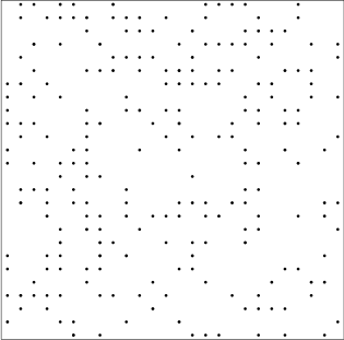
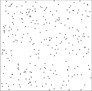
(a)	(b)
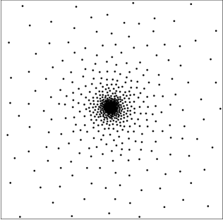
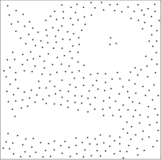
(c)	(d)

Figure 1: Four models of ‘realistic’ point sets. (a) Small integer. (b) Random. (c) Well-spaced. (d) Dense.

Integer points.

First, we easily observe that any triangulation of $n$ points in $\mathbb{R}^{3}$ with integer coordinates between $1$ and $\Delta$ has complexity $O(\Delta^{3})$, since each tetrahedron has volume at least $1/6$. (It is an open question whether this bound is tight for all $n$ and $\Delta$.) In particular, if $\Delta=O(n^{1/3})$, so that the set is dense, the complexity of the Delaunay triangulation is $O(n)$. Dense sets obviously need not lie on a coarse integer grid; nevertheless, this observation provides some useful intuition for our results.

Random points.

Statistical properties of Voronoi diagrams of random points have been studied for decades, much longer than any systematic algorithmic development. In the early 1950s, Meijering [76] proved that for a homogeneous Poisson process in $\mathbb{R}^{3}$, the expected number of Delaunay neighbors of any point is $48\pi^{2}/35+2\approx 15.54$; see Miles [78]. This result immediately implies that the Delaunay triangulation of a sufficiently dense random periodic point set has linear expected complexity. See Møller [82] for generalizations to arbitrary dimensions and Okabe et al. [86, Chapter 5] for an extensive survey of statistical properties of random Voronoi diagrams and Delaunay triangulations.

Bentley et al. [14] proved that for $n$ uniformly distributed points in the $d$-dimensional hypercube, the expected number of points with more than a constant number of Delaunay neighbors is $O(n^{1-1/d}\log n)$; all such points lie near the boundary of the cube. Extending their technique, Bernal [18] proved that the expected complexity of the Delaunay triangulation of $n$ random points in the three-dimensional cube is $O(n)$. Dwyer [40, 39] showed that if a set of $n$ points is generated uniformly at random in the unit ball in $\mathbb{R}^{d}$, the Delaunay triangulation has expected complexity $d^{O(d)}n$; in particular, each point has $d^{O(d)}$ Delaunay neighbors on average.

Random point sets are not dense, even in expectation. Let $S$ be a set of $n$ points, generated independently and uniformly from the unit hypercube in $\mathbb{R}^{d}$. A straightforward ‘balls and bins’ argument [50, 83] implies that the expected spread of $S$ is $\Theta(n^{2/d})$; moreover, with high probability, the spread of $S$ is between $\Omega(n^{2/d}/\log^{\varepsilon}n)$ and $O(n^{2/d+\varepsilon})$ for any $\varepsilon$.

Well-spaced points.

Miller, Talmor, Teng and others [79, 80, 92, 93] have derived several results for well-spaced point sets in the context of high-quality mesh generation. A point set $S$ in $\mathbb{R}^{3}$ is well-spaced with respect to a $1$-Lipschitz spacing function $\lambda:\mathbb{R}^{3}\to\mathbb{R}^{+}$ if, for some fixed constants $0<\delta<1/2$ and $0<\varepsilon<1$, the distance from any point $x\in\mathbb{R}^{3}$ to its second nearest neighbor $p\in S$ is between $\delta\varepsilon\lambda(p)$ and $\varepsilon\lambda(p)$. In her thesis, Talmor [92] proves that Delaunay triangulations of well-spaced point sets have complexity $O(n)$; in particular, any point in a well-spaced point set has $O(1)$ Delaunay neighbors.

Any point set that is well-spaced with respect to a constant spacing function is dense. In general, however, the spread of a well-spaced set can be exponentially large; consider the one-dimensional well-spaced set $\{2^{-i}\mid 1\leq i\leq n\}$. On the other hand, dense point sets can contain large gaps and thus are not necessarily well-spaced with respect to any Lipschitz spacing function; compare Figures 1(c) and 1(d).

Talmor’s linear upper bound [92] depends exponentially on the spacing parameters $\delta$ and $\varepsilon$, but this is largely an artifact of the generality of her results. For the three-dimensional case, we can derive tighter bounds as follows. Let $S$ be a point set in $\mathbb{R}^{3}$ that is well-spaced with respect to some $1$-Lipschitz spacing function $\lambda$. Let $p$ be any point in $S$, and let $q$ and $r$ be any two Delaunay neighbors of $p$. We immediately have the inequalities $\mathopen{|}pq\mathclose{|}\leq\min\{\varepsilon\lambda(p),\varepsilon\lambda(q)\}$ and $\mathopen{|}qr\mathclose{|}\geq\delta\varepsilon\lambda(q)$. Because the spacing function $\lambda$ is Lipschitz, we have $\lambda(q)\geq\lambda(p)-\mathopen{|}pq\mathclose{|}\geq\lambda(p)-\varepsilon\lambda(q)$, which implies that $\lambda(q)\geq\lambda(p)/(1+\varepsilon)$. Together, these inequalities imply that the set of Delaunay neighbors of $p$ has spread at most $2(1+\varepsilon)/\delta=O(1/\delta)$. A packing argument in our earlier paper [52] now implies that $p$ has $O(1/\delta^{2})$ Delaunay neighbors. It follows that the Delaunay triangulation of $S$ has complexity $O(n/\delta^{2})$. (Surprisingly, this bound does not depend on $\varepsilon$ at all!)

Finally, in contrast to both random and well-spaced point sets, a single point in a dense set in $\mathbb{R}^{3}$ can have $\Theta(\Delta^{2})=\Theta(n^{2/3})$ Delaunay neighbors in the worst case [52]. Thus, our upper bound proof must consider global properties of the Delaunay triangulation.

2.2 Points on Surfaces

The complexity of Delaunay triangulations of points on two-dimensional surfaces in space has also been studied, largely due to the recent proliferation of Delaunay-based surface reconstruction algorithms [7, 8, 9, 10, 20, 69]. Upper and lower bounds range from linear to quadratic, depending on exactly how the problem is formulated. Specifically, the results depend on whether the surface is considered fixed or variable, whether the surface is smooth or polyhedral, and on the precise sampling conditions to be analyzed. We first review some standard terminology.

Let $\Sigma$ be a $C^{2}$ surface embedded in $\mathbb{R}^{3}$. A medial ball of $\Sigma$ is a ball whose interior is disjoint from $\Sigma$ and whose boundary touches $\Sigma$ at more than one point. The center of a medial ball is called a medial point, and the closure of the set of medial points is the medial axis of $\Sigma$. The local feature size of a point $x\in\Sigma$, denoted $\operatorname{lfs}(x)$, is the the distance from $x$ to the medial axis. Finally, a set of points $P\subset\Sigma$ is an $\varepsilon$-sample of $\Sigma$ if the distance from any surface point $x\in\Sigma$ to the nearest sample point in $P$ is at most $\varepsilon\cdot\operatorname{lfs}(x)$. This condition imposes a lower bound on the number of sample points in any region of the surface. Given an $\varepsilon$-sample of an unknown surface $\Sigma$, for sufficiently small $\varepsilon$, the algorithms cited above provably reconstruct a surface geometrically close and topologically equivalent to $\Sigma$. As a first step, each algorithm constructs the Voronoi diagram of the sample points; the complexity of this Voronoi diagram is clearly a lower bound on the running time of the algorithm.

Unfortunately, $\varepsilon$-samples can have arbitrarily complex Delaunay triangulations due to oversampling. Specifically, for any surface other than the sphere and any sampling density $\varepsilon>0$, there is an $\varepsilon$-sample whose Delaunay triangulation has complexity $\Theta(n^{2})$, where $n$ is the number of sample points [52]. Thus, in order to obtain nontrivial upper bounds, we must also impose an upper bound on the density of samples.

Dey, Funke, and Ramos [37, 54] define a set of points $P\subset\Sigma$ to be a locally uniform sample of $\Sigma$ if $P$ is well-spaced (in the sense of Miller et al.) with respect to some $1$-Lipschitz function $\lambda:\Sigma\to\mathbb{R}^{+}$ such that $\lambda(x)\leq\operatorname{lfs}(x)$ for all $x\in\Sigma$. If $P$ is well-spaced with respect to the local feature size function, which is always $1$-Lipschitz, we call $P$ a uniform sample of $\Sigma$ [52]. Dey et al. [37] described an algorithm to reconstruct a surface from a locally uniform sample in $O(n\log n)$ time; Funke and Ramos later showed to how extract a locally uniform $\varepsilon$-sample from an arbitrary $\varepsilon$-sample in $O(n\log n)$ time. Neither of these algorithms constructs the Delaunay triangulation of the points.

In our earlier paper [52], we derived lower bounds on the complexity of Delaunay triangulations of uniform samples in terms of the sample measure

$$\mu(\Sigma)=\iint_{\Sigma}\frac{dx^{2}}{\operatorname{lfs}(x)^{2}}.$$

Any uniform $\varepsilon$-sample of $\Sigma$ contains $\Theta(\varepsilon^{2}\mu(\Sigma))$ points. There are smooth connected surfaces with sample measure $\mu$ for which the Delaunay triangulation of any uniform $\varepsilon$-sample has complexity $\Omega(\mu^{2}/\log^{2}\mu)$.

More positive results can be obtained by considering the surface to be fixed and considering the asymptotic complexity of the Delaunay triangulation as the number of sample points tends to infinity. In this context, hidden constants in the upper bounds depend on geometric parameters of the fixed surface, such as the number of facets or their maximum aspect ratio for polyhedral surfaces, or the minimum curvature radius or sample measure for curved surfaces. Since the surface is fixed, all such parameters are considered constants.

Golin and Na [59, 60, 61] proved that if $n$ points are chosen uniformly at random on the surface of any fixed three-dimensional convex polytope, the expected complexity of their Delaunay triangulation is $O(n)$. Using similar techniques, they recently showed that a random sample of a fixed nonconvex polyhedron has Delaunay complexity $O(n\log^{4}n)$ with high probability [62]. In fact, their analysis applies to any fixed set of disjoint triangles in $\mathbb{R}^{3}$.

Attali and Boissonnat [12] recently proved that the Delaunay triangulation of any $(\varepsilon,\kappa)$-sample of a fixed polyhedral surface has complexity $O(\kappa^{2}n)$, improving their previous upper bound of $O(n^{7/4})$ (for constant $\kappa$) [11]. A set of points is called an $(\varepsilon,\kappa)$-sample of a surface $\Sigma$ if every ball of radius $\varepsilon$ whose center lies on $\Sigma$ contains at least one and at most $\kappa$ points in $P$. A simple application of Chernoff bounds (see Theorem 4.11) implies that a random sample of $n$ points on a fixed surface is an $O(\varepsilon,O(\log n))$-sample with high probability, where $\varepsilon=O(\sqrt{(\log n)/n})$. Thus, Attali and Boissonnat’s result improves Golin and Na’s high-probability bound for random points to $O(n\log^{2}n)$.

Our new upper bound has a similar corollary. Informally, a uniform sample of any fixed (not necessarily polyhedral, smooth, or convex) surface has spread $O(\sqrt{n})$, so its Delaunay triangulation has complexity $O(n^{3/2})$. This bound is tight in the worst case; a right circular cylinder with constant height and radius has a uniform $(\varepsilon,1)$-sample with Delaunay complexity $\Omega(n^{3/2})$. Similar arguments establish upper bounds of $O(\kappa^{2}n^{3/2})$ for $(\varepsilon,\kappa)$-samples and $O(n^{3/2}\log^{3/2}n)$, with high probability, for random samples. We describe these results more formally in Section 4.

3 Sparse Delaunay Triangulations

In this section, we prove the main result of the paper.

Theorem 3.1

The Delaunay triangulation of any finite set of points in $\mathbb{R}^{3}$ with spread $\Delta$ has complexity $O(\Delta^{3})$.

Our proof is structured as follows. We will implicitly assume that no two points are closer than unit distance apart, so that spread is synonymous with diameter. Two sets $P$ and $Q$ are well-separated if each set lies inside a ball of radius $r$, and these two balls are separated by distance $2r$. Without loss of generality, we assume that the balls containing $P$ and $Q$ are centered at points $(0,0,2r)$ and $(0,0,-2r)$, respectively. Our argument ultimately reduces to counting the number of crossing edges—edges in the Delaunay triangulation of $P\cup Q$ with one endpoint in each set. See Figure 2.

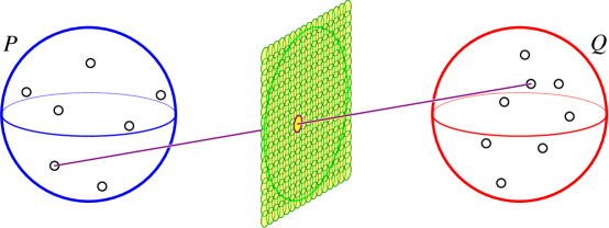
Figure 2: A well-separated pair of sets $P\cup Q$ and a crossing edge intersecting a pixel.

Our proof has four major steps, each presented in its own subsection.

• We place a grid of $O(r^{2})$ circular pixels of constant radius $\varepsilon$ on the plane $z=0$, so that every crossing edge passes through a pixel. In Section 3.1, we prove that all the crossing edges stabbing any single pixel lie within a slab of constant width between two parallel planes. Our proof relies on the fact that the edges of a Delaunay triangulation have a consistent depth order from any viewpoint [42].

• We say that a crossing edge is relaxed if its endpoints lie on an empty sphere of radius $O(r)$. In Section 3.2, we show that at most $O(r)$ relaxed edges pass through any pixel, using a generalization of the ‘Swiss cheese’ packing argument used to prove our earlier $O(\Delta^{4})$ upper bound [52]. This implies that there are $O(r^{3})$ relaxed crossing edges overall.

• In Section 3.3, we show that there are a constant number of conformal (i.e., sphere-preserving) transformations that change the spread of $P\cup Q$ by at most a constant factor, such that every crossing edge of $P\cup Q$ is a relaxed Delaunay edge in at least one image. The proof uses a packing argument in a particular subspace of the space of three-dimensional Möbius transformations. It follows that $P\cup Q$ has at most $O(r^{3})$ crossing edges.

• Finally, in Section 3.4, we count the Delaunay edges for an arbitrary point set $S$ using an octtree-based well-separated pair decomposition [22]. Every edge in the Delaunay triangulation of $S$ is a crossing edge of some subset pair in the decomposition. However, not every crossing edge is a Delaunay edge; a subset pair contributes a Delaunay edge only if it is close to a large empty witness ball. We charge the pair’s $O(r^{3})$ crossing edges to the $\Omega(r^{3})$ volume of this ball. We choose the witness balls so that any unit of volume is charged at most a constant number of times, implying the final $O(\Delta^{3})$ bound.

3.1 Nearly Concurrent Crossing Edges Are Nearly Coplanar

The first step in our proof is to show that the crossing edges intersecting any pixel are nearly coplanar. To do this, we use an important fact about depth orders of Delaunay triangulations, related to shellings of convex polytopes.

Let $x$ be a point in $\mathbb{R}^{3}$, called the viewpoint, and let $S$ be a set of line segments (or other convex objects). A segment $s\in S$ is behind another segment $t\in S$ with respect to $x$ if $t$ intersects $\operatorname{conv}\{x,s\}$. If the transitive closure of this relation is a partial order, any linear extension is called a consistent depth order of $S$ with respect to $x$. Otherwise, $S$ contains a depth cycle—a sequence of segments $s_{1},s_{2},\dots,s_{k}$ such that every segment $s_{i}$ is directly behind its successor $s_{i+1}$ and $s_{k}$ is directly behind $s_{1}$. De Berg et al. [17] describe an algorithm that either computes a depth order or finds a depth cycle for a given set of $n$ segments, in $O(n^{4/3+\varepsilon})$ time. See de Berg [15] and Chazelle et al. [27] for related results.

We say that three line segments form a screw if they form a depth cycle from some viewpoint. See Figure 3(a).

Lemma 3.2

The edges of any Delaunay triangulation have a consistent depth order from any viewpoint. In particular, no three Delaunay edges form a screw.

• Let $x$ be a point, and let $S$ be a sphere with radius $r$ and center $c$. The power distance from $x$ to $S$ is $\mathopen{|}xc\mathclose{|}^{2}-r^{2}$; if $x$ is outside $S$, this is the square of the distance from $x$ to $S$ along a line tangent to $S$. Edelsbrunner [42, 44] proved that a consistent depth order for the simplices in any Delaunay triangulation, with respect to any viewpoint $x$, can be obtained by sorting the power distances from $x$ to the (empty) circumspheres of the simplices. (See Section 4.3.) This is precisely the order in which the Delaunay tetrahedra are computed by Seidel’s shelling convex hull algorithm [88]. We can easily extract a consistent depth order for the Delaunay edges from this simplex order.  ${\square}$

The next lemma describes sufficient (but not necessary) conditions for three pairwise-skew segments to form a screw.

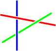
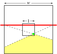
(a) (b)

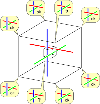
(c)

Figure 3: (a) A screw. (b) Front view of $C$, showing viewpoints where $s_{x}$ appears behind $s_{z}$. (c) Every vertex of $C$ sees a different depth order, two of which are inconsistent. See Lemma 3.3.

Lemma 3.3

Let $c$ be a parallelepiped centered at the origin, and let $C=w\cdot c$ for some $w\geq 2+\sqrt{5}\approx 4.2361$. Three line segments, each parallel to a different edge of $c$, form a screw if they all intersect $c$ but none of their endpoints lie inside $C$.

• Since any affine image of a screw is also a screw, it suffices to consider the case where $c$ and $C$ are concentric axis-aligned cubes of widths $1$ and $w$, respectively. Let $s_{x},s_{y},s_{z}$ be the three segments, parallel to the $x$-, $y$-, and $z$-axes, respectively. Any ordered pair of these segments, say $(s_{z},s_{x})$, define an unbounded polyhedral region $V_{xz}$ of viewpoints from which $s_{x}$ appears behind $s_{z}$. The segment $s_{z}$ is the only bounded edge of $V_{xz}$, and both of its endpoints are outside $C$. Thus, we can determine which vertices of $C$ lie inside $V_{xz}$ by considering the projection to the $xy$-plane. From Figure 3(b), we observe that if $w\geq 2+\sqrt{5}$, then $V_{xz}$ contains exactly half of the vertices of $C$, all with the same $y$-coordinate. A symmetric argument implies that the other four vertices lie in $V_{zx}$. Similarly, $V_{xy}$ and $V_{yx}$ partition the vertices of $C$ by their $z$-coordinates, and $V_{yz}$ and $V_{zy}$ partition the vertices of $C$ along their $x$-coordinates. Thus, each of the eight vertices of $C$ sees one of the eight possible depth orders of the three segments. Since only six of these orders are consistent, two vertices of $C$ see a depth cycle, implying that the segments form a screw. See Figure 3(c).  ${\square}$

Recall that a pixel is a circle of radius $\varepsilon$ in the $xy$-plane.

Lemma 3.4

The crossing edges passing through any pixel lie inside a slab of width $(20+9\sqrt{5})\varepsilon\approx 40.1246\varepsilon$ between two parallel planes.

• We will in fact prove a stronger statement. Any two planes $h_{1}$ and $h_{2}$ whose line of intersection lies in the $xy$-plane define an anchored double wedge, consisting of all the points above $h_{1}$ and below $h_{2}$ or vice versa. We define the thickness of an anchored double wedge to be the width of the two-dimensional slab obtained by intersecting the double wedge with the plane $z=r$. We claim that the crossing edges passing through any pixel lie inside an $\varepsilon$-neighborhood of an anchored double wedge with thickness $(6+3\sqrt{5})\varepsilon$. The lemma follows immediately from this claim.

  Without loss of generality, suppose the pixel $\pi$ is centered at the origin, and let $E$ denote the set of crossing edges passing through $\pi$. Translate each edge in $E$ parallel to the $xy$-plane so that it passes through the origin, and call the resulting set of segments $\tilde{E}$. We need to show that the segments $\tilde{E}$ lie in an anchored double wedge of thickness $(6+3\sqrt{5})\varepsilon$. Since all these segments pass through the origin, it suffices to show that the intersection points between $\tilde{E}$ and the plane $z=r$ lie in a two-dimensional strip of width $(6+3\sqrt{5})\varepsilon$ between two parallel lines. The width of a set of planar points is determined by only three points, so it suffices to check every triple of segments in $\tilde{E}$.

  Let $e_{1},e_{2},e_{3}$ be three arbitrary crossing edges in $E$, and let $\tilde{e}_{1},\tilde{e}_{2},\tilde{e}_{3}$ be the corresponding segments in $\tilde{E}$. For each $i$, let $p_{i}$ and $q_{i}$ be the intersection points of $\tilde{e}_{i}$ with the planes $z=r$ and $z=-r$, respectively, and let $s_{i}\subseteq\tilde{e}_{i}$ be the segment between $p_{i}$ and $q_{i}$. Finally, let $\omega$ be the width of the thinnest two-dimensional strip containing the triangle $\triangle p_{1}p_{2}p_{3}$. Observe that $\triangle$ contains a circle of radius $\omega/3$.

  Let $C$ denote the scaled Minkowski sum $(s_{1}+s_{2}+s_{3})/3$; this is a parallelepiped centered at the origin, with edges parallel to the original crossing edges $e_{i}$. Since each segment $s_{i}$ fits exactly within the slab $-r\leq z\leq r$, so does the cuboid $C$. The intersection of $C$ with the $xy$-plane is the scaled Minkowski sum $(\triangle p_{1}p_{2}p_{3}+\triangle q_{1}q_{2}q_{3})/2$; this hexagon also contains a circle of radius $\omega/3$.

  Let $c$ be the smallest parallelepiped similar to and concentric with $C$ that contains the pixel $\pi$. Since $\pi$ is a circle of radius $\varepsilon$ in the $xy$-plane, $C$ is at least a factor of $\omega/3\varepsilon$ larger than $c$. Lemma 3.2 implies that the Delaunay edges $e_{1},e_{2},e_{3}$ cannot form a screw. Thus, by Lemma 3.3, we must have $\omega/3\varepsilon<2+\sqrt{5}$, or equivalently, $\omega<(6+3\sqrt{5})\varepsilon$, as claimed.  ${\square}$

3.2 Slabs Contain Few Relaxed Edges

At this point, we would like to argue that any slab of constant width contains only $O(r)$ crossing edges. Unfortunately, this is not true—a variant of our helix construction [52] implies that a slab can contain up to $\Omega(r^{3})$ edges, $\Omega(r^{2})$ of which can pass through a single, arbitrarily small pixel. However, most of these Delaunay edges have extremely large empty circumspheres.

We say that a crossing edge is relaxed if its endpoints lie on the boundary of an empty ball with radius less than $4r$, and tense otherwise. In this section, we show that few relaxed edges pass through any pixel. Once again, recall that that $\varepsilon$ denotes the pixel radius.

Lemma 3.5

If $\varepsilon<1/16$, then for any pixel $\pi$, each point in $P$ is an endpoint of at most one relaxed edge passing through $\pi$.

• Suppose some point $p\in P$ is an endpoint of two crossing edges $pq$ and $pq^{\prime}$, both passing through $\pi$, where $\mathopen{|}pq\mathclose{|}\geq\mathopen{|}pq^{\prime}\mathclose{|}$. We immediately have $\angle qpq^{\prime}\leq 2\tan^{-1}(\varepsilon/r)$ and $\mathopen{|}qq^{\prime}\mathclose{|}\geq 1$. See Figure 4. Thus, the circle through $p$, $q$, and $q^{\prime}$ has radius at least $1/(4\tan^{-1}(\varepsilon/r))\approx r/4\varepsilon>4r$. Any empty circumsphere of $pq$ must have at least this radius, so it must be tense.

  

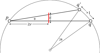
  Figure 4: Proof of Lemma 3.5. The radius of the circle is at least $1/(4\tan^{-1}(\varepsilon/r))$, so edge $pq^{\prime}$ is tense.

  ${\square}$

Lemma 3.6

The relaxed edges inside any slab of constant width are incident to at most $O(r)$ points in $P$.

• Let $\sigma$ be a slab of width $\omega=O(1)$ between two parallel planes, and let $E$ be the set of points in $P$ incident to any relaxed edge contained in $\sigma$. To prove that $\mathopen{|}E\mathclose{|}=O(r)$, we use a variant of our earlier ‘Swiss cheese’ packing argument [52]. Intuitively, we take the intersection of the bounding sphere of $P$ and the slab $\sigma$, remove the Delaunay circumspheres of relaxed edges in $\sigma$, argue that the resulting ‘Swiss cheese slice’ has small surface area, and then charge a constant amount of surface area to each endpoint in $E$. To formalize this argument, we need to slightly expand $\sigma$ and slightly contract the Delaunay balls.

  

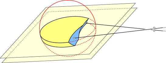
  Figure 5: The Swiss cheese slice $\Sigma$ determined by two relaxed crossing edges intersecting a common pixel. The darker (blue) portion of the surface is $H$. The contracted Delaunay balls $b_{p}$ are not shown.

Let $\sigma^{\prime}$ be a parallel slab with the same central plane as $\sigma$, with slightly larger width $\omega+1$. Let $\bigcirc P$ denote the sphere of radius $r$ containing $P$. Let $D$ be the intersection of $\sigma^{\prime}$ with the sphere of radius $r+1$ concentric with $\bigcirc P$. The volume of $D$ is at most $\pi(\omega+1)(r+1)^{2}=O(r^{2})$.

For each point $p\in E$, we define two balls: $B_{p}$ is the smallest Delaunay ball of some relaxed edge $pq$, and $b_{p}$ is the open ball concentric with $B_{p}$ but with radius smaller by $1/3$. The radius of $B_{p}$ is at most $4r$, and the radius of $b_{r}$ is at most $4r-1/3$.

Finally, we define the ‘Swiss cheese slice’ $\Sigma=D\setminus\bigcup_{p\in E}b_{p}$. For each point $p\in E$, let $h_{p}=\partial\Sigma\cap\partial b_{p}$ be the concave surface of the corresponding ‘hole’ not eaten by any other ball, and let $H=\bigcup_{p\in E}h_{p}$. Equivalently, $H=\partial\Sigma\setminus\partial D$. See Figure 5.

We claim that the surface area of $H$ is only $O(r)$. The proof of this claim is elementary but tedious; we give the proof separately below. By an argument identical to Lemma 2.6 of [52], the ball of unit diameter centered at any point $p\in E$ contains at least $\Omega(1)$ of this surface area—for completeness, we also include this argument below. Since these unit-diameter balls are disjoint, we conclude that $E$ contains at most $O(r)$ points.  ${\square}$

Claim 3.6.1

$\operatorname{area}(H)=O(r)$.

• Let $c_{p}$ be the common center of $B_{p}$ and $b_{p}$, and let $a_{p}$ be the axis line through $c_{p}$ and normal to the planes bounding $\sigma$. For any point $x\in h_{p}$, let $\bar{x}$ be its nearest neighbor on the axis $a_{p}$, and let $H_{p}$ be the union of segments $x\bar{x}$ over all $x\in h_{p}$. See Figure 6 for a two-dimensional example. Finally, let $r_{p}=\min_{x\in h_{p}}\mathopen{|}x\bar{x}\mathclose{|}$.

  The triangle inequality implies that $x\bar{x}$ and $y\bar{y}$ have disjoint interiors whenever $x\neq y$, so

  $$\sum_{p\in E}\operatorname{vol}(H_{p})=\operatorname{vol}\left(\bigcup_{p\in E}H_{p}\right)\leq\operatorname{vol}(D)=O(r^{2}).$$ (1)

  We can bound the volume of each hole $H_{p}$ as follows:

  $$\operatorname{vol}(H_{p}) =\iint_{x\in h_{p}}\!\!\frac{\mathopen{|}x\bar{x}\mathclose{|}\cdot\cos\angle c_{p}x\bar{x}}{2}\,dx^{2}$$

  $$=\iint_{x\in h_{p}}\frac{\mathopen{|}x\bar{x}\mathclose{|}^{2}}{2\mathopen{|}xc_{p}\mathclose{|}}\,dx^{2}$$

  $$=\frac{1}{2\mathopen{|}pc_{p}\mathclose{|}}\,\iint_{x\in h_{p}}\mathopen{|}x\bar{x}\mathclose{|}^{2}\,dx^{2}$$

  $$\geq\frac{1}{12r}\,\iint_{x\in h_{p}}\mathopen{|}x\bar{x}\mathclose{|}^{2}\,dx^{2}$$

  $$\geq\frac{r_{p}^{2}}{12r}\operatorname{area}(h_{p}).$$ (2)

  

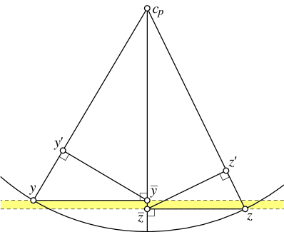
  Figure 6: Proof of Claim 3.6.1. The slab $\sigma^{\prime}$ is shaded.

  The intersection $b_{p}\cap\partial\sigma^{\prime}$ consists of two parallel disks, the smaller of which has radius $r_{p}$. Since both $\sigma^{\prime}$ and the boundary of $B_{p}$ contain the endpoints of some crossing edge $pq$ of length at least $2r$, the larger of these two disks has radius at least $r-\omega-4/3$. Again referring to Figure 6, we choose two points $y,z\in h_{p}\cap\partial\sigma^{\prime}\subseteq b_{p}\cap\partial\sigma^{\prime}$ on the boundary of the larger and smaller disks, respectively, so that $r_{p}=\mathopen{|}z\bar{z}\mathclose{|}$. We can bound this radius as follows:

  $$r_{p}^{2}=\left|z\bar{z}\right|^{2} =\left|zc_{p}\right|^{2}-\left|\bar{z}c_{p}\right|^{2}$$

  $$=\left|zc_{p}\right|^{2}-\left(\left|\bar{z}\bar{y}\right|+\left|\bar{y}c_{p}\right|\right)^{2}$$

  $$=\left|zc_{p}\right|^{2}-\left(\left|\bar{z}\bar{y}\right|+\sqrt{\left|yc_{p}\right|^{2}-\left|y\bar{y}\right|^{2}}\right)^{2}$$

  $$=\left|zc_{p}\right|^{2}-\left(\left|\bar{z}\bar{y}\right|^{2}+2\left|\bar{z}\bar{y}\right|\sqrt{\left|yc_{p}\right|^{2}-\left|y\bar{y}\right|^{2}}+\left|yc_{p}\right|^{2}-\left|y\bar{y}\right|^{2}\right)$$

  $$=\left|y\bar{y}\right|^{2}-2\left|\bar{z}\bar{y}\right|\sqrt{\left|yc_{p}\right|^{2}-\left|y\bar{y}\right|^{2}}-\left|\bar{z}\bar{y}\right|^{2}$$

  $$\geq\left|y\bar{y}\right|^{2}-2\left|\bar{z}\bar{y}\right|\left|yc_{p}\right|-\left|\bar{z}\bar{y}\right|^{2}.$$

  Now substituting the known equations and inequalities

  $$\left|y\bar{y}\right|\geq r-\omega-4/3,\qquad\left|\bar{z}\bar{y}\right|=\omega+1,\qquad\left|yc_{p}\right|<4r-1/3,$$

  we obtain the lower bound

  $$r_{p}^{2}\geq(r-1/3)^{2}-2(\omega+1)(6r-1/3)-(\omega+1)^{2}=\Omega(r^{2}).$$ (3)

  Finally, combining inequalities (1), (2), and (3) yields an upper bound for the surface area of $H$:

  $$\operatorname{area}(H)=\sum_{p\in E}\operatorname{area}(h_{p})\leq\sum_{p\in E}\frac{12r}{r_{p}^{2}}\operatorname{vol}(H_{p})=O(1/r)\cdot\sum_{p\in E}\operatorname{vol}(H_{p})=O(r).$$

  ${\square}$

Claim 3.6.2 (Lemma 2.6 of [52])

Let $U$ be any unit-diameter ball contained in $\Sigma$ whose center is distance $1/3$ from $H$. Then $U$ contains $\Omega(1)$ surface area of $H$.

• 

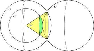
  Figure 7: Proof of Claim 3.6.2.

  Without loss of generality, assume that $U$ is centered at the origin and that $(0,0,1/3)$ is the closest point of $H$ to the origin. Let $U^{\prime}$ be the open ball of radius $1/3$ centered at the origin, let $V$ be the open unit ball centered at $(0,0,5/6)$, and let $W$ be the cone whose apex is the origin and whose base is the circle $\partial U\cap\partial V$. See Figure 7. $U^{\prime}$ lies entirely inside $\Sigma$, and since $r\geq 1$, we easily observe that $V$ lies entirely outside $\Sigma$. Thus, the surface area of $H\cap W\subseteq H\cap U$ is at least the area of the spherical cap $\partial U^{\prime}\cap W$, which is $\pi/27$.  ${\square}$

Together, Lemmas 3.4, 3.5, and 3.6 imply that $O(r)$ relaxed edges intersect any pixel. Since there are $O(r^{2})$ pixels, we conclude that there are $O(r^{3})$ relaxed edges overall.

3.3 Tense Edges Are Easy to Relax

In order to count the tense crossing edges of $P\cup Q$, we will show that there are a constant number of transformations of space, such that every tense edge is mapped to a relaxed edge at least once.

A Möbius transformation is a continuous bijection from the extended Euclidean space $\widehat{\smash{\mathbb{R}^{d}}\vphantom{R}}={\mathbb{R}^{d}\cup\{\infty\}}\simeq\mathbb{S}^{d}$ to itself, such that the image of any sphere is a sphere. (A hyperplane in $\mathbb{R}^{d}$ is a sphere through $\infty$ in $\widehat{\smash{\mathbb{R}^{d}}\vphantom{R}}$.) The space of Möbius transformations is generated by inversions. Examples include reflections (inversions by hyperplanes), translations (the composition of two parallel reflections), dilations (the composition of two concentric inversions), and the well-known stereographic lifting map from $\widehat{\smash{\mathbb{R}^{d}}\vphantom{R}}$ to $\mathbb{S}^{d}\subset\mathbb{R}^{d+1}$ relating $d$-dimensional Delaunay triangulations to ${(d+1)}$-dimensional convex hulls [21]:

$$\lambda(x_{1},x_{2},\dots,x_{d})=\frac{(x_{1},x_{2},\dots,x_{d},1)}{x_{1}^{2}+x_{2}^{2}+\cdots+x_{d}^{2}+1},\qquad\lambda(\infty)=(0,0,\dots,0,0).$$

Möbius transformations are also the maps induced on the boundary of hyperbolic space $\mathbb{S}^{d+1}$ by hyperbolic isometries. Two-dimensional Möbius transformations are also called linear fractional transformations, since they can be written as maps on the extended complex plane $\widehat{\smash{\mathbb{C}}\vphantom{R}}=\mathbb{C}\cup\{\infty\}\simeq\mathbb{S}^{2}$ of the form $z\mapsto{(az+b)/(cz+d)}$ for some complex numbers $a,b,c,d$.

Möbius transformations are conformal, meaning they locally preserve angles. There are infinitely many other two-dimensional conformal maps [85]—in fact, conformal maps are widely used in algorithms for meshing planar domains [38] and parameterizing surfaces [41, 73]—but Möbius transformations are the only conformal maps in dimensions three and higher. Higher-dimensional Möbius transformations are described in detail by Beardon [13]; see also Hilbert and Cohn-Vossen [68], Thurston [95, 94], or Miller et al. [81].

Let $\Sigma$ be a sphere in $\mathbb{R}^{3}$ with finite radius (not passing through the point $\infty$), and let $\pi:\widehat{\smash{\mathbb{R}^{3}}\vphantom{R}}\to\widehat{\smash{\mathbb{R}^{3}}\vphantom{R}}$ be a conformal transformation. If $\pi(\Sigma)$ is also a finite-radius sphere and the point $\pi(\infty)$ lies in the interior of $\Pi(\Sigma)$, we say that $\pi$ everts $\Sigma$.

Let $S$ be a set of points in $\mathbb{R}^{3}\subset\widehat{\smash{\mathbb{R}^{3}}\vphantom{R}}$, and let $p,q,r,s\in S$ be the vertices of a Delaunay simplex with empty circumsphere $\Sigma$. For any conformal transformation $\kappa$, the sphere $\kappa(\Sigma)$ passes through the points $\kappa(p)$, $\kappa(q)$, $\kappa(r)$, and $\kappa(s)$. This sphere either excludes every other point in $\kappa(S)$, contains every other point in $\kappa(S)$, or is a plane with every other point of $\kappa(S)$ on one side. In other words, $\operatorname{conv}\{\kappa(p),\kappa(q),\kappa(r),\kappa(s)\}$ is either a Delaunay simplex, an anti-Delaunay simplex, or a convex hull facet of $\kappa(S)$. Thus, ignoring degenerate cases, the abstract simplicial complex consisting of Delaunay and anti-Delaunay simplices of any point set, which we call its Delaunay polytope, is invariant under conformal transformations.

In this section, we exploit this conformal invariance to count tense crossing edges. The main idea is to find a small collection of conformal maps, such that for any tense edge, at least one of the maps transforms it into a relaxed edge, by shrinking (but not everting) its circumsphere. In order to apply our earlier arguments to count the transformed edges, we consider only conformal maps that map $P\cup Q$ to another well-separated pair of sets with nearly the same spread.

Recall that $P$ and $Q$ lie inside balls of radius $r$ centered at $(0,0,2r)$ and $(0,0,-2r)$, respectively. Call these balls $\bigcirc P$ and $\bigcirc Q$. We call an orientation-preserving conformal map $\kappa$ a rotary map if it preserves these spheres, that is, if $\kappa(\bigcirc P)=\bigcirc P$ and ${\kappa(\bigcirc Q)=\bigcirc Q}$. Rotary maps actually preserve a continuous one-parameter family of spheres centered on the $z$-axis, including the points $p^{*}=(0,0,\sqrt{3}r)$ and $q^{*}=(0,0,-\sqrt{3}r)$ and the plane $z=0$. (In the space of spheres [35, 43], this family is just the line through $\bigcirc P$ and $\bigcirc Q$.) See Figure 8 for a two-dimensional example.

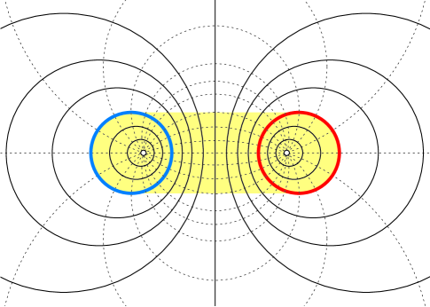
Figure 8: Every rotary map preserves every solid circle and maps every dotted circle to another dotted circle. The bold circles are $\bigcirc P$ and $\bigcirc Q$.

The image of $P\cup Q$ under any rotary map is clearly well-separated. In order to apply our earlier arguments, we also require that these maps do not significantly change the spread.

Lemma 3.7

For any rotary map $\kappa$, the closest pair of points in $\kappa(P\cup Q)$ has distance between $1/3$ and $3$.

• Consider the stereographic lifting map $\lambda:\widehat{\smash{\mathbb{R}^{3}}\vphantom{R}}\to\mathbb{S}^{3}$ that takes $p^{*}$ and $q^{*}$ to opposite poles of $\mathbb{S}^{3}$ and the plane $z=0$ to the equatorial sphere. Any rotary map can be written as $\lambda^{-1}\circ\rho\circ\lambda$, where $\rho$ is a simple rotation about the axis $\lambda(p^{*})\lambda(q^{*})$. (Thus, the space of rotary maps is isomorphic to $SO(3)$, the group of rigid motions of $\mathbb{S}^{2}$.)

  To make the stereographic lifting map $\lambda$ concrete, we embed $\widehat{\smash{\mathbb{R}^{3}}\vphantom{R}}$ and $\mathbb{S}^{3}$ into $\mathbb{R}^{4}$, as the hyperplane $x_{4}=\sqrt{3}r$ and the sphere of radius $\sqrt{3}r/2$ centered at $(0,0,0,\sqrt{3}r/2)$, respectively. Now $\lambda$ is an inversion through the sphere of radius $\sqrt{3}r$ centered at the origin $o=(0,0,0,0)$:

  $$\lambda(x_{1},x_{2},x_{3},x_{4})=\frac{3r^{2}\big{(}x_{1},x_{2},x_{3},x_{4})}{x_{1}^{2}+x_{2}^{2}+x_{3}^{2}+x_{4}^{2}}.\qquad\lambda(\infty)=(0,0,0,0)$$

  Simple calculations (see Beardon [13, pp. 26–27]) imply that for any points $p,q\in\widehat{\smash{\mathbb{R}^{4}}\vphantom{R}}$, we have

  $$\mathopen{|}\lambda(p)\,\lambda(q)\mathclose{|}=\frac{3r^{2}\,\mathopen{|}pq\mathclose{|}}{\mathopen{|}po\mathclose{|}\,\mathopen{|}qo\mathclose{|}}.$$

  The distance from the origin $o$ to any point in $P\cup Q$ (in the hyperplane $w=\sqrt{3}r$) is between $2r$ and $2\sqrt{3}r$. Thus, for any points $p,q\in P\cup Q$, we have

  $$\frac{\mathopen{|}pq\mathclose{|}}{4}\leq\mathopen{|}\lambda(p)\,\lambda(q)\mathclose{|}\leq\frac{3\mathopen{|}pq\mathclose{|}}{4}.$$

  Simple rotations do not change distances at all. Thus, for any rotary map $\pi$, we have

  $$\frac{\mathopen{|}pq\mathclose{|}}{3}\leq\mathopen{|}\pi(p)\,\pi(q)\mathclose{|}\leq 3\mathopen{|}pq\mathclose{|}.$$

  for all points $p,q\in P\cup Q$. The lemma follows immediately.  ${\square}$

Lemma 3.8

There is a set of $O(1)$ rotary maps $\{\pi_{1},\pi_{2},\dots,\pi_{k}\}$ such that any crossing edge of $P\cup Q$ is mapped to a relaxed crossing edge of $\pi_{i}(P\cup Q)$ by some $\pi_{i}$.

• Rotations about the $z$-axis are rotary maps, but since they do not actually change the radius of any sphere, we would like to ignore them. We say that two rotary maps $\kappa_{1}$ and $\kappa_{2}$ are rotationally equivalent if $\kappa_{1}=\rho\circ\kappa_{2}$ for some rotation $\rho$ about the $z$-axis. The rotation class of a rotary map $\kappa$, which we denote $\langle\kappa\rangle$, is the set of maps that are rotationally equivalent to $\kappa$. Since any rotation class $\langle\kappa\rangle$ is uniquely identified by the point $\kappa^{-1}(0,0,0)$ in the $xy$-plane, the space of rotation classes is isomorphic to $\widehat{\smash{\mathbb{R}^{2}}\vphantom{R}}\simeq\mathbb{S}^{2}$.

  Let $B_{1},B_{2},\dots,B_{m}$ be the smallest empty balls containing the crossing edges of $P\cup Q$. For each ball $B_{i}$, let $\kappa_{i}$ denote any rotary map such that $\kappa_{i}(B_{i})$ is centered on the $z$-axis and is not everted, so $\kappa_{i}(B_{i})$ is an empty Delaunay ball of some crossing edge of $\kappa_{i}(P\cup Q)$. We easily observe that $\kappa_{i}(B_{i})$ has radius less than $3r$, so the corresponding crossing edge is relaxed. Thus, for each crossing edge, we have a point $\langle\kappa_{i}\rangle$ on the sphere of rotation classes, corresponding to a rotation class of maps that relax that edge.

  Our key observation is that we have a lot of ‘wiggle room’ in choosing our relaxing maps $\kappa_{i}$. Consider the ball $\bar{B}$ of radius $3r$ centered at the origin; this is the smallest ball containing both $\bigcirc P$ and $\bigcirc Q$. Let $W$ be the set of rotation classes $\langle w\rangle$ such that the radius of $w(\bar{B})$ is at most $4r$ and $w(\bar{B})$ is not everted. $W$ is a circular cap of some constant angular radius $\theta$ on the sphere of rotation classes, centered at $\langle 1\rangle$, the rotation class of the identity map.

  For each $i$, the ball $\kappa_{i}(B_{i})$ lies entirely inside $\bar{B}$, so any rotation class in $W$ transforms $\kappa_{i}(B_{i})$ into another ball of radius at most $4r$. Thus, any rotation class in the set $W_{i}={\left\{\langle w\circ\kappa_{i}\rangle\mid\langle w\rangle\in W\right\}}$ relaxes the $i$th crossing edge. $W_{i}$ is a circular cap of angular radius $\theta$ on the sphere of rotation classes, centered at the point $\langle\kappa_{i}\rangle$.

  

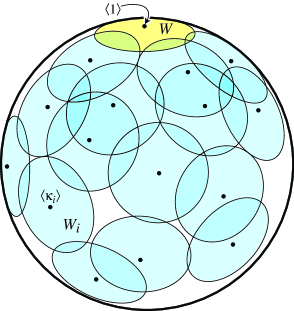
  Figure 9: For each crossing edge, there is a constant-radius cap on the sphere of rotation classes. A constant number of rotation classes stab all these caps.

Since each of these $m$ caps has constant angular radius, we can stab them all with a constant number of points. Specifically, let $\Pi=\{\langle\pi_{1}\rangle,\langle\pi_{2}\rangle,\dots,\langle\pi_{k}\rangle\}\subset\mathbb{S}^{2}$ be a set of $k=O(1/\theta^{2})$ points on the sphere of rotation classes, such that any point in $\mathbb{S}^{2}$ is within angular distance $\theta$ of some point in $\Pi$. (In surface reconstruction terms, $\Pi$ is a $\theta$-sample of the sphere.) Each disk $W_{i}$ contains at least one point in $\Pi$, which implies that each crossing edge is relaxed by some rotation class $\langle\pi_{j}\rangle\in\Pi$. Finally, to satisfy the theorem, we choose an arbitrary rotary map $\pi_{j}$ from each rotation class ${\langle\pi_{j}\rangle\in\Pi}$.  ${\square}$

It follows immediately that $P\cup Q$ has $O(r^{3})$ crossing edges.

3.4 Charging Delaunay Edges to Volume

In the last step of our proof, we count the Delaunay edges in an arbitrary point set $S$ by decomposing it into a collection of subset pairs and counting the crossing edges for each pair.

Let $S$ be an arbitrary set of points with diameter $\Delta$, where the closest pair of points is at unit distance. $S$ is contained in a cube $\square S$ of width $\Delta$. We call an edge of the Delaunay triangulation of $S$ short if its length is less than $5$ and long otherwise. A simple packing argument implies that $S$ has at most $O(\Delta^{3})$ short Delaunay edges.

To count the long Delaunay edges, we construct a well-separated pair decomposition of $S$ [22], based on a simple octtree decomposition of the bounding cube $\square S$. (See Agarwal et al. [2] for a similar decomposition into subset pairs.) Our octtree has $\lceil\log_{2}\Delta\rceil$ levels. At each level $\ell$, there are $8^{\ell}$ cells, each a cube of width $w_{\ell}=\Delta/2^{\ell}$. Our well-separated pair decomposition $\Xi=\left\{(P_{1},Q_{1}),(P_{2},Q_{2}),\dots,(P_{m},Q_{m})\right\}$ contains the points in every pair of cells that are at the same level $\ell$ and are separated by a distance between $3w_{\ell}$ and $6w_{\ell}$.

Every subset pair $(P_{i},Q_{i})\in\Xi$ is well-separated: if the pair is at level $\ell$ in our decomposition, then for some $r_{i}=\Theta(w_{\ell})$, the sets $P_{i}$ and $Q_{i}$ lie in a pair of balls of radius $r_{i}$ separated by distance $2r_{i}$. Thus, by our earlier arguments, the Delaunay triangulation of $P_{i}\cup Q_{i}$ has at most $O(w_{\ell}^{3})$ crossing edges.

For any points $p,q\in S$ such that $\mathopen{|}pq\mathclose{|}\geq 5$, there is a subset pair $(P_{i},Q_{i})\in\Xi$ such that $p\in P_{i}$ and $q\in Q_{i}$. In particular, every long Delaunay edge of $S$ is a crossing edge between some subset pair in $\Xi$. A straightforward counting argument immediately implies that the total number of crossing edges, summed over all subset pairs in $\Xi$, is $O(\Delta^{3}\log\Delta)$ [52]. However, not every crossing edge appears in the Delaunay triangulation of $S$. We remove the final logarithmic factor by charging crossing edges to volume as follows.

Say that a subset pair $(P_{i},Q_{i})\in\Xi$ is relevant if some pair of points $p_{i}\in P_{i}$ and $q_{i}\in Q_{i}$ are Delaunay neighbors in $S$. For each relevant pair $(P_{i},Q_{i})$, we define a large, close, and empty witness ball $B_{i}$ as follows. Choose an arbitrary crossing edge $p_{i}q_{i}$ of $P_{i}\cup Q_{i}$. If $P_{i}$ and $Q_{i}$ are at level $\ell$ in our decomposition, then the distance between $p_{i}$ and $q_{i}$ is at most ${(6+\sqrt{3})w_{\ell}}$. Let $\beta_{i}$ be the smallest ball with $p_{i}$ and $q_{i}$ on its boundary and no point of $S$ in its interior; the radius of $\beta_{i}$ is at least $3w_{\ell}/2$. Let $\beta^{\prime}_{i}$ be a ball concentric with $\beta_{i}$ with radius smaller by $w_{\ell}/2$. Finally, let $B_{i}$ be the ball of radius $w_{\ell}$ inside $\beta^{\prime}_{i}$ whose center is closest to the midpoint of segment $p_{i}q_{i}$. See Figure 10.

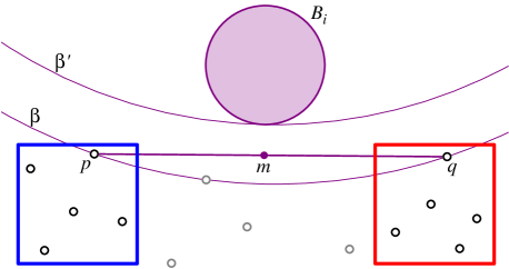
Figure 10: Defining the witness ball $B_{i}$ for a relevant subset pair.

$B_{i}$ is clearly empty. The distance from any point in $B_{i}$ to any point in $S$ is at least $w_{\ell}/2$, since $B_{i}\subset\beta^{\prime}$. On the other hand, the triangle inequality implies that every point in $B_{i}$ has distance less than $(7+\sqrt{3})w_{\ell}/2<4.3661w_{\ell}$ either to $p$ or to $q$, and thus to some cell at level $\ell$ in the octtree. It follows that if two witness balls overlap, their levels differ by at most $\lceil\lg(7+\sqrt{3})\rceil=4$. Moreover, since any ball of radius $(7+\sqrt{3})w_{\ell}/2$ intersects only a constant number of cells at level $\ell$, at most a constant number of level-$\ell$ witness balls overlap at any point.

For any relevant subset pair at level $\ell$, we can charge its $O(w_{\ell}^{3})$ crossing edges to its witness ball, which has volume $\Omega(w_{\ell}^{3})$. Thus, the total number of relevant crossing edges is at most the sum of the volumes of all the witness balls. Since the witness balls have only constant overlap, the sum of their volumes is only a constant factor larger than the volume of their union. Finally, every witness ball fits inside a cube of width $8\Delta$ concentric with $\square S$. It follows that $S$ has at most $O(\Delta^{3})$ long Delaunay edges.

This completes the proof of Theorem 3.1.

4 Extensions and Implications

4.1 Generalizing Spread

Unfortunately, the spread of a set of points is an extremely fragile measure. Adding a single point to a set can arbitrarily increase its spread, either by being too close to another point, or by being far away from all the other points. However, intuitively, adding a few points to a set does not drastically increase the complexity of its Delaunay triangulation. (In fact, adding points can make the Delaunay triangulation considerably simpler [26, 19].) Clearly, our results can tolerate a small number of outliers in the point set—up to $O(\Delta^{3}/n)$, to be precise—but this is not very satisfying.

We can obtain a stronger result by generalizing the notion of spread. For any integer $k$, define the order-$k$ spread of a set $S$ to be the ratio of the diameter of $S$ to the radius of the smallest ball that contains $k$ points of $S$.

Theorem 4.1

The Delaunay triangulation of any set of points in $\mathbb{R}^{3}$ with order-$k$ spread $\Delta_{k}$ has complexity $O(k^{2}\Delta_{k}^{3})$.

• The proof of Theorem 3.1 needs little modification to prove this result; in fact, the only required changes are in the proofs of Lemmas 3.5 and 3.6.

  Let $P$ and $Q$ be two sets of points contained in balls of radius $r$ separated by distance $2r$, where any unit ball contains at most $k$ points. As before, we separate $P$ and $Q$ with a grid of $O(r^{2})$ circular pixels of constant radius $\varepsilon$. Lemma 3.4 applies verbatim.

  A simple modification of the proof of Lemma 3.5 implies that if $\varepsilon<1/16$, then each point of $P$ is the endpoint of at most $k$ relaxed edges through each pixel $\pi$. Specifically, if $p$ is the endpoint of $k+1$ edges $pq_{0}$, $pq_{1},\dots,pq_{k}$ that all intersect $\pi$, then some pair of points $q_{i}$ and $q_{j}$ would be more than distance $1$ apart, which implies that either $pq_{i}$ or $pq_{j}$ is not relaxed. Similarly, since at most $k$ unit-diameter balls overlap at any point, the set of relaxed endpoints $E\subset P$ contains at most $O(kr)$ points; the rest of the proof of Lemma 3.6 in unchanged.

  It follows that at most $O(k^{2}r)$ relaxed edges intersect any pixel, so there are $O(k^{2}r^{3})$ relaxed crossing edges overall. Lemmas 3.7 and 3.8 now imply that there are $O(k^{2}r^{3})$ crossing edges, and the well-separated pair decomposition argument in Section 3.4 completes the proof.  ${\square}$

This generalization immediately implies the following high-probability bound for random points. Surprisingly, this result appears to be new.

Corollary 4.2

Let $S$ be a set of $n$ points generated independently and uniformly in a cube in $\mathbb{R}^{3}$. The Delaunay triangulation of $S$ has complexity $O(n\log n)$ with high probability.

• Let $C$ be a cube of width $(n/\ln n)^{1/3}$. If we generate $S$ uniformly at random inside $C$, the expected number of points in any unit cube inside $C$ is exactly $\ln n$, and Chernoff’s inequality [83] implies that every unit cube inside $C$ contains $O(\log n)$ points with high probability. Thus, with high probability, $\Delta_{k}=O((n/\ln n)^{1/3})$ for some $k=O(\log n)$. The result now follows immediately from Theorem 4.1.  ${\square}$

4.2 Unions of Several Dense Sets

We can also generalize our upper bound to sets that do not have small spread, provided they can be decomposed into few subsets, where each subset has low spread. If all the subsets have the same ‘scale’, the upper bound is almost immediate.

Theorem 4.3

Let $P_{1},P_{2},\dots,P_{k}$ be sets of points in $\mathbb{R}^{3}$, each with closest pair distance at least $1$ and diameter at most $\Delta$. The Delaunay triangulation of $P_{1}\cup P_{2}\cup\cdots\cup P_{k}$ has complexity $O(k^{2}\Delta^{3})$.

• It suffices to consider the case $k=2$; for larger values of $k$, we separately count Delaunay edges for all $\binom{k}{2}$ pairwise unions.

  Let $P$ and $Q$ be two sets, each with closest pair distance at least $1$ and diameter at most $\Delta$. We say that an edge in the Delaunay triangulation off $P\cup Q$ is bichromatic if it joins a point in $P$ to a point in $Q$, and monochromatic otherwise. Theorem 3.1 immediately implies that there are $O(\Delta^{3})$ monochromatic edges.

  If $P$ and $Q$ are well-separated, every bichromatic edge is a crossing edge, so by our earlier analysis, there are $O(\Delta^{3})$ bichromatic edges. Otherwise, we can define a well-separated pair decomposition by building an octtree over the bounding box of $P\cup Q$, which has width at most $4\Delta$, so that every bichromatic edge is a crossing edge for some well-separated subset pair. By charging bichromatic edges to empty witness balls exactly as before, we conclude that the number of bichromatic edges is still $O(\Delta^{3})$.  ${\square}$

This also provides an alternate proof of Theorem 4.1, since any point set whose order-$k$ spread is $\Delta_{k}$ can be partitioned into $O(k)$ subsets satisfying the conditions of the theorem.

With more effort, we can establish a similar upper bound for unions of arbitrary low-spread sets with arbitrarily different scales. As usual, we start by considering the case of two sets contained in disjoint balls. Let $P$ be a set of points with closest pair distance $1$ inside a ball $\bigcirc P$ of radius $r$, and let $Q$ be a set of points with closest pair distance $\delta\gg 1$ inside a ball $\bigcirc Q$ of radius $R$. We say that $P$ and $Q$ are well-separated if the distance between $\bigcirc P$ and $\bigcirc Q$ is at least $r+R$.

First suppose $P$ and $Q$ are well-separated. To analyze the number of crossing edges, we follow precisely the same outline as our earlier proof. After an appropriate rigid motion, $\bigcirc P$ is centered at $(0,0,2r)$ and that $\bigcirc Q$ is centered at $(0,0,-2R)$. We place a grid of $O(r^{2})$ circular pixels of radius $\varepsilon=O(1)$ on the plane $z=0$, so that every crossing edge passes through a pixel. The proof of Lemma 3.4 immediately implies that the crossing edges passing through any pixel lie in a slab of width $O(R/r)$ between two parallel planes.

Say that an crossing edge is relaxed if its endpoints lie on an empty sphere of radius $O(R+r)$. The proof of Lemma 3.5 immediately implies that each point in $Q$ is an endpoint of at most one relaxed edge passing through any pixel. (However, a point in $P$ might be an endpoint of more than one relaxed edge if $R/\delta<r$.) Lemma 3.6 generalizes as follows.

Lemma 4.4

The relaxed edges passing through any pixel $\pi$ are incident to at most $O(R/\delta+R^{2}/r\delta^{2})$ points in $Q$.

• Let $\sigma$ be the slab of width $O(R/r)$ containing the crossing edges through $\pi$, and let $\sigma^{\prime}$ be a parallel slab of width $O(R/r+\delta)$ with the same central plane. We define the ‘Swiss cheese holes’ $H$ exactly as in the proof of Lemma 3.6. For each relaxed endpoint $q\in Q$, let $U_{q}$ be a ball of radius $\delta/2$ centered at $q$; these balls are disjoint. After an appropriate scaling, Claim 3.6.1 implies that the surface area of $H$ is $O((R+r)(R/r+\delta))=O(R^{2}/r+R\delta)$, and Claim 3.6.2 implies that each ball $U_{q}$ contains $\Omega(\delta^{2})$ of this surface area.  ${\square}$

Since there are $O(r^{2})$ pixels, there are $O(r^{2}R/\delta+rR^{2}/\delta^{2})$ relaxed crossing edges between $P$ and $Q$. Lemmas 3.7 and 3.8 hold without modification, so the total number of crossing edges is $O(r^{2}R/\delta+rR^{2}/\delta^{2})$.

Now suppose $P$ and $Q$ are not well-separated. We want to count the crossing edges—Delaunay edges with one endpoint in each set. Let $\square P$ be a cube of width $r$ containing $P$, let $C$ be a concentric cube of width $8r$. Say that a crossing edge is short if both endpoints are in $C$ and long otherwise. Since the spread of $Q\cap C$ is $O(r/\delta)=O(r)$, our earlier well-separated pair decomposition argument implies that there are $O(r^{3})$ short crossing edges.

Let $\square Q$ be a cube of width $R$ containing $Q$. To count the long crossing edges, we construct an octtree over $\square Q$, subdividing any cell that does not lie entirely inside $C$, whose width is greater than $r$, and whose distance to $\square P$ is less than its width plus $r$. See Figure 11. Let $Q_{\ell}$ be the subset of $Q\setminus C$ inside a leaf cell $\ell$. If the width of $\ell$ is $R/2^{i}$, then the spread of $Q_{\ell}$ is at most $R/2^{i}\delta$. If $Q_{\ell}$ is non-empty, then $P$ and $Q_{\ell}$ are well-separated.

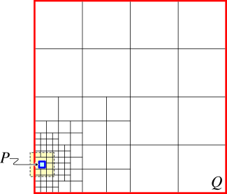
Figure 11: Counting long crossing edges when $P$ and $Q$ are not well-separated.

By our earlier analysis, there are $O(r^{2}R/2^{i}\delta+rR^{2}/4^{i}\delta^{2})$ crossing edges between $P$ and $Q_{\ell}$. Since there are a constant number of leaf cells of any particular width, there are less than

$$\sum_{i=1}^{\infty}O\!\left(\frac{r^{2}R}{2^{i}\delta}+\frac{rR^{2}}{4^{i}\delta^{2}}\right)=O\!\left(\frac{r^{2}R}{\delta}+\frac{rR^{2}}{\delta^{2}}\right)$$

long crossing edges between $P$ and $Q\setminus C$. Thus, the total number of crossing edges is $O(r^{3}+r^{2}R/\delta+rR^{2}/\delta^{2})$.

The spread of $P$ is $O(r)$, and the spread of $Q$ is $O(R/\delta)$. If $r\leq\Delta$ and $R/\delta\leq\Delta$, then our upper bound on the number of crossing edges simplifies to $O(\Delta^{3})$. Theorem 3.1 implies that there are also $O(\Delta^{3})$ non-crossing Delaunay edges, so the overall complexity of the Delaunay triangulation of $P\cup Q$ is $O(\Delta^{3})$.

Generalizing this analysis to more than two sets is straightforward.

Theorem 4.5

Let $P_{1},P_{2},\dots,P_{k}$ be sets of points in $\mathbb{R}^{3}$, each with spread $\Delta$. The Delaunay triangulation of $P_{1}\cup P_{2}\cup\cdots\cup P_{k}$ has complexity $O(k^{2}\Delta^{3})$.

4.3 Regular Triangulations

Regular triangulations are perhaps the most natural generalization of Delaunay triangulations. Let $\hat{p}=(p,r(p))$ denote the ball centered at point $p$ with radius $r(p)$; we can also think of $\hat{p}$ as a point $p$ with an associated weight $r(p)$. Let $\hat{S}$ be a set of balls (or equivalently, a set of weighted points), and let $S$ be the set of centers of balls in $\hat{S}$. The power from a point $x$ to a ball $\hat{p}\in\hat{S}$ is $\mathopen{|}xp\mathclose{|}^{2}-r^{2}(p)$. The power diagram of $\hat{S}$ is the Voronoi diagram with respect to this distance function. The dual of the power diagram is called the regular triangulation of $\hat{S}$. The vertices of this triangulation are all points in $S$; however, some points may not be vertices, as the corresponding region in the power diagram is empty. Regular triangulations can be equivalently defined as the orthogonal (or stereographic) projection of the lower convex hull of a set of points in one higher dimension [44].

The empty circumsphere criterion for Delaunay triangulations generalizes as follows. We say that two balls $\hat{p}$ and $\hat{q}$ are orthogonal if $\mathopen{|}pq\mathclose{|}=r^{2}(p)+r^{2}(q)$, and further than orthogonal if $\mathopen{|}pq\mathclose{|}>r^{2}(p)+r^{2}(q)$. Any sphere that is orthogonal to a set of balls is called an orthosphere of that set. A subset of balls in $\hat{S}$ form a simplex in the regular triangulation of $\hat{S}$ if it has an empty orthosphere, that is, an orthosphere that is further than orthogonal from every other ball in $\hat{S}$.

Theorem 4.6

The regular triangulation of any set of disjoint balls in $\mathbb{R}^{3}$ whose centers have spread $\Delta$ has complexity $O(\Delta^{3})$.

• Let $\hat{S}$ be a set of pairwise-disjoint balls, where the minimum distance between any two centers is $1$, and the maximum distance between any two centers is $\Delta$. Note that the largest ball in $\hat{S}$ has radius less than $\Delta$, which implies that $\hat{S}$ lies inside a ball of radius $2\Delta$.

  Say that an edge $pq$ in the regular triangulation of $\hat{S}$ is local if $\mathopen{|}pq\mathclose{|}<8\min\{r(p),r(q)\}$. We can charge each local edge to whichever endpoint has larger radius. By a straightforward packing argument, each ball $\hat{p}\in\hat{S}$ is charged at most $O(r(p)^{3})$ times. The volume of each ball $\hat{p}$ is $\Omega(r(p)^{3})$. Since the balls are disjoint, the number of local edges bounded by the total volume of the balls, which is $O(\Delta^{3})$.

  To count non-local edges, we follow the same outline as the proof of Theorem 3.1. First consider the well-separated case. Let $\hat{P}$ and $\hat{Q}$ be two sets of balls whose centers lie in balls of radius $r$ separated by distance $2r$. We claim that the regular triangulation of $\hat{P}\cup\hat{Q}$ has $O(r^{3})$ non-local crossing edges. Without loss of generality, we can assume that every ball in $\hat{P}\cup\hat{Q}$ has radius at most $r/4$, since any larger ball has only local crossing edges. Thus, the empty orthospheres of any crossing edge have radius larger than $3r/4$, and the bounding spheres of $\hat{P}$ and $\hat{Q}$ have radius at most $5r/4$ and are separated by distance at least $3r/2$. We modify the proof of Theorem 3.1 by using smallest empty orthospheres instead of empty circumspheres. This replacement increases the constants, but the proofs of most of the lemmas require no other modification. We will describe only the necessary modifications here; refer to the earlier proofs for notation and definitions.

  Edelsbrunner actually proved that regular triangulations have a consistent depth order from any viewpoint [42, 44]. Thus, Lemma 3.3 holds with no modification.

  The proof of Lemma 3.6 requires one qualitative change. First, we shrink each orthosphere $B_{p}$ by only $1/8$ (instead of $1/3$) to obtain $b_{p}$; this does not substantially affect the proof of Claim 3.6.1. We define a new ball $U_{p}$ around each endpoint $p\in E$ as follows. If $r(p)\leq 1/2$, then $U_{p}$ is the unit-diameter ball centered at $p$. Otherwise, $U_{p}$ is any ball of radius $1/4$ inside $\hat{p}$ whose center lies on $B_{p}$; such a ball always exists if $r>10$. A simple modification of the proof of Claim 3.6.2 implies that each ball $U_{p}$ contains $\Omega(1)$ surface area of the Swiss cheese slice $\Sigma$. It follows that $\hat{P}\cup\hat{Q}$ has $O(r^{3})$ relaxed non-local crossing edges.

  The abstract complex consisting of the regular and anti-regular simplices of $\hat{P}\cup\hat{Q}$ is invariant under almost any conformal transformation. We can easily adapt the proof of Lemma 3.7 to show that for any rotary transformation $\pi$, the spread of the centers of $\pi(\hat{P})$ is at most a constant factor larger than the spread of the centers of $\hat{P}$. (Note that the center of the transformed sphere $\pi(\hat{p})$ is not necessarily the image $\pi(p)$ of the original center.) Thus, every rotary image $\pi(\hat{P}\cup\hat{Q})$ has $O(r^{3})$ relaxed non-local crossing edges. Lemma 3.8 requires no modification, so $\hat{P}\cup\hat{Q}$ has $O(r^{3})$ non-local crossing edges.

  Finally, we slightly modify our well-separated pair decomposition argument, by defining a subset pair $(\hat{P}_{i},\hat{Q}_{i})$ to be relevant if and only if it contributes a non-local crossing edge to the regular triangulation. If this is the case, we define $\beta_{i}$ to be the smallest empty orthosphere for any such non-local edge. The remainder of the argument is unchanged. We conclude that the regular triangulation of $\hat{S}$ has $O(\Delta^{3})$ non-local edges.  ${\square}$

We can generalize this upper bound further by allowing the balls to overlap slightly. A set of balls forms a $k$-ply system if no point in space is covered by more than $k$ balls [81]. Applying precisely the same modifications as in the proof of Theorem 4.1, we obtain the following result.

Theorem 4.7

The regular triangulation of any $k$-ply system of balls in $\mathbb{R}^{3}$ whose centers have spread $\Delta$ has complexity $O(k^{2}\Delta^{3})$.

A special case of a $k$-ply system is the hard sphere model commonly used in molecular modeling [77]. A set of balls is hard if the largest and smallest radii differ by a constant factor $r$ and, after shrinking each ball by a constant factor $\rho$, no ball contains the center of any other ball. Halperin and Overmars [66] proved that any hard set of balls forms a $k$-ply system of balls, where $k=O(r^{3}\rho^{3})=O(1)$. (See also Halperin and Shelton [67].)

Corollary 4.8

The regular triangulation of any hard set of balls in $\mathbb{R}^{3}$ whose centers have spread $\Delta$ has complexity $O(\Delta^{3})$.

Combining the ideas in Theorems 4.1, 4.5, and 4.7, we obtain similar bounds for any sets of balls that can be partitioned into a constant number of subsets, each of which is a constant-ply system whose centers have small constant-order spread. We omit further details.

4.4 Surface Data

A somewhat less obvious implication concerns dense surface data. Let $\Sigma$ be a $C^{2}$ surface in $\mathbb{R}^{3}$. Recall from Section 2.2 that a point set $S$ is a uniform $\varepsilon$-sample of $\Sigma$ if, for some constant ${0<\delta<1/2}$, the distance between any surface point $x\in\Sigma$ to the second-closest sample point in $S$ is between $\delta\varepsilon\operatorname{lfs}(x)$ and $\varepsilon\operatorname{lfs}(x)$.

Theorem 4.9

Let $\Sigma$ be a fixed $C^{2}$ surface in $\mathbb{R}^{3}$. The Delaunay triangulation of any uniform $\varepsilon$-sample of $\Sigma$ has complexity $O(n^{3/2})$.

• Let $S$ be a uniform $\varepsilon$-sample of $\Sigma$. This set contains $n=\Theta(\mu/\varepsilon^{2})$ points, where $\mu$ is the sample measure of $\Sigma$ [52, Lemma 3.1]. The spread of $S$ is $\Theta(\Delta/\varepsilon)$, where $\Delta$ is the spread of $\Sigma$, the ratio between the diameter of $\Sigma$ and its minimum local feature size. Thus, by Theorem 3.1, the Delaunay triangulation of $S$ has complexity $O(\Delta^{3}/\varepsilon^{3})=O(n^{3/2}\Delta^{3}/\mu^{3/2})=O(n^{3/2})$.  ${\square}$

This bound is tight in the worst case, for example, when $\Sigma$ is a circular cylinder with spherical caps [52]. Note that Theorem 4.9, which applies to any fixed surface, does not contradict our earlier $\Omega(n^{2}/\log^{2}n)$ lower bound, which requires the surface to depend on $n$ and $\varepsilon$.

Attali and Boissonnat [11] recently showed that under certain sampling conditions, samples of polyhedral surfaces have linear-complexity Delaunay triangulations, improving earlier subquadratic bounds [11]. Unlike most surface-reconstruction results, their sampling conditions do not take local feature size into account (since otherwise samples would be infinite). They define a point set $S$ to be a $(\varepsilon,\kappa)$-sample of $\Sigma$ if the ball of radius $\varepsilon$ centered at any surface point contains at least $1$ and at most $\kappa$ points in $S$; they then show that the Delaunay triangulation of any $(\varepsilon,\kappa)$-sample of a fixed polyhedral surface has complexity $O(n)$.

Theorem 4.10

Let $\Sigma$ be a fixed (not necessarily polyhedral or smooth) surface in $\mathbb{R}^{3}$. The Delaunay triangulation of any $(\varepsilon,\kappa)$-sample of $\Sigma$ has complexity $O(\kappa^{2}n^{3/2})$, where $n$ is the number of sample points.

• Let $S$ be an $(\varepsilon,\kappa)$-sample of $\Sigma$. This set contains $n=\Omega(1/\varepsilon^{2})$ points, where the hidden constant is proportional to the surface area of $\Sigma$. The order-$\kappa$ spread of $S$ is $O(1/\varepsilon)=O(\sqrt{n})$. The result now follows immediately from Theorem 4.1.  ${\square}$

Again, this bound is tight (at least for constant $\kappa$) in the case of a cylinder. Attali and Boissonnat conjecture that for any generic fixed surface, the Delaunay triangulation of any $(\varepsilon,\kappa)$-sample has near-linear complexity; they define a surface to be generic if every medial ball meets the surface in a constant number of points.

Finally, we consider the case of randomly distributed points on surfaces.

Theorem 4.11

Let $\Sigma$ be a fixed surface with surface area $1$, and let $S$ be a set of points generated by a homogeneous Poisson process on $\Sigma$ with rate $n$. With high probability, the Delaunay triangulation of $S$ has complexity $O(n^{3/2}\log^{1/2}n)$.

• let $\sigma$ be a ball of radius $O(\sqrt{(\log n)/n})$ centered on $\Sigma$. The expected number of points in $S\cap\sigma$ is $O(\log n)$, and Chernoff’s inequality [83] implies that $S\cap\sigma$ contains between $1$ and $O(\log n)$ points with high probability. We can cover $\Sigma$ with less than $n$ such balls. Thus, $S$ is an $(\varepsilon,\kappa)$-sample with high probability, where $\varepsilon=O(\sqrt{(\log n)/n})$ and $\kappa=O(\log n)$. The result now follows from Theorem 4.10.  ${\square}$

Unlike most of the other results in this paper, this upper bound is almost certainly not tight. We conjecture that for any fixed piecewise-smooth surface, the Delaunay triangulation of a sufficiently dense uniform random sample has near-linear complexity with high probability. Recent experimental results of Choi and Amenta [30] support this conjecture.

4.5 Algorithms

Finally, our upper bounds immediately imply that several existing algorithms based on Delaunay triangulations are more efficient if the input point set is dense.

Theorem 4.12

The Delaunay triangulation of any set of $n$ points in $\mathbb{R}^{3}$ with spread $\Delta$ can be computed in $O(\Delta^{3}\log n)$ expected time, or in $O(\Delta^{3}\log^{2}n)$ worst-case time.

• To obtain the expected time bound, we apply the standard randomized incremental algorithm of Guibas, Knuth, and Sharir [65], which inserts the points one at a time in random order; see also [48, 34]. The running time of this algorithm can be broken down into a point location and repair phases. In the point location phase, the algorithm locates the Delaunay simplex containing the next point. The total time for all the point location phases is $O(n\log n)$. The repair phase actually inserts the point, repairs the Delaunay triangulation, and updates the point-location data structure. If the newly inserted point has degree $k$ in the updated Delaunay triangulation, then its repair phase costs $O(k)$ time.

  Inserting a point into a set can only increase its spread, by either increasing the diameter, decreasing the closest pair distance, or both. Thus, at all stages of the algorithm, the spread of the points inserted so far is at most $\Delta$, so every intermediate Delaunay triangulation has complexity $O(\Delta^{3})$. It follows that the expected degree of the $i$th inserted point, and thus the time for the $i$th repair phase, is $O(\Delta^{3}/i)$. Therefore, the total time for all repair phases is $\sum_{i=1}^{n}O(\Delta^{3}/i)=O(\Delta^{3}\log n)$. This dominates the total point-location time.

  The worst-case bound follows immediately from the deterministic output-sensitive algorithm of Chan, Snoeyink, and Yap [24].  ${\square}$

Since the Euclidean minimum spanning tree of a set of points is a subcomplex of the Delaunay triangulation, we can also compute it in $O(\Delta^{3}\log n)$ expected time, by first computing the Delaunay triangulation and then running any efficient minimum spanning tree algorithm on its $O(\Delta^{3})$ edges. This immediately improves the $O(n^{4/3+\varepsilon})$-time algorithm of Agarwal et al. [2] whenever $\Delta=O(n^{4/9})$. We can similarly improve the running times for computing other Delaunay substructures, such as Gabriel complexes, $\alpha$-shapes [46], wrap and flow complexes [45, 57, 56, 91], and cocone triangles [9].

Theorem 4.13

Any set of $n$ points in $\mathbb{R}^{3}$ with spread $\Delta$ can be stored in a data structure of size $O(\Delta^{3}\log n)$, so that nearest neighbor queries can be answered in $O(\log^{2}n)$ time.

• We construct a bottom-vertex triangulation of the Voronoi diagram of the points, using a standard randomized incremental algorithm, where the history graph is used as a point-location data structure. A similar algorithm for building (radial triangulations of) two-dimensional Voronoi diagrams is described by Mulmuley [84, Chapter 3.3]. The running time analysis is almost identical to the proof of Theorem 4.12.

  To speed up the search time, we add auxiliary point-location data structures to the history graph. Each insertion destroys several tetrahedra and creates new ones. We cluster the new tetrahedra according to which Voronoi cells contain them. For each cluster, we construct a point-location structure to determine, given a point $q$ inside that cluster, which tetrahedron contains $q$. Because each cluster of tetrahedra shares a common vertex, we can use planar point-location structures with linear size and logarithmic query time [1]. With high probability, the simplex containing any query point $q$ changes $O(\log n)$ times during the incremental construction of the Voronoi diagram. When the simplex containing $q$ changes, we can determine which cluster to query by a simple distance comparison. Thus, the total time to locate $q$ in the final Voronoi diagram is $O(\log^{2}n)$ with high probability. The total space used by the auxiliary structures is bounded by the size of the history graph, which is $O(\Delta^{3}\log n)$ on average. In particular, some ordering of the points gives us a data structure of size $O(\Delta^{3}\log n)$ with worst-case query time $O(\log^{2}n)$.  ${\square}$

5 Denser Regular Triangulations

Despite our success in the previous two sections, our $O(\Delta^{3})$ upper bound does not generalize to arbitrary triangulations, or even arbitrary regular triangulations. Recall that regular triangulations in $\mathbb{R}^{3}$ can be defined as the orthogonal projection of the lower convex hull of a set of points in $\mathbb{R}^{4}$.

Theorem 5.1

For any $n$ and $\Delta<n$, there is a set of $n$ points with spread $\Delta$ with a regular triangulation of complexity $\Omega(n\Delta)$.

• Any affine transformation of $\mathbb{R}^{3}$ lifts to an essentially unique affine transformation of $\mathbb{R}^{d+1}$ that preserves vertical lines and vertical distances. Since affine transformations preserve convexity, it follows that any affine transformation of a regular triangulation is another regular triangulation (but possibly with very different weights). Thus, to prove the theorem, it suffices to construct a set $S$ of $n$ points whose Delaunay triangulation has complexity $\Omega(n\Delta)$, such that some affine image of $S$ has spread $O(\Delta)$.

  Without loss of generality, assume that $\sqrt{n/\Delta}$ is an integer. For each positive integer $i,j\leq\sqrt{n/\Delta}$, let $s(i,j)$ be the line segment with endpoints $(2i,2j,0)\pm((-1)^{i+j},(-1)^{i+j},1)$. Let $S$ be the set of $n$ points containing $\Delta$ evenly spaced points on each segment $s(i,j)$. Straightforward calculations imply that the Delaunay triangulation of $S$ contains at least $\Delta^{2}/4$ edges between any segment $s(i,j)$ and any adjacent segment ${s(i\pm 1,j)}$ or $s(i,j\pm 1)$. Thus, the overall complexity of the Delaunay triangulation of $S$ is $\Omega(n\Delta)$. Applying the linear transformation $f(x,y,z)=(x,y,\Delta z)$ results in a point set $f(S)$ with spread $O(\Delta)$.  ${\square}$

This result does not contradict Theorems 4.6 or 4.7, since the weighted points in our construction are equivalent to balls that overlap heavily. In fact, the largest ball in our construction actually contains the centers of a constant fraction of the other balls.

6 Open Problems

Our results suggest several open problems, the most obvious of which is to simplify our rather complicated proof of Theorem 3.1. The hidden constant in our upper bound is in the millions; the corresponding constant in the lower bound (which seems much closer to the true worst-case complexity) is about $10$.

We conjecture that Theorem 5.1 is tight for arbitrary triangulations. In fact, we believe that any complex of points, edges, and triangles, embedded in $\mathbb{R}^{3}$ so that no triangle crosses an edge, has $O(n\Delta)$ triangles. Even the following special case is still open: What is the minimum spread of a set of $n$ points in $\mathbb{R}^{3}$ in which every pair is joined by a Delaunay edge? We optimistically conjecture that the answer is $n/\pi-o(n)$; this is the spread of $n$ evenly-spaced points on a single turn of a helix with infinitesimal pitch.

What is the worst-case complexity of the convex hull of a set of $n$ points in $\mathbb{R}^{4}$ with spread $\Delta$? Our earlier results [52] already imply a lower bound of $\Omega(\min\{\Delta^{3},n\Delta,n^{2}\})$. This bound is not improved by Theorem 5.1, since our construction requires points with extremely large weights. The only known upper bound is $O(n^{2})$.

Another interesting open problem is to generalize the results in this paper to higher dimensions. Our techniques almost certainly imply an upper bound of $O(\Delta^{d})$ on the number of Delaunay edges, improving our earlier upper bound of $O(\Delta^{d+1})$. Unfortunately, this gives a very weak bound on the overall complexity, which we conjecture to be $O(\Delta^{d})$. What is needed is a technique to directly count $\lfloor d/2\rfloor$-dimensional Delaunay simplices: triangles in $\mathbb{R}^{4}$, tetrahedra in $\mathbb{R}^{6}$, and so on.

Standard range searching techniques can be used to answer nearest neighbor queries in $\mathbb{R}^{3}$ in $O(\log n)$ time using $O(n^{2}/\operatorname{polylog}n)$ space, or in $O(\sqrt{n}\operatorname{polylog}n)$ time using $O(n)$ space [3, 25, 32, 51, 75]. Using these data structures, we can compute the Euclidean spanning tree of a three-dimensional point set in $O(n^{4/3+\varepsilon})$ time [2]. All these results ultimately rely on the simple observation that the Delaunay triangulation of a random sample of a point set is significantly less complex (in expectation) than the Delaunay triangulation of the whole set. Unfortunately, if we try to reanalyze these algorithms in terms of the spread, this argument falls apart—in the worst case, a random sample of a point set with spread $\Delta$ has expected spread close to $\Delta$, so the Delaunay triangulation of the subset is not significantly simpler after all! Can random sampling be integrated with our distance-sensitive bounds? Is there a data structure of size $O(n)$ that supports faster nearest neighbor queries when the spread is, say, $O(\sqrt{n})$?

Acknowledgments.

Once again, I thank Edgar Ramos for suggesting well-separated pair decompositions. Thanks also to Edgar Ramos, Herbert Edelsbrunner, Pat Morin, Sariel Har-Peled, Sheng-Hua Teng, Tamal Dey, and Timothy Chan for helpful discussions; to Pankaj Agarwal and Sariel Har-Peled for comments on an earlier draft of the paper; and to the anonymous SODA reviewers for pointing to the work of Miller et al. [79, 81, 80].

References

- [1] U. Adamy and R. Seidel. On the exact worst case query complexity of planar point location. J. Algorithms 37:189–217, 2000.
- [2] P. K. Agarwal, H. Edelsbrunner, O. Schwarzkopf, and E. Welzl. Euclidean minimum spanning trees and bichromatic closest pairs. Discrete Comput. Geom. 6(5):407–422, 1991.
- [3] P. K. Agarwal and J. Erickson. Geometric range searching and its relatives. Advances in Discrete and Computational Geometry, 1–56, 1999. Contemporary Mathematics 223, American Mathematical Society.
- [4] A. Aggarwal and P. Raghavan. Deferred data structures for the nearest-neighbor problem. Inform. Process. Lett. 40(3):119–122, 1991.
- [5] R. Alexander. Geometric methods in the study of irregularities of distribution. Combinatorica 10(2):115–136, 1990.
- [6] N. Alon, M. Katchalski, and W. R. Pulleyblank. The maximum size of a convex polygon in a restricted set of points in the plane. Discrete Comput. Geom. 4:245–251, 1989.
- [7] N. Amenta and M. Bern. Surface reconstruction by Voronoi filtering. Discrete Comput. Geom. 22(4):481–504, 1999.
- [8] N. Amenta, M. Bern, and M. Kamvysselis. A new Voronoi-based surface reconstruction algorithm. Proc. SIGGRAPH ’98, 415–412, 1998.
- [9] N. Amenta, S. Choi, T. K. Dey, and N. Leekha. A simple algorithm for homeomorphic surface reconstruction. Proc. 16th Annu. ACM Sympos. Comput. Geom., 213–222, 2000.
- [10] N. Amenta, S. Choi, and R. Kolluri. The power crust, unions of balls, and the medial axis transform. Internat. J. Comput. Geom. Appl. 19(2–3):127–153, 2001.
- [11] D. Attali and J.-D. Boissonnat. Complexity of Delaunay triangulations of points on polyhedral surfaces. Rapport de recherche 4015, INRIA Sophia-Antipolis, July 2001. http://www.inria.fr/rrrt/rr-4232.html.
- [12] D. Attali and J.-D. Boissonnat. A linear bound on the complexity of the Delaunay triangulations of points on polyhedral surfaces. Proc. 7th Annu. ACM Sympos. Solid Modeling Appl., 139–146, 2002.
- [13] A. F. Beardon. The Geometry of Discrete Groups. Graduate Texts in Mathematics 91. Springer-Verlag, 1983.
- [14] J. L. Bentley, B. W. Weide, and A. C. Yao. Optimal expected-time algorithms for closest-point problems. ACM Trans. Math. Softw. 6:563–580, 1980.
- [15] M. de Berg. Ray Shooting, Depth Orders and Hidden Surface Removal. Lecture Notes Comput. Sci. 703. Springer-Verlag, Berlin, Germany, 1993.
- [16] M. de Berg, M. J. Katz, A. F. van der Stappen, and J. Vleugels. Realistic input models for geometric algorithms. Proc. 13th Annu. ACM Sympos. Comput. Geom., 294–303, 1997.
- [17] M. de Berg, M. Overmars, and O. Schwarzkopf. Computing and verifying depth orders. SIAM J. Comput. 23:437–446, 1994.
- [18] J. Bernal. On the expected complexity of the 3-dimensional Voronoi diagram. Tech. Rep. NISTIR 4321, National Inst. of Standards and Technology, May 1990. ftp://math.nist.gov/pub/bernal/vor3comp.ps.
- [19] M. Bern, D. Eppstein, and J. Gilbert. Provably good mesh generation. J. Comput. Syst. Sci. 48:384–409, 1994.
- [20] J.-D. Boissonnat and F. Cazals. Smooth surface reconstruction via natural neighbour interpolation of distance functions. Proc. 16th Annu. ACM Sympos. Comput. Geom., 223–232, 2000.
- [21] K. Q. Brown. Voronoi diagrams from convex hulls. Inform. Process. Lett. 9(5):223–228, 1979.
- [22] P. B. Callahan and S. R. Kosaraju. A decomposition of multidimensional point sets with applications to -nearest-neighbors and -body potential fields. J. ACM 42:67–90, 1995.
- [23] D. E. Cardoze and L. Schulman. Pattern matching for spatial point sets. Proc. 39th Annu. IEEE Sympos. Found. Comput. Sci., 156–165, 1998.
- [24] T. M. Chan, J. Snoeyink, and C. K. Yap. Primal dividing and dual pruning: Output-sensitive construction of -d polytopes and -d Voronoi diagrams. Discrete Comput. Geom. 18:433–454, 1997.
- [25] B. Chazelle. Cutting hyperplanes for divide-and-conquer. Discrete Comput. Geom. 9(2):145–158, 1993.
- [26] B. Chazelle, H. Edelsbrunner, L. J. Guibas, J. E. Hershberger, R. Seidel, and M. Sharir. Slimming down by adding; selecting heavily covered points. Proc. 6th Annu. ACM Sympos. Comput. Geom., 116–127, 1990.
- [27] B. Chazelle, H. Edelsbrunner, L. J. Guibas, M. Sharir, and J. Stolfi. Lines in space: Combinatorics and algorithms. Algorithmica 15:428–447, 1996.
- [28] H.-L. Cheng, T. K. Dey, H. Edelsbrunner, and J. Sullivan. Dynamic skin triangulation. Discrete Comput. Geom. 25(4):525–568, 2001.
- [29] S.-W. Cheng, T. K. Dey, H. Edelsbrunner, M. A. Facello, and S.-H. Teng. Sliver exudation. Proc. 15th Annu. Sympos. Comput. Geom., 1–13, 1999.
- [30] S. Choi and N. Amenta. Delaunay triangulation programs on surface data. Proc. 13th Annu. ACM-SIAM Sympos. Discrete Algorithms, 135–136, 2002.
- [31] K. L. Clarkson. A probabilistic algorithm for the post office problem. Proc. 17th Annu. ACM Sympos. Theory Comput., 175–184, 1985.
- [32] K. L. Clarkson. A randomized algorithm for closest-point queries. SIAM J. Comput. 17:830–847, 1988.
- [33] K. L. Clarkson. Nearest neighbor queries in metric spaces. Discrete Comput. Geom. 22:63–93, 1999.
- [34] K. L. Clarkson and P. W. Shor. Applications of random sampling in computational geometry, II. Discrete Comput. Geom. 4:387–421, 1989.
- [35] O. Devillers, S. Meiser, and M. Teillaud. The space of spheres, a geometric tool to unify duality results on Voronoi diagrams. Report 1620, INRIA Sophia-Antipolis, 1992. http://www.inria.fr/rrrt/rr-1620.html.
- [36] A. K. Dewdney and J. K. Vranch. A convex partition of with applications to Crum’s problem and Knuth’s post-office problem. Utilitas Math. 12:193–199, 1977.
- [37] T. K. Dey, S. Funke, and E. A. Ramos. Surface reconstruction in almost linear time under locally uniform sampling. Abstracts 17th European Workshop Comput. Geom., 129–132, 2001. Freie Universität Berlin. http://www.cis.ohio-state.edu/~tamaldey/paper/recon-linear/surf.ps.gz.
- [38] T. A. Driscoll and S. A. Vavasis. Numerical conformal mapping using cross-ratios and Delaunay triangulation. SIAM J. Sci. Comput. 19:1783–1803, 1998.
- [39] R. Dwyer. The expected number of -faces of a Voronoi diagram. Internat. J. Comput. Math. 26(5):13–21, 1993.
- [40] R. A. Dwyer. Higher-dimensional Voronoi diagrams in linear expected time. Discrete Comput. Geom. 6:343–367, 1991.
- [41] M. Eck, T. DeRose, T. Duchamp, H. Hoppe, M. Lounsbery, and W. Stuetzle. Multiresolution analysis of arbitrary meshes. Proc. SIGGRAPH ’95, 173–182, 1995.
- [42] H. Edelsbrunner. An acyclicity theorem for cell complexes in dimensions. Combinatorica 10(3):251–260, 1990.
- [43] H. Edelsbrunner. Deformable smooth surface design. Discrete Comput. Geom. 21:87–115, 1999.
- [44] H. Edelsbrunner. Geometry and Topology for Mesh Generation. Cambridge University Press, Cambridge, England, 2001.
- [45] H. Edelsbrunner. Surface reconstruction by wrapping finite point sets in space. To appear in Discrete & Computational Geometry: The Goodman-Pollack Festschrift, 2003. Algorithms and Combinatorics, Springer-Verlag.
- [46] H. Edelsbrunner, D. G. Kirkpatrick, and R. Seidel. On the shape of a set of points in the plane. IEEE Trans. Inform. Theory IT-29:551–559, 1983.
- [47] H. Edelsbrunner, X.-Y. Li, G. Miller, A. Stathopoulos, D. Talmor, S.-H. Teng, A. Üngör, and N. Walkington. Smoothing and cleaning up slivers. Proc. 32nd Annu. ACM Sympos. Theory Comput., 273–277, 2000.
- [48] H. Edelsbrunner and N. R. Shah. Incremental topological flipping works for regular triangulations. Algorithmica 15:223–241, 1996.
- [49] H. Edelsbrunner, P. Valtr, and E. Welzl. Cutting dense point sets in half. Discrete Comput. Geom. 17:243–255, 1997.
- [50] B. Efron. The problem of the two nearest neighbors (abstract). Ann. Math. Statist. 38:298, 1967.
- [51] J. Erickson. Space-time tradeoffs for emptiness queries. SIAM J. Comput. 29(6):1968–1996, 2000.
- [52] J. Erickson. Nice point sets can have nasty Delaunay triangulations. Proc. 17th Annu. ACM Sympos. Comput. Geom., 96–105, 2001. http://www.cs.uiuc.edu/~jeffe/pubs/spread.html.
- [53] J. Erickson. Dense points sets have sparse Delaunay triangulations. Proc. 13th Annu. ACM-SIAM Sympos. Discrete Algorithms, 125–134, 2002.
- [54] S. Funke and E. A. Ramos. Smooth-surface reconstruction in near-linear time. Proc. 15th Annu. ACM-SIAM Sympos. Discrete Algorithms, pp. 781–790, 2002.
- [55] M. Gavrilov, P. Indyk, R. Motwani, and S. Venkatasubramanian. Geometric pattern matching: A performance study. Proc. 15th Annu. ACM Sympos. Comput. Geom., 79–85, 1999.
- [56] J. Giesen and M. John. A new diagram from disks in the plane. Proc. 19th Annu. Sympos. Theoretical Aspects Comput. Sci., 238–249, 2002. Lecture Notes Comput. Sci. 2285, Springer-Verlag.
- [57] J. Giesen and M. John. The flow complex: A data structure for geometric modeling. To appear in Proc. 14th Annu. ACM-SIAM Sympos. Discrete Algorithms, 2003.
- [58] E. N. Gilbert. Random subdivisions of space into crystals. Ann. Math. Statist. 33:958–972, 1962.
- [59] M. J. Golin and H. S. Na. On the average complexity of 3D-Voronoi diagrams of random points on convex polytopes. Proc. 12th Canad. Conf. Comput. Geom., 127–135, 2000. http://www.cs.unb.ca/conf/cccg/eProceedings/.
- [60] M. J. Golin and H. S. Na. On the average complexity of 3D-Voronoi diagrams of random points on convex polytopes. Tech. Rep. HKUST-TCSC-2001-08, Hong Kong Univ. Sci. Tech., June 2001. http://www.cs.ust.hk/tcsc/RR/2001-08.ps.gz.
- [61] M. J. Golin and H. S. Na. On the proofs of two lemmas describing the intersections of spheres with the boundary of a convex polytope. Tech. Rep. HKUST-TCSC-2001-09, Hong Kong Univ. Sci. Tech., July 2001. http://www.cs.ust.hk/tcsc/RR/2001-09.ps.gz.
- [62] M. J. Golin and H. S. Na. The probabilistic complexity of the Voronoi diagram of points on a polyhedron. Proc. 18th Annu. ACM Sympos. Comput. Geom., 209–216, 2002.
- [63] J. E. Goodman, R. Pollack, and B. Sturmfels. Coordinate representation of order types requires exponential storage. Proc. 21st Annu. ACM Sympos. Theory Comput., 405–410, 1989.
- [64] J. E. Goodman, R. Pollack, and B. Sturmfels. The intrinsic spread of a configuration in . J. Amer. Math. Soc. 3:639–651, 1990.
- [65] L. J. Guibas, D. E. Knuth, and M. Sharir. Randomized incremental construction of Delaunay and Voronoi diagrams. Algorithmica 7:381–413, 1992.
- [66] D. Halperin and M. H. Overmars. Spheres, molecules, and hidden surface removal. Comput. Geom. Theory Appl. 11:83–102, 1998.
- [67] D. Halperin and C. R. Shelton. A perturbation scheme for spherical arrangements with application to molecular modeling. Comput. Geom. Theory Appl. 10:273–287, 1998.
- [68] D. Hilbert and S. Cohn-Vossen. Geometry and the Imagination. Chelsea Publishing Company, New York, NY, 1952.
- [69] H. Hiyoshi and K. Sugihara. Voronoi-based interpolation with higher continuity. Proc. 16th Annu. ACM Sympos. Comput. Geom., 242–250, 2000.
- [70] M. Inaba, N. Katoh, and H. Imai. Applications of weighted Voronoi diagrams and randomization to variance-based -clustering. Proc. 10th Annu. ACM Sympos. Comput. Geom., 332–339, 1994.
- [71] P. Indyk, R. Motwani, and S. Venkatasubramanian. Geometric matching under noise: Combinatorial bounds and algorithms. Proc. 8th Annu. ACM-SIAM Sympos. Discrete Algorithms, 457–465, 1999.
- [72] D. Krznaric and C. Levcopoulos. Computing hierarchies of clusters from the Euclidean minimum spanning tree in linear time. Proc. 15th Conf. Found. Softw. Tech. Theoret. Comput. Sci., 443–455, 1995. Lecture Notes Comput. Sci. 1026, Springer-Verlag.
- [73] A. W. F. Lee, W. Sweldens, P. Schröder, L. Cowsar, and D. Dobkin. MAPS: Multiresolution adaptive parameterization of surfaces. Proc. SIGGRAPH ’98, 95–104, 1998.
- [74] X.-Y. Li and S.-H. Teng. Generating well-shaped Delaunay meshes in 3D. Proc. 12th Annu. ACM-SIAM Sympos. Discrete Algorithms, 28–37, 2001.
- [75] J. Matoušek. Range searching with efficient hierarchical cuttings. Discrete Comput. Geom. 10(2):157–182, 1993.
- [76] J. L. Meijering. Interface area, edge length, and number of vertices in crystal aggregates with random nucleation. Research Report 8, Philips, 1953.
- [77] P. G. Mezey. Molecular surfaces. Reviews in Computational Chemistry, 1990. vol. 1, VCH Publishers.
- [78] R. E. Miles. The random division of space. Adv. Appl. Prob. (Suppl.) 5:243–266, 1972.
- [79] G. L. Miller, D. Talmor, and S.-H. Teng. Optimal coarsening of unstructured meshes. J. Algorithms 31(1):29–65, 1999.
- [80] G. L. Miller, D. Talmor, S.-H. Teng, and N. Walkington. A Delaunay based numerical method for three dimensions: generation, formulation, and partition. Proc. 27th Annu. ACM Sympos. Theory Comput., 683–692, 1995.
- [81] G. L. Miller, S.-H. Teng, W. Thurston, and S. A. Vavasis. Separators for sphere-packings and nearest neighbor graphs. J. ACM 44:1–29, 1997.
- [82] J. Møller. Random tessellations in . Adv. Appl. Prob. 21:37–73, 1989.
- [83] R. Motwani and P. Raghavan. Randomized Algorithms. Cambridge University Press, New York, NY, 1995.
- [84] K. Mulmuley. Computational Geometry: An Introduction Through Randomized Algorithms. Prentice Hall, Englewood Cliffs, NJ, 1993.
- [85] T. Needham. Visual Complex Analysis. Oxford University Press, 1999.
- [86] A. Okabe, B. Boots, K. Sugihara, and S. N. Chiu. Spatial Tessellations: Concepts and Applications of Voronoi Diagrams, second edition. John Wiley & Sons, Chichester, UK, 2000.
- [87] T. Schreiber. A Voronoi diagram based adaptive -means-type clustering algorithm for multidimensional weighted data. Proc. Computational Geometry: Methods, Algorithms and Applications, 265–275, 1991. Lecture Notes Comput. Sci. 553, Springer-Verlag.
- [88] R. Seidel. Constructing higher-dimensional convex hulls at logarithmic cost per face. Proc. 18th Annu. ACM Sympos. Theory Comput., 404–413, 1986.
- [89] M. Sharir, S. Smorodinsky, and G. Tardos. An improved bound for -sets in three dimensions. Proc. 16th Annu. ACM Sympos. Comput. Geom., 43–49, 2000.
- [90] J. R. Shewchuk. Tetrahedral mesh generation by Delaunay refinement. Proc. 14th Annu. ACM Sympos. Comput. Geom., 86–95, 1998.
- [91] D. Siersma. Voronoi diagrams and Morse theory of the distance function. Geometry in Present Day Science, 187–208, 1999. World Scientific.
- [92] D. Talmor. Well-Spaced Points and Numerical Methods. Ph.D. thesis, School of Computer Science, Carnegie Mellon University, Pittsburgh, PA, August 1997. http://reports-archive.adm.cs.cmu.edu/anon/1997/abstracts/97-164.html. Technical report CMU-CS-97-164.
- [93] S.-H. Teng. Points, Spheres, and Separators: A Unified Geometric Approach to Graph Partitioning. Ph.D. thesis, School of Computer Science, Carnegie Mellon University, Pittsburgh, PA, 1992. Technical report CMU-CS-91-184.
- [94] W. Thurston. Three-Dimensional Geometry and Topology, Volume 1. Princeton University Press, New Jersey, 1997.
- [95] W. P. Thurston. The geometry and topology of 3-manifolds. Mathematical Sciences Research Institite, Berkeley, CA, 1997. http://msri.org/publications/books/gt3m/.
- [96] P. Valtr. Convex independent sets and -holes in restricted planar point sets. Discrete Comput. Geom. 7:135–152, 1992.
- [97] P. Valtr. Planar point sets with bounded ratios of distances. Ph.D. thesis, Fachbereich Mathematik, Freie Universität Berlin, Berlin, Germany, 1994.
- [98] P. Valtr. Lines, line-point incidences and crossing families in dense sets. Combinatorica 16:269–294, 1996.
- [99] K. Verbarg. Approximate center points in dense point sets. Inform. Proc. Letters 61(5):271–278, 1997.
- [100] J. Vleugels. On Fatness and Fitness: Realistic Input Models for Geometric Algorithms. Ph.D. thesis, Dept. Comput. Sci., Univ. Utrecht, Utrecht, The Netherlands, 1997.
- [101] Y. Zhou. Shape Sensitive Geometric Complexity. D.Sc. thesis, Department of Computer Science, Washington University, St. Louis, MO, 2000.