Transformation-Based Learning in the Fast Lane

Abstract

Transformation-based learning has been successfully employed to solve many natural language processing problems. It achieves state-of-the-art performance on many natural language processing tasks and does not overtrain easily. However, it does have a serious drawback: the training time is often intorelably long, especially on the large corpora which are often used in NLP. In this paper, we present a novel and realistic method for speeding up the training time of a transformation-based learner without sacrificing performance. The paper compares and contrasts the training time needed and performance achieved by our modified learner with two other systems: a standard transformation-based learner, and the ICA system [Hepple, 2000]. The results of these experiments show that our system is able to achieve a significant improvement in training time while still achieving the same performance as a standard transformation-based learner. This is a valuable contribution to systems and algorithms which utilize transformation-based learning at any part of the execution.

1 Introduction

Much research in natural language processing has gone into the development of rule-based machine learning algorithms. These algorithms are attractive because they often capture the linguistic features of a corpus in a small and concise set of rules.

Transformation-based learning (TBL) [Brill, 1995] is one of the most successful rule-based machine learning algorithms. It is a flexible method which is easily extended to various tasks and domains, and it has been applied to a wide variety of NLP tasks, including part of speech tagging [Brill, 1995], noun phrase chunking [Ramshaw and Marcus, 1999], parsing [Brill, 1996], phrase chunking [Florian et al., 2000], spelling correction [Mangu and Brill, 1997], prepositional phrase attachment [Brill and Resnik, 1994], dialog act tagging [Samuel et al., 1998], segmentation and message understanding [Day et al., 1997]. Furthermore, transformation-based learning achieves state-of-the-art performance on several tasks, and is fairly resistant to overtraining [Ramshaw and Marcus, 1994].

Despite its attractive features as a machine learning algorithm, TBL does have a serious drawback in its lengthy training time, especially on the larger-sized corpora often used in NLP tasks. For example, a well-implemented transformation-based part-of-speech tagger will typically take over 38 hours to finish training on a 1 million word corpus. This disadvantage is further exacerbated when the transformation-based learner is used as the base learner in learning algorithms such as boosting or active learning, both of which require multiple iterations of estimation and application of the base learner. In this paper, we present a novel method which enables a transformation-based learner to reduce its training time dramatically while still retaining all of its learning power. In addition, we will show that our method scales better with training data size.

2 Transformation-based Learning

The central idea of transformation-based learning (TBL) is to learn an ordered list of rules which progressively improve upon the current state of the training set. An initial assignment is made based on simple statistics, and then rules are greedily learned to correct the mistakes, until no net improvement can be made.

The following definitions and notations will be used throughout the paper:

• The sample space is denoted by $\mathcal{S}$;

• $\mathcal{C}$ denotes the set of possible classifications of the samples;

• $C[s]$ denotes the classification associated with a sample $s$, and $T[s]$ denotes the true classification of $s$;

• $p$ will usually denote a predicate defined on $\mathcal{S}$;

• A rule $r$ is defined as a predicate  -  class label pair, $(p,t)$, where $t\in\mathcal{C}$ is called the target of $r$;

• $\mathcal{R}$ denotes the set of all rules;

• If $r=(p,t)$, $p_{r}$ will denote $p$ and $t_{r}$ will denote $t$;

• A rule $r=(p_{r},t_{r})$ applies to a sample $s$ if $p_{r}(s)=true$ and $t_{r}\neq C[s]$; the resulting sample is denoted by $r(s)$.

Using the TBL framework to solve a problem assumes the existence of:

• An initial class assignment. This can be as simple as the most common class label in the training set, or it can be the output of another classifier.

• A set of allowable templates for rules. These templates determine the types of predicates the rules will test; they have the largest impact on the behavior of the system.

• An objective function $f$ for learning. Unlike in many other learning algorithms, the objective function for TBL will directly optimize the evaluation function. A typical example is the difference in performance resulting from applying the rule:

  $$f\left(r\right)=good\left(r\right)-bad\left(r\right)$$

  where

  $$\begin{array}[]{c}good\left(r\right)=\left|\left\{s|C\left[s\right]\neq T\left[s\right]\wedge C\left[r\left(s\right)\right]=T\left[s\right]\right\}\right|\\ bad\left(r\right)=\left|\left\{s|C\left[s\right]=T\left[s\right]\wedge C\left[r\left(s\right)\right]\neq T\left[s\right]\right\}\right|\end{array}$$

Since we are not interested in rules that have a negative objective function value, only the rules that have a positive $good\left(r\right)$ need be examined. This leads to the following approach:

1. Generate the rules (using the rule template set) that correct at least an error (i.e. $good\left(r\right)>0$), by examining all the incorrect samples ($s$ s.t. $C\left[s\right]\neq T\left[s\right]$);

2. Compute the values $bad\left(\cdot\right)$ for each rule $r$ such that $good(r)>f(b)$ , storing at each point in time the rule $b$ that has the highest score; while computing $bad(r)$, skip to the next rule when

   $$f\left(r\right)<f\left(b\right)$$

The system thus learns a list of rules in a greedy fashion, according to the objective function. When no rule that improves the current state of the training set beyond a pre-set threshold can be found, the training phase ends. During the application phase, the evaluation set is initialized with the initial class assignment. The rules are then applied sequentially to the evaluation set in the order they were learned. The final classification is the one attained when all rules have been applied.

2.1 Previous Work

As was described in the introductory section, the long training time of TBL poses a serious problem. Various methods have been investigated towards ameliorating this problem, and the following subsections detail two of the approaches.

2.1.1 The Ramshaw & Marcus Approach

One of the most time-consuming steps in transformation-based learning is the updating step. The iterative nature of the algorithm requires that each newly selected rule be applied to the corpus, and the current state of the corpus updated before the next rule is learned.

Ramshaw & Marcus [Ramshaw and Marcus, 1994] attempted to reduce the training time of the algorithm by making the update process more efficient. Their method requires each rule to store a list of pointers to samples that it applies to, and for each sample to keep a list of pointers to rules that apply to it. Given these two sets of lists, the system can then easily:

1. identify the positions where the best rule applies in the corpus; and

2. update the scores of all the rules which are affected by a state change in the corpus.

These two processes are performed multiple times during the update process, and the modification results in a significant reduction in running time.

The disadvantage of this method consists in the system having an unrealistically high memory requirement. For example, a transformation-based text chunker training upon a modestly-sized corpus of 200,000 words has approximately 2 million rules active at each iteration. The additional memory space required to store the lists of pointers associated with these rules is about 450 MB, which is a rather large requirement to add to a system.

2.1.2 The ICA Approach

The ICA system [Hepple, 2000] aims to reduce the training time by introducing independence assumptions on the training samples that dramatically reduce the training time with the possible downside of sacrificing performance.

To achieve the speedup, the ICA system disallows any interaction between the learned rules, by enforcing the following two assumptions:

• Sample Independence  —  a state change in a sample (e.g. a change in the current part-of-speech tag of a word) does not change the context of surrounding samples. This is certainly the case in tasks such as prepositional phrase attachment, where samples are mutually independent. Even for tasks such as part-of-speech tagging where intuition suggests it does not hold, it may still be a reasonable assumption to make if the rules apply infrequently and sparsely enough.

• Rule Commitment  —  there will be at most one state change per sample. In other words, at most one rule is allowed to apply to each sample. This mode of application is similar to that of a decision list [Rivest, 1987], where an sample is modified by the first rule that applies to it, and not modified again thereafter. In general, this assumption will hold for problems which have high initial accuracy and where state changes are infrequent.

The ICA system was designed and tested on the task of part-of-speech tagging, achieving an impressive reduction in training time while suffering only a small decrease in accuracy. The experiments presented in Section 4 include ICA in the training time and performance comparisons.

2.1.3 Other Approaches

?) proposed a Monte Carlo approach to transformation-based learning, in which only a fraction of the possible rules are randomly selected for estimation at each iteration. The $\mu$-TBL system described in ?) attempts to cut down on training time with a more efficient Prolog implementation and an implementation of “lazy” learning. The application of a transformation-based learning can be considerably sped-up if the rules are compiled in a finite-state transducer, as described in ?).

3 The Algorithm

The approach presented here builds on the same foundation as the one in [Ramshaw and Marcus, 1994]: instead of regenerating the rules each time, they are stored into memory, together with the two values $good\left(r\right)$ and $bad\left(r\right)$.

The following notations will be used throughout this section:

• $G\left(r\right)=\{s\in\mathcal{S}|p_{r}(s)=true\textrm{ and }C[s]\neq t_{r}\textrm{ and }t_{r}=T[s]\}$  —  the samples on which the rule applies and changes them to the correct classification; therefore, $good(r)=|G(r)|$.

• $B\left(r\right)=\{s\in\mathcal{S}|p_{r}(s)=true\textrm{ and }C[s]\neq t_{r}\textrm{ and }C[s]=T[s]\}$  —  the samples on which the rule applies and changes the classification from correct to incorrect; similarly, $bad(r)=|B(r)|$.

Given a newly learned rule $b$ that is to be applied to $\mathcal{S}$, the goal is to identify the rules $r$ for which at least one of the sets $G\left(r\right),B\left(r\right)$ is modified by the application of rule $b$. Obviously, if both sets are not modified when applying rule $b$, then the value of the objective function for rule $r$ remains unchanged.

The presentation is complicated by the fact that, in many NLP tasks, the samples are not independent. For instance, in POS tagging, a sample is dependent on the classification of the preceding and succeeding 2 samples (this assumes that there exists a natural ordering of the samples in $\mathcal{S}$). Let $V\left(s\right)$ denote the “vicinity” of a sample  —  the set of samples on whose classification the sample $s$ might depend on (for consistency, $s\in V(s)$); if samples are independent, then $V\left(s\right)=\left\{s\right\}$.

3.1 Generating the Rules

Let $s$ be a sample on which the best rule $b$ applies (i.e. $\left[b\left(s\right)\right]\neq C\left[s\right]$). We need to identify the rules $r$ that are influenced by the change $s\rightarrow b\left(s\right)$. Let $r$ be such a rule. $f\left(r\right)$ needs to be updated if and only if there exists at least one sample $s^{\prime}$ such that

$$s^{\prime}\in G\left(r\right)\textrm{ and }b\left(s^{\prime}\right)\notin G\left(r\right)\textrm{ or}$$ (1)

$$s^{\prime}\in B\left(r\right)\textrm{ and }b\left(s^{\prime}\right)\notin B\left(r\right)\textrm{ or}$$ (2)

$$s^{\prime}\notin G\left(r\right)\textrm{ and }b\left(s^{\prime}\right)\in G\left(r\right)\textrm{ or}$$ (3)

$$s^{\prime}\notin B\left(r\right)\textrm{ and }b\left(s^{\prime}\right)\in B\left(r\right)\,\,\,\,$$ (4)

Each of the above conditions corresponds to a specific update of the $good\left(r\right)$ or $bad\left(r\right)$ counts. We will discuss how rules which should get their $good$ or $bad$ counts decremented (subcases (1) and (2)) can be generated, the other two being derived in a very similar fashion.

The key observation behind the proposed algorithm is: when investigating the effects of applying the rule $b$ to sample $s$, only samples $s^{\prime}$ in the set $V\left(s\right)$ need to be checked. Any sample $s^{\prime}$ that is not in the set

$$\operatornamewithlimits{\bigcup}_{\left\{s|b\textrm{ changes}\,s\right\}}V\left(s\right)$$

can be ignored since $s^{\prime}=b(s^{\prime})$.

Let $s^{\prime}\in V\left(s\right)$ be a sample in the vicinity of $s$. There are 2 cases to be examined  —  one in which $b$ applies to $s^{\prime}$ and one in which $b$ does not:

Case I: $c\left(s^{\prime}\right)=c\left(b\left(s^{\prime}\right)\right)$ ($b$ does not modify the classification of sample $s^{\prime}$). We note that the condition

$$s^{\prime}\in G\left(r\right)\textrm{ and }b\left(s^{\prime}\right)\notin G\left(r\right)$$

is equivalent to

$$\begin{array}[]{l}p_{r}\left(s^{\prime}\right)=true\,\wedge\,C\left[s^{\prime}\right]\neq t_{r}\,\wedge\\ \,\,\,\,\,t_{r}=T\left[s^{\prime}\right]\,\wedge\,p_{r}\left(b\left(s^{\prime}\right)\right)=false\end{array}$$ (5)

and the formula

$$s^{\prime}\in B\left(r\right)\textrm{ and }b\left(s^{\prime}\right)\notin B\left(r\right)$$

is equivalent to

$$\begin{array}[]{r}p_{r}\left(s^{\prime}\right)=true\wedge C\left[s^{\prime}\right]\neq t_{r}\wedge\\ C\left[s^{\prime}\right]=T\left[s^{\prime}\right]\wedge p_{r}\left(b\left(s^{\prime}\right)\right)=false\end{array}$$ (6)

(for the full details of the derivation, inferred from the definition of $G\left(r\right)$ and $B\left(r\right)$, please refer to ?)).

These formulae offer us a method of generating the rules $r$ which are influenced by the modification $s^{\prime}\rightarrow b\left(s^{\prime}\right)$:

1. Generate all predicates $p$ (using the predicate templates) that are true on the sample $s^{\prime}$.

2. If $C\left[s^{\prime}\right]\neq T\left[s^{\prime}\right]$ then

   1. If $p\left(b\left(s^{\prime}\right)\right)=false$ then decrease $good\left(r\right)$, where $r$ is the rule created with predicate $p$ s.t. target $T\left[s^{\prime}\right]$;

3. Else

   1. If $p\left(b\left(s^{\prime}\right)\right)=false$ then for all the rules $r$ whose predicate is $p$ and $t_{r}\neq C\left[s^{\prime}\right]$ decrease $bad\left(r\right)$;

The algorithm for generating the rules $r$ that need their $good$ counts (formula (3)) or $bad$ counts (formula (4)) increased can be obtained from the formulae (1) (respectively (2)), by switching the states $s^{\prime}$ and $b\left(s^{\prime}\right)$, and making sure to add all the new possible rules that might be generated (only for (3)).

Case II: $C\left[s^{\prime}\right]\neq C\left[b\left(s^{\prime}\right)\right]$ ($b$ does change the classification of sample $s^{\prime}$). In this case, the formula (5) is transformed into:

$$\begin{array}[]{r}p_{r}\left(s^{\prime}\right)=true\textrm{ }\wedge\textrm{ C}\left[s^{\prime}\right]\neq t_{r}\textrm{ }\wedge\textrm{ }t_{r}=T\left[s^{\prime}\right]\textrm{ }\wedge\\ \left(p_{r}\left(b\left(s^{\prime}\right)\right)=false\vee t_{r}=C\left[b\left(s^{\prime}\right)\right]\right)\end{array}$$ (7)

(again, the full derivation is presented in ?)). The case of (2), however, is much simpler. It is easy to notice that $C\left[s^{\prime}\right]\neq C\left[b\left(s^{\prime}\right)\right]$ and $s^{\prime}\in B\left(r\right)$ implies that $b\left(s^{\prime}\right)\notin B\left(r\right)$; indeed, a necessary condition for a sample $s^{\prime}$ to be in a set $B\left(r\right)$ is that $s^{\prime}$ is classified correctly, $C\left[s^{\prime}\right]=T\left[s^{\prime}\right]$. Since $T\left[s^{\prime}\right]\neq C\left[b\left(s^{\prime}\right)\right]$, results $C\left[b\left(s^{\prime}\right)\right]\neq T\left[s^{\prime}\right]$ and therefore $b\left(s^{\prime}\right)\notin B\left(r\right)$. Condition (2) is, therefore, equivalent to

$$p_{r}\left(s^{\prime}\right)=true\textrm{ }\wedge\textrm{ C}\left[s^{\prime}\right]\neq t_{r}\textrm{ }\wedge\textrm{ C}\left[s^{\prime}\right]=T\left[s^{\prime}\right]$$ (8)

The algorithm is modified by replacing the test $p\left(b\left(s^{\prime}\right)\right)=false$ with the test $p_{r}\left(b\left(s^{\prime}\right)\right)=false\vee C\left[b\left(s\right)\right]=t_{r}$ in formula (1) and removing the test altogether for case of (2). The formulae used to generate rules $r$ that might have their counts increased (equations (3) and (4)) are obtained in the same fashion as in Case I.

3.2 The Full Picture

For all samples $s$ that satisfy $C\left[s\right]\neq T\left[s\right]$, generate all rules $r$ that correct the classification of $s$; increase $good\left(r\right)$. For all samples $s$ that satisfy $C\left[s\right]=T\left[s\right]$ generate all predicates $p$ s.t. $p\left(s\right)=true$; for each rule $r$ s.t. $p_{r}=p$ and $t_{r}\neq C\left[s\right]$ increase $bad\left(r\right)$. 1: Find the rule $b=\arg\max_{r\in\mathcal{R}}f\left(r\right)$. If ($f\left(b\right)<\textrm{Threshold}$ or corpus learned to completion) then quit. For each predicate $p$, let $\mathcal{R}\left(p\right)$ be the rules whose predicate is $p$ ($p_{r}=r$). For each samples $s,s^{\prime}$ s.t. $C\left[s\right]\neq C\left[b\left(s\right)\right]$ and $s^{\prime}\in V\left(s\right)$: If $C\left[s^{\prime}\right]=C\left[b\left(s^{\prime}\right)\right]$ then • for each predicate $p$ s.t. $p\left(s^{\prime}\right)=true$ – If $C\left[s^{\prime}\right]\neq T\left[s^{\prime}\right]$ then * If $p\left(b\left(s^{\prime}\right)\right)=false$ then decrease $good\left(r\right)$, where $r=\left[p,T\left[s^{\prime}\right]\right]$, the rule created with predicate $p$ and target $T\left[s^{\prime}\right]$; – Else * If $p\left(b\left(s^{\prime}\right)\right)=false$ then for all the rules $r\in\mathcal{R}\left(p\right)$ s.t. $t_{r}\neq C\left[s^{\prime}\right]$ decrease $bad\left(r\right)$; • for each predicate $p$ s.t. $p\left(b\left(s^{\prime}\right)\right)=true$ – If $C\left[b\left(s^{\prime}\right)\right]\neq T\left[s^{\prime}\right]$ then * If $p\left(s^{\prime}\right)=false$ then increase $good\left(r\right)$, where $r=\left[p,T\left[s^{\prime}\right]\right]$; – Else * If $p\left(s^{\prime}\right)=false$ then for all rules $r\in\mathcal{R}\left(p\right)$ s.t. $t_{r}\neq C\left[b\left(s^{\prime}\right)\right]$ increase $bad\left(r\right)$; Else • for each predicate $p$ s.t. $p\left(s^{\prime}\right)=true$ – If $C\left[s^{\prime}\right]\neq T\left[s^{\prime}\right]$ then * If $p\left(b\left(s^{\prime}\right)\right)=false\vee C\left[b\left(s^{\prime}\right)\right]=t_{r}$ then decrease $good\left(r\right)$, where $r=\left[p,T\left[s^{\prime}\right]\right]$; – Else * For all the rules $r\in\mathcal{R}$$\left(p\right)$ s.t. $t_{r}\neq C\left[s^{\prime}\right]$ decrease $bad\left(r\right)$; • for each predicate $p$ s.t. $p\left(b\left(s^{\prime}\right)\right)=true$ – If $C\left[b\left(s^{\prime}\right)\right]\neq T\left[s^{\prime}\right]$ then * If $p\left(s^{\prime}\right)=false\vee C\left[s^{\prime}\right]=t_{r}$ then increase $good\left(r\right)$, where $r=\left[p,T\left[s^{\prime}\right]\right]$; – Else * For all rules $r\in\mathcal{R}\left(p\right)$ s.t. $t_{r}\neq C\left[b\left(s^{\prime}\right)\right]$ increase $bad\left(r\right)$; Repeat from step 1:

Figure 1: FastTBL Algorithm

At every point in the algorithm, we assumed that all the rules that have at least some positive outcome ($good\left(r\right)>0$) are stored, and their score computed. Therefore, at the beginning of the algorithm, all the rules that correct at least one wrong classification need to be generated. The bad counts for these rules are then computed by generation as well: in every position that has the correct classification, the rules that change the classification are generated, as in Case 4, and their bad counts are incremented. The entire FastTBL algorithm is presented in Figure 1. Note that, when the bad counts are computed, only rules that already have positive good counts are selected for evaluation. This prevents the generation of useless rules and saves computational time.

The number of examined rules is kept close to the minimum. Because of the way the rules are generated, most of them need to modify either one of their counts. Some additional space (besides the one needed to represent the rules) is necessary for representing the rules in a predicate hash  —  in order to have a straightforward access to all rules that have a given predicate; this amount is considerably smaller than the one used to represent the rules. For example, in the case of text chunking task described in section 4, only approximately 30Mb additional memory is required, while the approach of ?) would require approximately 450Mb.

3.3 Behavior of the Algorithm

As mentioned before, the original algorithm has a number of deficiencies that cause it to run slowly. Among them is the drastic slowdown in rule learning as the scores of the rules decrease. When the best rule has a high score, which places it outside the tail of the score distribution, the rules in the tail will be skipped when the bad counts are calculated, since their good counts are small enough to cause them to be discarded. However, when the best rule is in the tail, many other rules with similar scores can no longer be discarded and their bad counts need to be computed, leading to a progressively longer running time per iteration.

Our algorithm does not suffer from the same problem, because the counts are updated (rather than recomputed) at each iteration, and only for the samples that were affected by the application of the latest rule learned. Since the number of affected samples decreases as learning progresses, our algorithm actually speeds up considerably towards the end of the training phase. Considering that the number of low-score rules is a considerably higher than the number of high-score rules, this leads to a dramatic reduction in the overall running time.

This has repercussions on the scalability of the algorithm relative to training data size. Since enlarging the training data size results in a longer score distribution tail, our algorithm is expected to achieve an even more substantial relative running time improvement over the original algorithm. Section 4 presents experimental results that validate the superior scalability of the FastTBL algorithm.

4 Experiments

Since the goal of this paper is to compare and contrast system training time and performance, extra measures were taken to ensure fairness in the comparisons. To minimize implementation differences, all the code was written in C++ and classes were shared among the systems whenever possible. For each task, the same training set was provided to each system, and the set of possible rule templates was kept the same. Furthermore, extra care was taken to run all comparable experiments on the same machine and under the same memory and processor load conditions.

To provide a broad comparison between the systems, three NLP tasks with different properties were chosen as the experimental domains. The first task, part-of-speech tagging, is one where the commitment assumption seems intuitively valid and the samples are not independent. The second task, prepositional phrase attachment, has examples which are independent from each other. The last task is text chunking, where both independence and commitment assumptions do not seem to be valid. A more detailed description of each task, data and the system parameters are presented in the following subsections.

Four algorithms are compared during the following experiments:

• The regular TBL, as described in section 2;

• An improved version of TBL, which makes extensive use of indexes to speed up the rules’ update;

• The FastTBL algorithm;

• The ICA algorithm [Hepple, 2000].

4.1 Part-of-Speech Tagging

	Brill’s tagger	Regular TBL	Indexed TBL	FastTBL	ICA (Hepple)
Accuracy	$96.61\%$	$96.61\%$	$96.61\%$	$96.61\%$	$96.23\%$
Running time	5879 mins, 46 secs	2286 mins, 21 secs	420 mins, 7 secs	17 mins, 21 secs	6 mins, 13 secs
Time ratio	$0.4$	$1.0$	$5.4$	$131.7$	$367.8$

Table 1: POS tagging: Evaluation and Running Times

The goal of this task is to assign to each word in the given sentence a tag corresponding to its part of speech. A multitude of approaches have been proposed to solve this problem, including transformation-based learning, Maximum Entropy models, Hidden Markov models and memory-based approaches.

The data used in the experiment was selected from the Penn Treebank Wall Street Journal, and is the same used by ?). The training set contained approximately 1M words and the test set approximately 200k words.

Table 1 presents the results of the experiment. All the algorithms were trained until a rule with a score of 2 was reached. The FastTBL algorithm performs very similarly to the regular TBL, while running in an order of magnitude faster. The two assumptions made by the ICA algorithm result in considerably less training time, but the performance is also degraded (the difference in performance is statistically significant, as determined by a signed test, at a significance level of $0.001$). Also present in Table 1 are the results of training Brill’s tagger on the same data. The results of this tagger are presented to provide a performance comparison with a widely used tagger. Also worth mentioning is that the tagger achieved an accuracy of $96.76\%$ when trained on the entire data; a Maximum Entropy tagger [Ratnaparkhi, 1996] achieves $96.83\%$ accuracy with the same training data/test data.

4.2 Prepositional Phrase Attachment

	Regular TBL	Indexed TBL	Fast TBL	ICA (Hepple)
Accuracy	$81.0\%$	$81.0\%$	$81.0\%$	$77.8\%$
Running time	190 mins, 19 secs	65 mins, 50 secs	14 mins, 38 secs	4 mins, 1 sec
Time Ratio	$1.0$	$2.9$	$13$	$47.4$

Table 2: PP Attachment:Evaluation and Running Times

Prepositional phrase attachment is the task of deciding the point of attachment for a given prepositional phrase (PP). As an example, consider the following two sentences:

1. I washed the shirt with soap and water.

2. I washed the shirt with pockets.

In Sentence 1, the PP “with soap and water” describes the act of washing the shirt. In Sentence 2, however, the PP “with pockets” is a description for the shirt that was washed.

Most previous work has concentrated on situations which are of the form VP NP1 P NP2. The problem is cast as a classification task, and the sentence is reduced to a 4-tuple containing the preposition and the non-inflected base forms of the head words of the verb phrase VP and the two noun phrases NP1 and NP2. For example, the tuple corresponding to the two above sentences would be:

1. wash shirt with soap

2. wash shirt with pocket

Many approaches to solving this this problem have been proposed, most of them using standard machine learning techniques, including transformation-based learning, decision trees, maximum entropy and backoff estimation. The transformation-based learning system was originally developed by ?).

The data used in the experiment consists of approximately 13,000 quadruples (VP NP1 P NP2) extracted from Penn Treebank parses. The set is split into a test set of 500 samples and a training set of 12,500 samples. The templates used to generate rules are similar to the ones used by ?) and some include WordNet features. All the systems were trained until no more rules could be learned.

Table 2 shows the results of the experiments. Again, the ICA algorithm learns the rules very fast, but has a slightly lower performance than the other two TBL systems. Since the samples are inherently independent, there is no performance loss because of the independence assumption; therefore the performance penalty has to come from the commitment assumption. The Fast TBL algorithm runs, again, in a order of magnitude faster than the original TBL while preserving the performance; the time ratio is only 13 in this case due to the small training size (only 13000 samples).

4.3 Text Chunking

	Regular TBL	Indexed TBL	Fast TBL	ICA (Hepple)
F-measure	92.30	92.30	92.30	86.20
Running Time	19211 mins, 40 secs	2056 mins, 4secs	137 mins, 57 secs	12 mins, 40 secs
Time Ratio	$1.0$	$9.3$	$139.2$	$1516.7$

Table 3: Text Chunking: Evaluation and Running Times

Text chunking is a subproblem of syntactic parsing, or sentence diagramming. Syntactic parsing attempts to construct a parse tree from a sentence by identifying all phrasal constituents and their attachment points. Text chunking simplifies the task by dividing the sentence into non-overlapping phrases, where each word belongs to the lowest phrasal constituent that dominates it. The following example shows a sentence with text chunks and part-of-speech tags:

[NP A.P._NNP Green_NNP ] [ADVP currently_RB ] [VP has ] [NP 2,664,098_CD shares_NNS] [ADJP outstanding_JJ ] .

The problem can be transformed into a classification task. Following Ramshaw & Marcus’ [Ramshaw and Marcus, 1999] work in base noun phrase chunking, each word is assigned a chunk tag corresponding to the phrase to which it belongs . The following table shows the above sentence with the assigned chunk tags:

Word	POS tag	Chunk Tag
A.P.	NNP	B-NP
Green	NNP	I-NP
currently	RB	B-ADVP
has	VBZ	B-VP
2,664,098	CD	B-NP
shares	NNS	I-NP
outstanding	JJ	B-ADJP
.	.	O

The data used in this experiment is the CoNLL-2000 phrase chunking corpus [Tjong Kim Sang and Buchholz, 2000]. The training corpus consists of sections 15-18 of the Penn Treebank [Marcus et al., 1993]; section 20 was used as the test set. The chunk tags are derived from the parse tree constituents, and the part-of-speech tags were generated by Brill’s tagger [Brill, 1995]. All the systems are trained to completion (until all the rules are learned).

Table 3 shows the results of the text chunking experiments. The performance of the FastTBL algorithm is the same as of regular TBL’s, and runs in an order of magnitude faster. The ICA algorithm again runs considerably faster, but at a cost of a significant performance hit. There are at least 2 reasons that contribute to this behavior:

1. The initial state has a lower performance than the one in tagging; therefore the independence assumption might not hold. 25% of the samples are changed by at least one rule, as opposed to POS tagging, where only 2.5% of the samples are changed by a rule.

2. The commitment assumption might also not hold. For this task, 20% of the samples that were modified by a rule are also changed again by another one.

4.4 Training Data Size Scalability

(a) Running Time versus Training Data Size

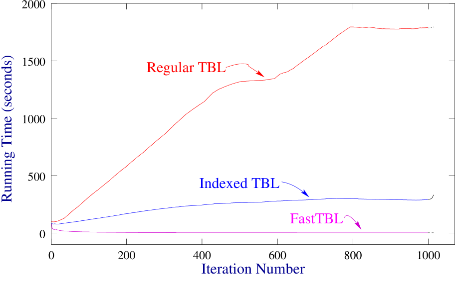
(b) Running Time versus Iteration Number

Figure 2: Algorithm Scalability

A question usually asked about a machine learning algorithm is how well it adapts to larger amounts of training data. Since the performance of the Fast TBL algorithm is identical to that of regular TBL, the issue of interest is the dependency between the running time of the algorithm and the amount of training data.

The experiment was performed with the part-of-speech data set. The four algorithms were trained on training sets of different sizes; training times were recorded and averaged over 4 trials. The results are presented in Figure 2(a). It is obvious that the Fast TBL algorithm is much more scalable than the regular TBL  —  displaying a linear dependency on the amount of training data, while the regular TBL has an almost quadratic dependency. The explanation for this behavior has been given in Section 3.3.

Figure 2(b) shows the time spent at each iteration versus the iteration number, for the original TBL and fast TBL systems. It can be observed that the time taken per iteration increases dramatically with the iteration number for the regular TBL, while for the FastTBL, the situation is reversed. The consequence is that, once a certain threshold has been reached, the incremental time needed to train the FastTBL system to completion is negligible.

5 Conclusions

We have presented in this paper a new and improved method of computing the objective function for transformation-based learning. This method allows a transformation-based algorithm to train an observed 13 to 139 times faster than the original one, while preserving the final performance of the algorithm. The method was tested in three different domains, each one having different characteristics: part-of-speech tagging, prepositional phrase attachment and text chunking. The results obtained indicate that the algorithmic improvement generated by our method is not linked to a particular task, but extends to any classification task where transformation-based learning can be applied. Furthermore, our algorithm scales better with training data size; therefore the relative speed-up obtained will increase when more samples are available for training, making the procedure a good candidate for large corpora tasks.

The increased speed of the Fast TBL algorithm also enables its usage in higher level machine learning algorithms, such as adaptive boosting, model combination and active learning. Recent work [Florian et al., 2000] has shown how a TBL framework can be adapted to generate confidences on the output, and our algorithm is compatible with that framework. The stability, resistance to overtraining, the existence of probability estimates and, now, reasonable speed make TBL an excellent candidate for solving classification tasks in general.

6 Acknowledgements

The authors would like to thank David Yarowsky for his advice and guidance, Eric Brill and John C. Henderson for discussions on the initial ideas of the material presented in the paper, and the anonymous reviewers for useful suggestions, observations and connections with other published material. The work presented here was supported by NSF grants IRI-9502312 and IRI-9618874.

References

- Brill and Resnik, 1994 E. Brill and P. Resnik. 1994. A rule-based approach to prepositional phrase attachment disambiguation. In Proceedings of the Fifteenth International Conference on Computational Linguistics (COLING-1994), pages 1198–1204, Kyoto.
- Brill and Wu, 1998 E. Brill and J. Wu. 1998. Classifier combination for improved lexical disambiguation. Proceedings of COLING-ACL’98, pages 191–195, August.
- Brill, 1995 E. Brill. 1995. Transformation-based error-driven learning and natural language processing: A case study in part of speech tagging. Computational Linguistics, 21(4):543–565.
- Brill, 1996 E. Brill, 1996. Recent Advances in Parsing Technology, chapter Learning to Parse with Transformations. Kluwer.
- Day et al., 1997 D. Day, J. Aberdeen, L. Hirschman, R. Kozierok, P. Robinson, and M. Vilain. 1997. Mixed-initiative development of language processing systems. In Fifth Conference on Applied Natural Language Processing, pages 348–355. Association for Computational Linguistics, March.
- Florian and Ngai, 2001 R. Florian and G. Ngai. 2001. Transformation-based learning in the fast lane. Technical report, Johns Hopkins University, Computer Science Department.
- Florian et al., 2000 R. Florian, J.C. Henderson, and G. Ngai. 2000. Coaxing confidence from an old friend: Probabilistic classifications from transformation rule lists. In Proceedings of SIGDAT-EMNLP 2000, pages 26–34, Hong Kong, October.
- Hepple, 2000 M. Hepple. 2000. Independence and commitment: Assumptions for rapid training and execution of rule-based pos taggers. In Proceedings of the 38th Annual Meeting of the ACL, pages 278–285, Hong Kong, October.
- Lager, 1999 T. Lager. 1999. The -tbl system: Logic programming tools for transformation-based learning. In Proceedings of the 3rd International Workshop on Computational Natural Language Learning, Bergen.
- Mangu and Brill, 1997 L. Mangu and E. Brill. 1997. Automatic rule acquisition for spelling correction. In Proceedings of the Fourteenth International Conference on Machine Learning, pages 734–741, Nashville, Tennessee.
- Marcus et al., 1993 M. P. Marcus, B. Santorini, and M. A. Marcinkiewicz. 1993. Building a large annotated corpus of english: The Penn Treebank. Computational Linguistics, 19(2):313–330.
- Ramshaw and Marcus, 1994 L. Ramshaw and M. Marcus. 1994. Exploring the statistical derivation of transformational rule sequences for part-of-speech tagging. In The Balancing Act: Proceedings of the ACL Workshop on Combining Symbolic and Statistical Approaches to Language, pages 128–135, New Mexico State University, July.
- Ramshaw and Marcus, 1999 L. Ramshaw and M. Marcus, 1999. Natural Language Processing Using Very Large Corpora, chapter Text Chunking Using Transformation-based Learning, pages 157–176. Kluwer.
- Ratnaparkhi, 1996 A. Ratnaparkhi. 1996. A maximum entropy part-of-speech tagger. In Proceedings of the First Conference on Empirical Methods in NLP, pages 133–142, Philadelphia, PA.
- Rivest, 1987 R. Rivest. 1987. Learning decision lists. Machine Learning, 2(3):229–246.
- Roche and Schabes, 1995 E. Roche and Y. Schabes. 1995. Computational linguistics. Deterministic Part of Speech Tagging with Finite State Transducers, 21(2):227–253.
- Samuel et al., 1998 K. Samuel, S. Carberry, and K. Vijay-Shanker. 1998. Dialogue act tagging with transformation-based learning. In Proceedings of the 17th International Conference on Computational Linguistics and the 36th Annual Meeting of the Association for Computational Linguistics, pages 1150–1156, Montreal, Quebec, Canada.
- Samuel, 1998 K. Samuel. 1998. Lazy transformation-based learning. In Proceedings of the 11th Interational Florida AI Research Symposium Conference, pages 235–239, Florida, USA.
- Tjong Kim Sang and Buchholz, 2000 E. Tjong Kim Sang and S. Buchholz. 2000. Introduction to the conll-2000 shared task: Chunking. In Proceedings of CoNLL-2000 and LLL-2000, pages 127–132, Lisbon, Portugal.