From Néel to NPC: Colouring Small Worlds

Abstract

In this note, we present results for the colouring problem on small world graphs created by rewiring square, triangular, and two kinds of cubic (with coordination numbers 5 and 6) lattices. As the rewiring parameter $p$ tends to 1, we find the expected crossover to the behaviour of random graphs with corresponding connectivity. However, for the cubic lattices there is a region near $p=0$ for which the graphs are colourable. This could in principle be used as an additional heuristic for solving real world colouring or scheduling problems. Small worlds with connectivity 5 and $p\sim 0.1$ provide an interesting ensemble of graphs whose colourability is hard to determine. For square lattices, we get good data collapse plotting the fraction of colourable graphs against the rescaled parameter parameter $pN^{-\nu}$ with $\nu=1.35$. No such collapse can be obtained for the data from lattices with coordination number 5 or 6.

Several NP-complete papadimitriou constraint satisfaction problems have recently been found to show threshold phenomena. As some parameter is varied, the fraction of problems than can be solved suddenly changes from 1 to 0 (e.g., cheesemankanefskytaylor ; hogghubermanwilliams ). A related transition occurs for the difficulty of determining whether a problem instance is solvable. Far from the transition, this is almost always easy, while computationally hard problems are clustered near the critical value of the parameter. These transitions have been compared to phase transition appearing in physical systems, and has attracted much interest from physicists who have used techniques from statistical physics such as finite-size scaling kirkpatrickselman and replica symmetry breaking monassonzecchina to study it. Most of the work by physicists has so far been concentrated on the boolean satisfiability problem, though it should be noted that there has been much analytical work on the number partitioning problem mertens .

One important NP-complete problem is the k-colouring problem (k-col). It consists of colouring all the nodes of a graph using k colours in such a way that no edge joins two nodes of the same colour. This problem is particularly interesting for physicists, since it corresponds to finding the zero temperature ground state of an antiferromagnetic k-state Potts model. Graph colouring also has many real-world applications, including scheduling and register-allocation problems. For the k-col problem on random graphs with average degree $\gamma$, Achlioptas and Friedgut achlioptasfriedgut have shown rigorously that there is a $\gamma_{c}$ where the fraction of colourable graphs jumps from 1 to 0. Even though there is currently no exact analytical result for the value of $\gamma_{c}$, Achlioptas achlioptas:thesis has bound it rigorously by $3.84<\gamma_{c}<5.05$.

Small world graphs have recently been introduced in an attempt to capture the topological properties of real graphs. Regular lattices have long average distance between nodes, but show a high degree of clustering (i.e., if we remove a node from the graph, its neighbours will still have short paths between them). On the other hand, random graphs bollobas have no clustering and small average distances. Watts and Strogatz wattsstrogatz:nature ; wattsbook have therefore proposed a new graph model. In their model, we start from a regular graph and apply a rewiring process to each edge in it: with probability $p$, the edge is replaced by a short-cut, linking one of the original nodes to a randomly selected other node in the graph. The total number of edges (and hence the mean connectivity) is thus conserved in the small world model. In Watts and Strogatz’s original model, a ring lattice where each node is connected to its $2k$ nearest neighbours is used as a starting point; most of the work done on small worlds use this model too. For recent reviews on this and related graph models, see newmanreview ; newmanstrogatzwatts2000 .

Here we use other lattices as starting points. The motivation for this is to determine the influence of the small world properties of the graphs on the phase transition. Since $\gamma=4$ for the 2D square lattice and $\gamma=6$ for the 2D triangular and 3D simple cubic lattices, we know that for $p=1$ they should display completely different behaviour (at least in the thermodynamic limit of $N\to\infty$). For $p=0$, all lattices used in this paper are colourable using 3 colours. (In physics the repeating pattern of alternating colours used for this is called a Néel state.)

The hardness of colouring small-world graphs has previously been investigated by Walsh walsh:searchsmall , who used the original linear model of Waltz and Strogatz. In addition to studying some other constraint satisfaction problems on small world graphs, Walsh showed that the cost to prove that a small world graph is colourable has an “easy-hard-easy” behaviour as a function of $p$. The results presented here are different, since the rewiring procedure starts from other lattices. In particular, since it is known hogg:asmcsp that k-col on random graphs displays a “phase-transition” as the connectivity $\gamma$ passes a threshold value $\gamma_{c}\approx 4.6$, it is worthwhile to investigate whether there are differences when starting from lattices with connectivity 4, 5, and 6.

Another motivation for using other lattices as starting points is an interpretation of k-col as a toy model of a complex system that displays frustration. Such models need to be placed on more realistic graphs. For example, networks that model the interactions between agents occupying different parts of a land area and competing for some common resource are best modeled using the square lattice as a starting point.

To colour the graphs, a backtrack search program based on the Brelaz heuristic brelaz was used. Simulations were performed for the 2D square (connectivity $\gamma=4$) and triangular ($\gamma=6$) lattices as well as two different 3D simple cubic lattices, with $\gamma=5$ and 6. The cubic lattice with $\gamma=5$ was obtained from the simple cubic lattice by deleting every second vertical edge in a chess-board pattern.

The linear size of the square lattice was varied from 4 to 7, while the experiments on the cubic lattices used $L=3$, 4, and 5. Triangular lattices of linear size 6 and 9 were also tested. For each $p$ and lattice, an average was performed over up to $10^{7}$ different graphs. A considerable smaller number of graphs were used for the large $L$ and all the $\gamma=5$ runs. This was necessary because of the “easy-hard-easy”-transition and because of the exponential time-complexity of the Brelaz algorithm. The number of nodes visited in the search tree was used as a measure of the cost of colouring a graph or determining that no solution exists. The random number generator used to generate most of the graphs is the Mitchell-Moore generator (see, e.g., knuth2 ). Similar results were obtained in test runs using the standard C library’s drand48() generator.

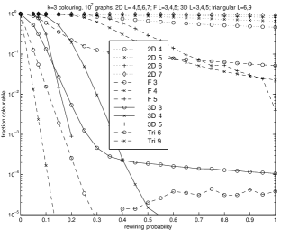
Figure 1: This semilogarithmic plot shows the fraction of colourable graphs as a function of $p$ for various starting lattices. In the legend, “2D”, “F”, “3D”, and “Tri” denote the square, $\gamma=5$ cubic, normal cubic, and triangular starting lattices. The numbers in the legend are the linear size of the lattice. Data were obtained by averaging over from 1000 (for some of the “F” data) to $10^{7}$ different graphs. The differences between the data for graphs with $\gamma=4$, 5, and 6 is clearly seen. See also figures 2 and 3 for detailed comparisons of the different $\gamma$’s.

Figure 1 shows the results for the fraction of colourable graphs for all different start lattices. Notice that this and the other plots are in a semilogarithmic scale. Plot legends describe the lattice and its linear size. The symbol “F” denotes the $\gamma=5$ cubic lattice; thus “F 4” denotes a system of size $N=4^{3}=64$ variables.

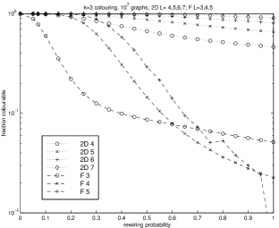
Figure 2: This shows the difference between the square lattice (top curves) and $\gamma=5$ cubic (bottom curves) data. (Same data as in figure 1)

In figure 2 we compare the data for the square and $\gamma=5$ cubic lattices, while figure 3 shows the $\gamma=5$ and $\gamma=6$ data from the runs on the triangular and cubic lattices. The phase transition in solvability can be seen quite clearly in these figures. But note that even for rather large $p$ and $N$, there is still a rather high probability that a $\gamma=5$ graph can be coloured. In fact, the appearance of the $L=3$, 4, and 5 curves seems to indicate that there could be a cross-over at a finite $p$. Unfortunately, the exponential time requirements of the Brelaz algorithm currently prevents us from investigating this in more detail numerically.

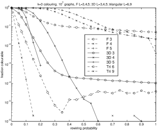
Figure 3: This shows the difference between the $\gamma=5$ cubic (top curves) and $\gamma=6$ cubic and triangular lattice (bottom curves) data. (Same data as in figure 1)

As seen in figure 4, good data collapse can be obtained for the square lattices by plotting the solvable fraction as a function of $pN^{-\nu}$ with $\nu=1.35$. No such collapse can however be obtained for the cubic or triangular data.

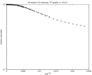
Figure 4: For the data from square ($\gamma=4$) lattices, a good collapse can be obtained by plotting the fraction of colourable graphs as a function of $p^{-\nu}$ with $\nu=3.5$.

In figures 5 and 6, we show the cost (measured as the number of nodes visited in the search-tree) for the runs performed. The $\gamma=5$ graphs prove to be much harder than the others. This is natural since they are closer to the phase transition for random graphs. For the other data, the cost is essentially determined by the number of variables in the problem, independent of which lattice was used as a starting point. The “easy-hard-easy” pattern which can be seen for some of the data in these figures as a function of $p$ is similar to that of k-col on random graphs.

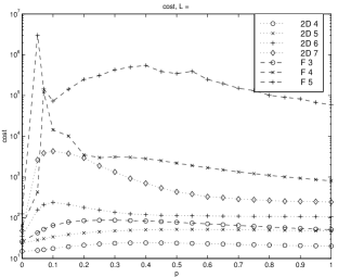
Figure 5: The average cost of determining whether a graph can be coloured or not is also interesting. Here we compare the cost for $\gamma=4$ and $\gamma=5$ as functions of $p$. Note that the cost depends more on the number of variables in the problem than on the coordination number of the graphs. Large system sizes are necessary to see the “easy-hard-easy” transition.

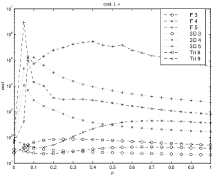
Figure 6: As in figure 5, here we compare the costs for $\gamma=5$ and $\gamma=6$ as functions of $p$. The odd behaviour of the data for triangular lattices is due to finite size effects.

In conclusion, we studied graph colouring on small world graphs produced by starting with regular lattices of coordination number 4, 5, and 6. The hardness patterns found are similar to those for the original small world model. More interestingly, we found that for finite system sizes, there is a range of $p$’s for which the graphs are still colourable even for $\gamma=5$ and 6. We found a new class of problems that are hard for the Brelaz algorithm and could be used as a benchmark for new algorithms. Investigating constraint satisfaction problems on small world graphs and other random graph ensembles with topologies different from that of the standard model ${\cal{G}}(N,\frac{1}{2}\gamma N)$ is important because these graphs might better capture the appearance of real world instances of the problems. For the same reason, it would be interesting to look at other constraint satisfaction problems (such as the vertex-cover problem) on such graphs.

References

- (1) C. H. Papadimitriou, Computational Complexity (Addison-Wesley, Reading, MA, 1994).
- (2) P. Cheeseman, B. Kanefsky, and W. M. Taylor, in Proceedings of IJCAI-91 (Morgan Kauffman, San Mateo, CA, 1991), pp. 331–337.
- (3) T. Hogg, B. A. Huberman, and C. P. Williams, Artificial Intelligence 81, 1 (1996).
- (4) S. Kirkpatrick and B. Selman, Science 264 p 1279 (1994).
- (5) E.g., R. Monasson and R. Zecchina, Phys. Rev. Lett. 76, 3881 (1996); R. Monasson and R. Zecchina, Phys. Rev. E 56, 1357 (1997); R. Monasson, R. Zecchina, S. Kirkpatrick, B. Selman, and L. Troyansky, Nature 400(8) 133 (1999).
- (6) E.g., S. Mertens, Phys. Rev. Lett. 81, 4281 (1998).
- (7) D. Achlioptas and E. Friedgut, Random Structures & Algorithms 14 63-70 (1999).
- (8) D. Achlioptas, “Threshold Phenomena in Random Graph Colouring and Satisfiability”, Ph.D. Thesis, 1999. Available at http://www.research.microsoft.com/optas/.
- (9) B. Bollobás, Random Graphs (Academic Press, New York, 1985).
- (10) D. J. Watts and Steven H. Strogatz, Nature 393 p 440 (1998).
- (11) D. J. Watts, Small Worlds, Princeton University Press 1999.
- (12) M. E. J. Newman, “Models of the Small World: A Review”, e-print cond-mat/0001118.
- (13) M. E. J. Newman, S. H. Strogatz, and D. J. Watts, “Random graphs with arbitrary degree distribution and their applications”, e-print cond-mat/0007235.
- (14) T. Walsh, “’Search in a Small World’, APES Report no 07-1998.
- (15) T. Hogg, in Annual Reviews of Computational Physics (World Scientific, Singapore, 1995), Vol. 2, pp. 357–406.
- (16) D. Brelaz, Comm. ACM 22, 251 (1979).
- (17) D. E. Knuth, Seminumerical Algorithms, Vol. 2 of The Art of Computer Programming, 3 ed. (Addison-Wesley, Reading, MA, 1997).