Integrating Prosodic and Lexical Cues for Automatic Topic Segmentation

Abstract

We present a probabilistic model that uses both prosodic and lexical cues for the automatic segmentation of speech into topically coherent units. We propose two methods for combining lexical and prosodic information using hidden Markov models and decision trees. Lexical information is obtained from a speech recognizer, and prosodic features are extracted automatically from speech waveforms. We evaluate our approach on the Broadcast News corpus, using the DARPA-TDT evaluation metrics. Results show that the prosodic model alone is competitive with word-based segmentation methods. Furthermore, we achieve a significant reduction in error by combining the prosodic and word-based knowledge sources.

1 Introduction

Topic segmentation is the task of automatically dividing a stream of text or speech into topically homogeneous blocks. That is, given a sequence of (written or spoken) words, the aim of topic segmentation is to find the boundaries where topics change. Figure 1 gives an example of a topic change boundary from a broadcast news transcript. Topic segmentation is an important task for various language understanding applications, such as information extraction and retrieval, and text summarization. In this paper, we present our work on automatic detection of topic boundaries from speech input using both prosodic and lexical information.

Other automatic topic segmentation systems have focused on written text and have depended largely on lexical information. This approach is problematic when segmenting speech. Firstly, relying on word identities can propagate automatic speech recognizer errors to the topic segmenter. Secondly, speech lacks typographic cues, as shown in Figure 1: there are no headers, paragraphs, sentence punctuation marks, or capitalized letters. Speech itself, on the other hand, provides an additional, nonlexical knowledge source through its durational, intonational, and energy characteristics, i.e., its prosody.

Prosodic cues are known to be relevant to discourse structure in spontaneous speech (cf. Section 2.3) and can therefore be expected to play a role in indicating topic transitions. Furthermore, prosodic cues by their nature are relatively unaffected by word identity, and should therefore improve the robustness of lexical topic segmentation methods based on automatic speech recognition.

…tens of thousands of people are homeless in northern china tonight after a powerful earthquake hit an earthquake registering six point two on the richter scale at least forty seven people are dead few pictures available from the region but we do know temperatures there will be very cold tonight minus seven degrees $<$TOPIC_CHANGE$>$ peace talks expected to resume on monday in belfast northern ireland former u. s. senator george mitchell is representing u. s. interests in the talks but it is another american center senator rather who was the focus of attention in northern ireland today here’s a. b. c.’s richard gizbert the senator from america’s best known irish catholic family is in northern ireland today to talk about peace and reconciliation a peace process does not mean asking unionists or nationalists to change or discard their identity or aspirations …

Figure 1: An example of a topic boundary in a broadcast news word transcript.

Topic segmentation research based on prosodic information has generally relied on hand-coded cues (with the notable exception of [Hirschberg and Nakatani 1998]), or has not combined prosodic information with lexical cues ([Litman and Passonneau 1995] is one example where lexical information was combined with hand-coded prosodic features for a related task). Therefore, the present work is the first that combines automatic extraction of both lexical and prosodic information for topic segmentation.

The general framework for combining lexical and prosodic cues for tagging speech with various kinds of “hidden” structural information is a further development of our earlier work on sentence segmentation and disfluency detection for spontaneous speech ([Shriberg, Bates, and Stolcke 1997, Stolcke and Shriberg 1996, Stolcke et al. 1998], conversational dialog tagging ([Stolcke et al. 2000], and information extraction from broadcast news ([Hakkani-Tür et al. 1999].

In the next section, we review previous work on topic segmentation. In Section 3, we describe our prosodic and language models as well as methods for combining them. Section 4 reports our experimental procedures and results. We close with some general discussion (Section 5) and conclusions (Section 6).

2 Previous Work

Work on topic segmentation is generally based on two broad classes of cues. On the one hand, one can exploit the fact that topics are correlated with topical content-word usage, and that global shifts in word usage are indicative of changes in topic. Quite independently, discourse cues, or linguistic devices such as discourse markers, cue phrases, syntactic constructions, and prosodic signals are employed by speakers (or writers) as generic indicators of endings or beginnings of topical segments. Interestingly, most previous work has explored either one or the other type of cue, but only rarely both. In automatic segmentation systems, word usage cues are often captured by statistical language modeling and information retrieval techniques. Discourse cues, on the other hand, are typically modeled with rule-based approaches or classifiers derived by machine-learning techniques (such as decision trees).

2.1 Approaches Based on Word Usage

Most automatic topic segmentation work based on text sources has explored topical word usage cues in one form or other. [Kozima 1993] used mutual similarity of words in a sequence of text as an indicator of text structure. [Reynar 1994] presented a method that finds topically similar regions in the text by graphically modeling the distribution of word repetitions. The method of Hearst ([Hearst 1994, Hearst 1997] uses cosine similarity in a word vector space as an indicator of topic similarity.

More recently, the U.S. Defense Advanced Research Projects Agency (DARPA) initiated the Topic Detection and Tracking (TDT) program to further the state of the art in finding and following new topics in a stream of broadcast news stories. One of the tasks in the TDT effort is segmenting a news stream into individual stories. Several of the participating systems rely essentially on word usage: [Yamron et al. 1998] model topics with unigram language models and their sequential structure with hidden Markov models (HMMs). [Ponte and Croft 1997] extract related word sets for topic segments with the information retrieval technique of local context analysis, and then compare the expanded word sets.

2.2 Approaches Based on Discourse and Combined Cues

Previous work on both text and speech has found that cue phrases or discourse particles (items such as now or by the way), as well as other lexical cues, can provide valuable indicators of structural units in discourse ([Grosz and Sidner 1986, Passonneau and Litman 1997, among others].

In the TDT framework, the UMass “HMM” approach described in [Allan et al. 1998] uses an HMM that models the initial, middle, and final sentences of a topic segment, capitalizing on discourse cue words that indicate beginnings and ends of segments. Aligning the HMM to the data amounts to segmenting it.

[Beeferman, Berger, and Lafferty 1999] combined a large set of automatically selected lexical discourse cues in a maximum-entropy model. They also incorporated topical word usage into the model by building two statistical language models: one static (topic independent) and one that adapts its word predictions based on past words. They showed that the log likelihood ratio of the two predictors behaves as an indicator of topic boundaries, and can thus be used as an additional feature in the exponential model classifier.

2.3 Approaches Using Prosodic Cues

Prosodic cues form a subset of discourse cues in speech, reflecting systematic duration, pitch, and energy patterns at topic changes and related locations of interest. A large literature in linguistics and related fields has shown that topic boundaries (as well as similar entities such as paragraph boundaries in read speech, or discourse-level boundaries in spontaneous speech) are indicated prosodically in a manner that is similar to sentence or utterance boundaries—only stronger. Major shifts in topic typically show longer pauses, an extra-high F0 onset or “reset”, a higher maximum accent peak, greater range in F0 and intensity ([Brown, Currie, and Kenworthy 1980, Grosz and Hirschberg 1992, Nakajima and Allen 1993, Geluykens and Swerts 1993, Ayers 1994, Hirschberg and Nakatani 1996, Nakajima and Tsukada 1997, Swerts 1997] and shifts in speaking rate ([Brubaker 1972, Koopmans-van Beinum and van Donzel 1996, Hirschberg and Nakatani 1996]. Such cues are known to be salient for human listeners; in fact, subjects can perceive major discourse boundaries even if the speech itself is made unintelligible via spectral filtering ([Swerts, Geluykens, and Terken 1992].

Work in automatic extraction and computational modeling of these characteristics has been more limited, with most of the work in computational prosody modeling dealing with boundaries at the sentence level or below. However, there have been some studies of discourse-level boundaries in a computational framework. They differ in various ways, such as type of data (monolog or dialog, human-human or human-computer), type of features (prosodic and lexical versus prosodic only), which features are considered available (e.g., utterance boundaries or no boundaries), to what extent features are automatically extractable and normalizable, and the machine learning approach. Because of these vast difference the overall results cannot be compared directly to each other or to our work, but we describe three of the approaches briefly here.

An early study by [Litman and Passonneau 1995] used hand-labeled prosodic boundaries and lexical information, but applied machine learning to a training corpus and tested on unseen data. The researchers combined pause, duration, and hand-coded intonational boundary information with lexical information from cue phrases (such as and and so). Additional knowledge sources included complex relations, such as coreference of noun phrases. Work by [Swerts and Ostendorf 1997] used prosodic features that in principle could be extracted automatically, such as pitch range, to classify utterances from human-computer task-oriented dialog into two categories: initial or noninitial in the discourse segment. The approach used CART-style decision trees to model the prosodic features, as well as various lexical features that could also in principle be estimated automatically. In this case, utterances were presegmented, so the task was to classify segments rather than find boundaries in continuous speech; the features also included some (such as type of boundary tone) that may not be easy to extract robustly across speaking styles. Finally, [Hirschberg and Nakatani 1998] proposed a prosody-only front end for tasks such as audio browsing and playback, which could segment continuous audio input into meaningful information units. They used automatically extracted pitch, energy, and “other” features (such as the cross-correlation value used by the pitch tracker in determining the estimate of F0) as inputs to CART-style trees, and aimed to predict major discourse-level boundaries. They found various effects of frame window length and speakers, but concluded overall that prosodic cues could be useful for audio browsing applications.

3 The Approach

Topic segmentation in the paradigm used in this study and others ([Allan et al. 1998] proceeds in two phases. In the first phase, the input is divided into contiguous strings of words assumed to belong to the same topic. We refer to this step as chopping. For example, in textual input, the natural units for chopping are sentences (as can be inferred from punctuation and capitalization), since we can assume that topics do not change in mid-sentence. For continuous speech input, the choice of chopping criteria is less obvious; we compare several possibilities in our experimental evaluation. Here, for simplicity, we will use sentence to refer to units of chopping, regardless of the criterion used.

In the second phase, the sentences are further grouped into contiguous stretches belonging to one topic, i.e., the sentence boundaries are classified into topic boundaries and nontopic boundaries. Topic segmentation is thus reduced to a boundary classification problem. We will use $B$ to denote the string of binary boundary classifications. Furthermore, our two knowledge sources are the (chopped) word sequence $W$ and the stream of prosodic features $F$. Our approach aims to find the segmentation $B$ with highest probability given the information in $W$ and $F$

$$\mathop{\rm argmax}_{B}P(B|W,F)\quad$$ (1)

using statistical modeling techniques.

In the following subsections, we first describe the prosodic model of the dependency between prosody $F$ and topic segmentation $B$; then, the language model relating words $W$ and $B$; and finally, two approaches for combining the models.

3.1 Prosodic Modeling

The job of the prosodic model is to estimate the posterior probability (or, alternatively, likelihood) of a topic change at a given word boundary, based on prosodic features extracted from the data. For the prosodic model to be effective, one must devise suitable, automatically extractable features. Feature values extracted from a corpus can then be used in training probability estimators and to select a parsimonious subset of features for modeling purposes. We discuss each of these steps in turn in the following sections.

3.1.1 Features

We started with a large collection of features capturing two major aspects of speech prosody, similar to our previous work ([Shriberg, Bates, and Stolcke 1997]:

• Duration features: duration of pauses, duration of final vowels and final rhymes, and versions of these features normalized both for phone durations and speaker statistics.

• Pitch features: fundamental frequency (F0) patterns preceding and following the boundary, F0 patterns across the boundary, and pitch range relative to the speaker’s baseline. We processed the raw F0 estimates (obtained with ESPS signal processing software from [Entropic Research Laboratory 1993]), with robustness-enhancing techniques developed by [Sönmez et al. 1998].

We did not use amplitude- or energy-based features since exploratory work showed these to be much less reliable than duration and pitch and largely redundant given the above features. One reason for omitting energy features is that, unlike duration and pitch, energy-related measurements vary with channel characteristics. Since channel properties vary widely in broadcast news, features based on energy measures can correlate with shows, speakers, and so forth, rather than with the structural locations in which we were interested.

We included features that, based on the descriptive literature, should reflect breaks in the temporal and intonational contour. We developed versions of such features that could be defined at each interword boundary, and that could be extracted by completely automatic means (no human labeling). Furthermore, the features were designed to be as independent of word identities as possible, for robustness to imperfect recognizer output. A brief characterization of the informative features for the segmentation task is given with our results in Section 4.6. Since the focus here is on computational modeling we refer the reader to a companion paper ([Shriberg et al. 2000] for a detailed description of the acoustic processing and prosodic feature extraction.

3.1.2 Decision trees

Any of a number of probabilistic classifiers (such as neural networks, exponential models, or naïve Bayes networks) could be used as posterior probability estimators. As in past prosodic modeling work ([Shriberg, Bates, and Stolcke 1997], we chose CART-style decision trees ([Breiman et al. 1984], as implemented by the IND package ([Buntine and Caruana 1992], because of their ability to model feature interactions, to deal with missing features, and to handle large amounts of training data. The foremost reason for our preference for decision trees, however, is that the learned models can be inspected and diagnosed by human investigators. This ability is crucial for understanding what and how features are used, and for debugging the feature extraction process itself.

Let $F_{i}$ be the features extracted from a window around the $i$th potential topic boundary (chopping boundary), and let $B_{i}$ be the boundary type (boundary/no-boundary) at that position. We trained decision trees to predict the $i$th boundary type, i.e., to estimate $P(B_{i}|F_{i},W)$. The decision is only weakly conditioned on the word sequence $W$, insofar as some of the prosodic features depend on the phonetic alignment of the word models (which we will denote with $W_{\mbox{\scriptsize t}}$). We can thus expect the prosodic model estimates to be robust to recognition errors. The decision tree paradigm also allows us to add, and automatically select, other (nonprosodic) features that might be relevant to the task.

3.1.3 Feature selection

The greedy nature of the decision tree learning algorithm implies that larger initial feature sets can give worse results than smaller subsets. Furthermore, it is desirable to remove redundant features for computational efficiency and to simplify the interpretation of results. For this purpose we developed an iterative feature selection “wrapper” algorithm ([John, Kohavi, and Pfleger 1994] that finds useful, task-specific feature subsets. The algorithm combines elements of a brute-force search with previously determined heuristics about good groupings of features. The algorithm proceeds in two phases: In the first phase, the number of features is reduced by leaving out one feature at a time during tree construction. A feature whose removal increases performance is marked as to be avoided. The second phase then starts with the reduced feature set and performs a beam search over all possible subsets to maximize tree performance.

We used entropy reduction in the overall tree (after cross-validation pruning) as a metric for comparing alternative feature subsets. Entropy reduction is the difference in entropy between the prior class distribution and the posterior distribution estimated by the tree, as measured on a held-out set; it is a more fine-grained metric than classification accuracy, and is also more relevant to the model combination approach described later.

3.1.4 Training data

To train the prosodic model, we automatically aligned and extracted features from 70 hours (about 700,000 words) of the Linguistic Data Consortium (LDC) 1997 Broadcast News (BN) corpus. Topic boundary information determined by human labelers was extracted from the SGML markup that accompanies the word transcripts of this corpus. The word transcripts were aligned automatically with the acoustic waveforms to obtain pause and duration information, using the SRI Broadcast News recognizer ([Sankar et al. 1998].

3.2 Lexical Modeling

Lexical information in our topic segmenter is captured by statistical language models (LMs) embedded in an HMM. The approach is an extension of the topic segmenter developed by Dragon Systems for the TDT2 effort ([Yamron et al. 1998], which was based purely on topical word distributions. We extend it to also capture lexical and (as described in Section 3.3) prosodic discourse cues.

3.2.1 Model structure

The overall structure of the model is that of an HMM ([Rabiner and Juang 1986] in which the states correspond to topic clusters $T_{j}$, and the observations are sentences (or chopped units) $W_{1},\ldots,W_{N}$. The resulting HMM, depicted in Figure 2, forms a complete graph, allowing for transitions between any two topic clusters. Note that it is not necessary that the topic clusters correspond exactly to the actual topics to be located; for segmentation purposes it is sufficient that two adjacent actual topics are unlikely to be mapped to the same induced cluster. The observation likelihoods for the HMM states, $P(W_{i}|T_{j})$, represent the probability of generating a given sentence $W_{i}$ in a particular topic cluster $T_{j}$.

We automatically constructed 100 topic cluster LMs, using the multipass $k$-means algorithm described in [Yamron et al. 1998]. Since the HMM emissions are meant to model the topical usage of words, but not topic-specific syntactic structures, the LMs consist of unigram distributions that exclude stop words (high-frequency function and closed-class words). To account for unobserved words we interpolate the topic cluster-specific LMs with the global unigram LM obtained from the entire training data. The observation likelihoods of the HMM states are then computed from these smoothed unigram LMs.

All HMM transitions within the same topic cluster are given probability one, whereas all transitions between topics are set to a global topic switch penalty (TSP) that is optimized on held-out training data. The TSP parameter allows trading off between false alarms and misses. Once the HMM is trained, we use the Viterbi algorithm ([Viterbi 1967, Rabiner and Juang 1986] to search for the best state sequence and corresponding segmentation. Note that the transition probabilities in the model are not normalized to sum to one; this is convenient and permissible since the output of the Viterbi algorithm depends only on the relative weight of the transition weights.

Figure 2: Structure of the basic HMM developed by Dragon for the TDT Pilot Project. The labels on the arrows indicate the transition probabilities. TSP represents the topic switch penalty.

We augmented the Dragon segmenter with additional states and transitions to also capture lexical discourse cues. In particular, we wanted to model the initial and final sentences in each topic segment, as these often contain formulaic phrases and keywords used by broadcast speakers (From Washington, this is …, And now …). We added two additional states BEGIN and END to the HMM (Figure 3) to model these sentences. Likelihoods for the BEGIN and END states are obtained as the unigram language model probabilities of the initial and final sentences, respectively, of the topic segments in the training data. Note that a single BEGIN and END state are shared for all topics. Best results were obtained by making traversal of these states optional in the HMM topology, presumably because some initial and final sentences are better modeled by the topic-specific LMs.

Figure 3: Structure of an HMM with topic BEGIN and END states. TSP represents the topic switch penalty.

The resulting model thus effectively combines the Dragon and UMass HMM topic segmentation approaches described in [Allan et al. 1998]. In preliminary experiments, we observed a 5% relative reduction in segmentation error with initial and final states over the baseline HMM topology of Figure 2. Therefore, all results reported later use an HMM topology with initial and final states. Note that, since the topic-initial and topic-final states are optional, our training of the model is suboptimal. Instead of labeling all topic-initial and topic-final training sentences as data for the corresponding state, we would expect further improvements by training the HMM in unsupervised fashion using the Baum-Welch algorithm ([Baum et al. 1970, Rabiner and Juang 1986].

3.2.2 Training data

Topic unigram language models were trained from the pooled TDT Pilot and TDT2 training data ([Cieri et al. 1999], covering transcriptions of broadcast news from January 1992 through June 1994 and from January 1998 through February 1998, respectively. These corpora are similar in style, but do not overlap with the 1997 LDC BN corpus from which we selected our prosodic training data and the evaluaton test set. For training the language models we removed stories with fewer than 300 and more than 3000 words, leaving 19,916 stories with an average length of 538 words (including stop words).

3.3 Model Combination

We are now in a position to describe how lexical and prosodic information can be combined for topic segmentation. As discussed before, the LMs in the HMM capture topical word usage as well as lexical discourse cues at topic transitions, whereas a decision tree models prosodic discourse cues. We expect that these knowledge sources are largely independent, so their combination should yield significantly improved performance.

Figure 4: Structure of the final HMM with fictitious boundary states used for combining language and prosodic models. In the figure, states B1, B2, …, B100 represent the presence of a topic boundary, whereas states N1, N2, …, N100 represent topic-internal sentence boundaries. TSP is the topic switch penalty.

Below we present two approaches for building a combined statistical model that performs topic segmentation using all available knowledge sources. For both approaches it is convenient to associate a “boundary” pseudotoken with each potential topic boundary (i.e., with each sentence boundary). Correspondingly, we introduce, into the HMM, new states that emit these boundary tokens. No other states emit boundary tokens; therefore each sentence boundary must align with one of the boundary states in the HMM. As shown in Figure 4, there are two boundary states for each topic cluster, one representing a topic transition and the other representing a topic-internal transition between sentences. Unless otherwise noted, the observation likelihoods for the boundary states are set to unity.

The addition of boundary states allows us to compute the model’s prediction of topic changes as follows: Let ${\bf B}_{1},\ldots,{\bf B}_{C}$ denote the topic boundary states and, similarly, let ${\bf N}_{1},\ldots,{\bf N}_{C}$ denote the nontopic boundary states, where $C$ is the number of topic clusters. Using the forward-backward algorithm for HMMs ([Rabiner and Juang 1986], we can compute $P(q_{i}={\bf B}_{j}|W)$ and $P(q_{i}={\bf N}_{j}|W)$, the posterior probabilities that one of these states is occupied at boundary $i$. The model’s prediction of a topic boundary is simply the sum over the corresponding state posteriors:

$$P_{\mbox{\scriptsize HMM}}(B_{i}={\bf yes}|W) = \sum_{j=1}^{C}P(q_{i}={\bf B}_{j}|W)$$ (2)

$$P_{\mbox{\scriptsize HMM}}(B_{i}={\bf no}|W) = \sum_{j=1}^{C}P(q_{i}={\bf N}_{j}|W)$$

$$= 1-P_{\mbox{\scriptsize HMM}}(B_{i}={\bf yes}|W)$$

3.3.1 Model combination in the decision tree

Decision trees allow the training of a single classifier that takes both lexical and prosodic features as input, provided we can compactly encode the lexical information for the decision tree. We compute the posterior probability $P_{\mbox{\scriptsize HMM}}(B_{i}={\bf yes}|W)$ as shown above, to summarize the HMM’s belief in a topic boundary based on all available lexical information $W$. The posterior value is then used as an additional input feature to the prosodic decision tree, which is trained in the usual manner. During testing, we declare a topic boundary whenever the tree’s overall posterior estimate $P_{\mbox{\scriptsize DT}}(B_{i}|F_{i},W)$ exceeds some threshold. The threshold may be varied to trade off false alarms for miss errors, or to optimize an overall cost function.

Using HMM posteriors as decision tree features is similar in spirit to the knowledge source combination approaches used by [Beeferman, Berger, and Lafferty 1999] and [Reynar 1999], who also used the output of a topical word usage model as input to an overall classifier. In previous work ([Stolcke et al. 1998] we used the present approach as one of the knowledge source combination strategies for sentence and disfluency detection in spontaneous speech.

3.3.2 Model combination in the HMM

An alternative approach to knowledge source combination uses the HMM as the top-level model. In this approach, the prosodic decision tree is used to estimate likelihoods for the boundary states of the HMM, thus integrating the prosodic evidence into the HMM’s segmentation decisions.

More formally, let $Q=(r_{1},q_{1},\ldots,r_{i},q_{i},\ldots,r_{N},q_{N})$ be a state sequence through the HMM. The model is constructed such that the states $r_{i}$ representing topic (or BEGIN/END) clusters alternate with the states $q_{i}$ representing boundary decisions. As in the baseline model, the likelihoods of the topic cluster states ${\bf T}_{j}$ account for the lexical observations:

$$P(W_{i}|r_{i}={\bf T}_{j})=P(W_{i}|T_{j})$$ (4)

as estimated by the unigram LMs. Now, in addition, we let the likelihood of the boundary state at position $i$ reflect the prosodic observation $F_{i}$. Recall that, like $W_{i}$, $F_{i}$ refers to complete sentence units; specifically, $F_{i}$ denotes the prosodic features of the $i$th boundary between such units.

$$\left.\begin{array}[]{rcl}P(F_{i}|q_{i}={\bf B}_{j},W)&=&P(F_{i}|{B_{i}={\bf yes}},W)\\ P(F_{i}|q_{i}={\bf N}_{j},W)&=&P(F_{i}|{B_{i}={\bf no}},W)\end{array}\right\}\mbox{for all $j=1,\ldots,C$}$$ (5)

Using this construction, the product of all state likelihoods will give the overall likelihood, accounting for both lexical and prosodic observations:

$$\prod_{i=1}^{N}P(W_{i}|r_{i})\prod_{i=1}^{N}P(F_{i}|q_{i},W)=P(W,F|Q)$$ (6)

Applying the Viterbi algorithm to the HMM will thus return the most likely segmentation conditioned on both words and prosody, which is our goal.

Although decomposing the likelihoods as shown allows prosodic observations to be conditioned on the words $W$, we use only the phonetic alignment information $W_{t}$ from the word sequence $W$ in our prosodic models, ignoring the word identities, so as to make them more robust to recognition errors.

The likelihoods $P(F_{i}|B_{i},W_{\mbox{\scriptsize t}})$ for the boundary states can now be obtained from the prosodic decision tree. Note that the decision tree estimates posteriors $P_{\mbox{\scriptsize DT}}(B_{i}|F_{i},W_{\mbox{\scriptsize t}})$. These can be converted to likelihoods using Bayes rule as in

$$P(F_{i}|B_{i},W_{\mbox{\scriptsize t}})={P(F_{i}|W_{\mbox{\scriptsize t}})P_{\mbox{\scriptsize DT}}(B_{i}|F_{i},W_{\mbox{\scriptsize t}})\over P(B_{i}|W_{\mbox{\scriptsize t}})}\quad.$$ (7)

The term $P(F_{i}|W_{\mbox{\scriptsize t}})$ is a constant for all decisions $B_{i}$ and can thus be ignored when applying the Viterbi algorithm. Next, we approximate $P(B_{i}|W_{\mbox{\scriptsize t}})\approx P(B_{i})$, justified by the fact that the $W_{\mbox{\scriptsize t}}$ contains only information about start and end times of phones and words, but not directly about word identities. Instead of explicitly dividing the posteriors we prefer to downsample the training set to make $P(B_{i}={\bf yes})=P(B_{i}={\bf no})={1\over 2}$. A beneficial side effect of this approach is that the decision tree models the lower-frequency events (topic boundaries) in greater detail than if presented with the raw, highly skewed class distribution.

As is often the case when combining probabilistic models of different types, it is advantageous to weight the contributions of the language models and the prosodic trees relative to each other. We do so by introducing a tunable model combination weight (MCW), and by using $P_{\mbox{\scriptsize DT}}(F_{i}|B_{i},W_{\mbox{\scriptsize t}})^{\rm MCW}$ as the effective prosodic likelihoods. The value of MCW is optimized on held-out data.

4 Experiments and Results

To evaluate our topic segmentation models we carried out experiments in the TDT paradigm. We first describe our test data and the evaluation metrics used to compare model performance. We then give results obtained with individual knowledge sources, followed by results using the combined models.

4.1 Test Data

We evaluated our system on three hours (6 shows, about 53,000 words) of the 1997 LDC BN corpus. The threshold for the model combination in the decision tree and the topic switch penalty were optimized on the larger development training set of 104 shows, which includes the prosodic model training data. The MCW for the model combination in the HMM was optimized using a smaller held-out set of 10 shows of about 85,000 words total size, separate from the prosodic model training data.

We used two test conditions: forced alignments using the true words, and recognized words as obtained by a simplified version of the SRI Broadcast News recognizer ([Sankar et al. 1998], with a word error rate of 30.5%.

Our aim in these experiments was to use fully automatic recognition and processing wherever possible. For practical reasons, we departed from this strategy in two areas. First, for word recognition, we used the acoustic waveform segmentations provided with the corpus (which also included the location of nonnews material, such as commercials and music). Since current BN recognition systems perform this segmentation automatically with very good accuracy and with only a few percentage points penalty in word error rate ([Sankar et al. 1998], we felt the added complication in experimental setup and evaluation was not justified.

Second, for prosodic modeling, we used information from the corpus markup concerning speaker changes and the identity of frequent speakers (e.g., news anchors). Automatic speaker segmentation and labeling is possible, though with errors ([Przybocki and Martin 1999]. Nevertheless, our use of speaker labels was motivated by the fact that meaningful prosodic features may require careful normalization by speaker, and unreliable speaker information would have made the analysis of prosodic feature usage much less meaningful.

4.2 Evaluation Metrics

We have adopted the evaluation paradigm used by the TDT2—Topic Detection and Tracking Phase 2 ([Doddington 1998] program, allowing fair comparisons of various approaches both within this study and with respect to other recent work. Segmentation accuracy was measured using TDT evaluation software from NIST, which implements a variant of an evaluation metric suggested by [Beeferman, Berger, and Lafferty 1999].

The TDT segmentation metric is different from those used in most previous topic segmentation work, and therefore merits some discussion. It is designed to work on data streams without any potential topic boundaries, such as paragraph or sentence boundaries, being given a priori. It also gives proper partial credit to segmentation decisions that are close to actual boundaries; for example, placing a boundary one word from an actual boundary is considered a lesser error than if the hypothesized boundary is off by, say, 100 words.

The evaluation metric reflects the probability that two positions in the corpus probed at random and separated by a distance of $k$ words are correctly classified as belonging to the same story or not. If the two words belong to the same topic segment, but are erroneously claimed to be in different topic segments by the segmenter, then this will increase the system’s false alarm probability. Conversely, if the two words are in different topic segments, but are erroneously marked to be in the same segment, this will contribute to the miss probability. The false alarm and miss rates are defined as averages over all possible probe positions with distance $k$.

Formally, miss and false alarm rates are computed as

$$P_{\it Miss} = \frac{\sum_{s}\sum_{i=1}^{N_{s}-k}d^{s}_{\it hyp}(i,i+k)\times(1-d^{s}_{\it ref}(i,i+k))}{\sum_{s}\sum_{i=1}^{N_{s}-k}(1-d^{s}_{\it ref}(i,i+k))}$$ (8)

$$P_{\it FalseAlarm} = \frac{\sum_{s}\sum_{i=1}^{N_{s}-k}(1-d^{s}_{\it hyp}(i,i+k))\times d^{s}_{\it ref}(i,i+k)}{\sum_{s}\sum_{i=1}^{N_{s}-k}d^{s}_{\it ref}(i,i+k)}$$ (9)

where the summation is over all broadcast shows $s$ and word positions $i$ in the test corpus and where

$$d^{s}_{\it sys}(i,j)=\left\{\begin{array}[]{ll}1&\mbox{\parbox[t]{216.81pt}{ if words $i$ and $j$ in show $s$ are deemed by {\it sys} to be within the same story}}\\ 0&\mbox{otherwise}\end{array}\right.$$

Here sys can be ref to denote the reference (correct) segmentation, or hyp to denote the segmenter’s decision.

For audio sources an analogous metric is defined where segmentation decisions (same or different topic) are probed at a time-based distance $\Delta$:

$$P_{\it Miss} = \frac{\sum_{s}\int_{t=0}^{T_{s}-\Delta}d^{s}_{\it hyp}(t,t+\Delta)\times(1-d^{s}_{\it ref}(t,t+\Delta)){\rm d}t}{\sum_{s}\int_{t=0}^{T_{s}-\Delta}(1-d^{s}_{\it ref}(t,t+\Delta)){\rm d}t}$$ (10)

$$P_{\it FalseAlarm} = \frac{\sum_{s}\int_{t=0}^{T_{s}-\Delta}(1-d^{s}_{\it hyp}(t,t+\Delta))\times d^{s}_{\it ref}(t,t+\Delta){\rm d}t}{\sum_{s}\int_{t=0}^{T_{s}-\Delta}d^{s}_{\it ref}(t,t+\Delta){\rm d}t}$$ (11)

where the integration is over the entire duration of all stories of the shows in the test corpus, and where

$$d^{s}_{\it sys}(t_{1},t_{2})=\left\{\begin{array}[]{ll}1&\mbox{\parbox[t]{216.81pt}{if times $t_{1}$ and $t_{2}$ in show $s$ are deemed by {\it sys} to be within the same story}}\\ 0&\mbox{otherwise}\end{array}\right.$$

We used the same parameters as used in the official TDT2 evaluation: $k=50$ and $\Delta=15\mbox{ seconds}$. Furthermore, again following NIST’s evaluation procedure, we combine miss and false alarm rates into a single segmentation cost metric

$$C_{\it Seg}=C_{\it Miss}\times P_{\it Miss}\times P_{\it seg}+C_{\it FalseAlarm}\times P_{\it FalseAlarm}\times(1-P_{\it seg})$$ (12)

where the $C_{\it Miss}=1$ is the cost of a miss, $C_{\it FalseAlarm}=1$ is the cost of a false alarm, and $P_{\it Seg}=0.3$ is the a priori probability of a segment being within an interval of $k$ words or $\Delta$ seconds on the TDT2 training corpus.

4.3 Chopping

Unlike written text, the output of the automatic speech recognizer contains no sentence boundaries. Therefore, chopping text into (pseudo)sentences is a nontrivial problem when processing speech. Some presegmentation into roughly sentence-length units is necessary since otherwise the observations associated with HMM states would comprise too few words to give robust likelihoods of topic choice, causing poor performance.

We investigated chopping criteria based on a fixed number of words (FIXED), at speaker changes (TURN), at pauses (PAUSE), and, for reference, at actual sentence boundaries (SENTENCE) obtained from the transcripts. Table 1 gives the error rates for the four conditions, using the true word transcripts of the larger development data set. For the PAUSE condition, we empirically determined an optimal minimum pause duration threshold to use. Specifically, we considered pauses exceeding 0.575 of a second as potential topic boundaries in this (and all later) experiments. For the FIXED condition, a block length of 10 words was found to work best.

 

Table 1: Segmentation error rates for various chopping criteria, using true words of the larger development data set.

  Chopping Criterion $P_{\it Miss}$ $P_{\it FalseAlarm}$ $C_{\it Seg}$ FIXED 0.5688 0.0639 0.2153 TURN 0.6737 0.0436 0.2326 SENTENCE 0.5469 0.0557 0.2030 PAUSE 0.5111 0.0688 0.2002

We conclude that a simple prosodic feature, pause duration, is an excellent criterion for the chopping step, giving comparable or better performance than standard sentence boundaries. Therefore, we used pause duration as the chopping criterion in all further experiments.

4.4 Source-specific Model Tuning

As mentioned earlier, the segmentation models contain global parameters (the topic transition penalty of the HMM and the posterior threshold for the combined decision tree) to trade false alarms for miss errors. Optimal settings for these parameters depend on characteristics of the source, in particular on the relative frequency of topic changes. Since broadcast news programs come from identified sources it is useful and legitimate to optimize these parameters for each show type. We therefore optimized the global parameter for each model to minimize the segmentation cost on the training corpus (after training all other model parameters in a source-independent fashion).

Compared to a baseline using source-independent global TSP and threshold, the source-dependent models showed between 5 and 10% relative error reduction. All results reported below use the source-dependent approach.

4.5 Segmentation Results

Table 2 shows the results for both individual knowledge sources (words and prosody), as well as for the combined models (decision tree and HMM). It is worth noting that the prosody-only results were obtained by running the combined HMM without language model likelihoods; this approach gave better performance than using the prosodic decision trees directly as classifiers.

Both word- and time-based metrics are given; they exhibit generally very similar results. Another dimension of the evaluation is the use of correct word transcripts (forced alignments) versus automatically recognized words. Again, results along this dimension are very similar, with some exceptions noted below.

 

Table 2: Summary of error rates with the language model only (LM), the prosody model only (PM), the combined decision tree (CM-DT), and the combined HMM (CM-HMM). (a) shows word-based error metrics, (b) shows time-based error metrics. In both cases a “chance” classifier that labels all potential boundaries as nontopic would achieve 0.3 weighted segmentation cost.

 

• 	Error Rates on Forced Alignments			Error Rates on Forced Alignments
  Model	$P_{\it Miss}$	$P_{\it FalseAlarm}$	$C_{\it Seg}$	$P_{\it Miss}$	$P_{\it FalseAlarm}$	$C_{\it Seg}$
  Chance	1.0	0.0	0.3	1.0	0.0	0.3
  LM	0.4847	0.0630	0.1895	0.4978	0.0577	0.1897
  PM	0.4130	0.0596	0.1657	0.4125	0.0705	0.1731
  CM-DT	0.4677	0.0260	0.1585	0.4891	0.0146	0.1569
  CM-HMM	0.3339	0.0536	0.1377	0.3748	0.0450	0.1438

• 	Error Rates on Forced Alignments			Error Rates on Forced Alignments
  Model	$P_{\it Miss}$	$P_{\it FalseAlarm}$	$C_{\it Seg}$	$P_{\it Miss}$	$P_{\it FalseAlarm}$	$C_{\it Seg}$
  Chance	1.0	0.0	0.3	1.0	0.0	0.3
  LM	0.5260	0.0490	0.1921	0.5361	0.0415	0.1899
  PM	0.3503	0.0892	0.1675	0.3846	0.0737	0.1669
  CM-DT	0.5136	0.0210	0.1688	0.5426	0.0125	0.1715
  CM-HMM	0.3426	0.0496	0.1375	0.3746	0.0475	0.1456

Comparing the individual knowledge sources, we observe that prosody alone does somewhat better than the word-based HMM alone. The types of errors made differ consistently: the prosodic model has a higher false alarm rate, while the word-LMs have more miss errors. The prosodic model shows more false alarms because many regular sentence boundaries often show characteristics similar to those of topic boundaries. It also suggests that both models could be combined by letting the prosodic model selects candidate topic boundaries that are then filtered using lexical information.

The combined models generally improve on the individual knowledge sources. In the word-based evaluation, the combined decision tree (DT) reduced overall segmentation cost by 19% over the language model on true words (17% on recognized words). The combined HMM gave even better results: 27% and 24% improvement in the error rate over the language model for the true and recognized words, respectively.

Looking again at the breakdown of errors, we can see that the two model combination approaches work quite differently: the combined DT has about the same miss rate as the LM, but lower false alarms. The combined HMM, by contrast, combines a miss rate as low as (or lower than) that of the prosodic model with the lower false alarm rate of the LM, suggesting that the functions of the two knowledge sources are complementary, as discussed above. Furthermore, the different error patterns of the two combination approaches suggest that further error reductions could be achieved by combining the two hybrid models.

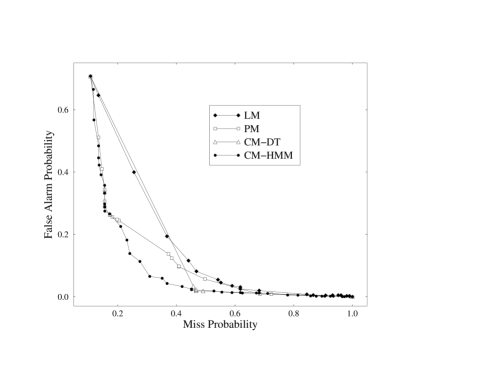
Figure 5: False alarm versus miss probabilities (word-based metrics) for automatic topic segmentation from known words (forced alignments). The segmenters used were a words-only HMM (LM), a prosody-only HMM (PM), a combined decision tree (CM-DT), and a combined HMM (CM-HMM).

The trade-off between false alarms and miss probabilities is shown in more detail in Figure 5, which plots the two error metrics against each other. Note that the false alarm rate does not reach 1 because the segmenter is constrained by the chopping algorithm: the pause criterion prevents the segmenter from hypothesizing topic boundaries everywhere.

4.6 Decision Tree for the Prosody-only Model

Figure 6: The decision tree using prosodic features only.

Feature subset selection was run with an initial set of 73 potential features, which the algorithm reduced to a set of 7 nonredundant features helpful for the topic segmentation task. The full decision tree learned is shown in Figure 6. We can identify four different kinds of features used in the tree, listed below. For each feature type, we give the feature names found in the tree and the relative feature usage, an approximate measure of feature importance ([Shriberg, Bates, and Stolcke 1997]. Relative feature usage is computed as the relative frequency with which features of a given type are queried in the tree, over a held-out test set.

1. Pause duration (PAU_DUR, 42.7% usage). This feature is the duration of the nonspeech interval occurring at the boundary. The importance of pause duration is underestimated here because, as explained earlier, pause durations are already used during the chopping process, so that the decision tree is applied only to boundaries exceeding a certain duration. Separate experiments using boundaries below our chopping threshold show that the tree also distinguishes shorter pause durations for segmentation decisions.

2. F0 differences across the boundary (F0K_LR_MEAN_KBASELN and F0K_WRD_DIFF_MNMN_NG, 35.9% usage). These features compare the mean F0 of the word preceding the boundary (measured from voiced regions within that word) to either the speaker’s estimated baseline F0 (F0K_LR_MEAN_KBASELN) or to the mean F0 of the word following the boundary (F0K_WRD_DIFF_MNMN_N). Both features were computed based on a log-normal scaling of F0. Other measures (such as minimum or maximum F0 in the word or preceding window) as well as other normalizations (based on F0 toplines, or non-log-based scalings) were included in the initial feature set, but were not selected in the best-performing tree. The baseline feature captures a pitch range effect, and is useful at boundaries where the speaker changes (since range here is compared only within-speaker). The second feature captures the relative size of the pitch change at the boundary, but of course is not meaningful at speaker boundaries.

3. Turn features (TURN_F and TURN_TIME, 14.6% usage). These features reflect the change of speakers. TURN_F indicates whether a speaker change occurred at the boundary, while TURN_TIME measures the time passed since the start of the current turn.

4. Gender (GEN, 6.8% usage). This feature indicates the speaker gender right before a potential boundary.

Inspection of the tree reveals that the purely prosodic features (pause duration and F0 differences) are used as the prosody literature suggests. The longer the observed pause, the more likely a boundary corresponds to a topic change. Also, the closer a speaker comes to his or her F0 baseline, or the larger the difference to the F0 following a boundary, the more likely a topic change occurs. These features thus correspond to the well-known phenomena of boundary tones and pitch reset that are generally associated with sentence boundaries ([Vaissière 1983]. We found these indicators of sentences boundaries to be particularly pronounced at topic boundaries.

While turn and gender features are not prosodic features per se, they do interact closely with them since prosodic measurements must be informed by and carefully normalized for speaker identity and gender, and it is therefore natural to include them in a prosodic classifier. Not surprisingly, we find that turn boundaries are positively correlated with topic boundaries, and that topic changes become more likely the longer a turn has been going on.

Interestingly, speaker gender is used by the decision tree for several reasons. One reason is stylistic differences between males and females in the use of F0 at topic boundaries. This is true even after proper normalization, e.g., equating the gender-specific nontopic boundary distributions. In addition, we found that nontopic pauses (i.e., chopping boundaries) are more likely to occur in male speech. It could be that male speakers in BN are assigned longer topic segments on average, or that male speakers are more prone to pausing in general, or that male speakers dominate the spontaneous speech portions, where pausing is naturally more frequent. The details of this gender effect await further study.

4.7 Decision Tree for the Combined Model

Figure 7: The decision tree of the combination model.

Figure 7 depicts the decision tree that combines the HMM language model topic decisions with prosodic features (see Section 3.3.1). Again, we list the features used with their relative feature usages.

1. Language model posterior (POST_TOPIC, 49.3% usage). This is the posterior probability $P(B_{i}={\bf yes}|W)$ computed from the HMM.

2. Pause duration (PAU_DUR, 49.3% usage). This feature is the same as described for the prosody-only model.

3. F0 differences across the boundary (F0K_WRD_DIFF_HILO_N and F0K_LR_MEAN_KBASELN, 1.4% usage). These features are similar to those found for the prosody-only tree. The only difference is that for the first feature, the comparison of F0 values across the boundary is done by taking the maximum F0 of the previous word and the minimum F0 of the following word—rather than the mean for both cases.

The decision tree found for the combined task is smaller and uses fewer features than the one trained with prosodic features only, for two reasons. First, the LM posterior feature is found to be highly informative, superseding the selection of many of the low-frequency features previously found. Furthermore, as explained in Section 3.3.2, the prosody-only tree was trained on a downsampled dataset that equalizes the priors for topic and nontopic boundaries, as required for integration into the HMM. A welcome side effect of this procedure is that it forces the tree to model the less frequent class (topic boundaries) in much greater detail than if the tree were trained on the raw class distribution, as is the case here.

Because of its small size, the tree in Figure 7 is particularly easy to interpret. The top-level split is based on the LM posterior. The right branch handles cases where words are highly indicative of a topic boundary. However, for short pauses the tree queries further prosodic features to prevent false alarms. Specifically, short pauses must be accompanied both by an F0 close to the speaker’s baseline and by a large F0 reset to be deemed topic boundaries. Conversely, if the LM posteriors are low (left top-level branch), but the pause is very long, the tree still outputs a topic boundary.

4.8 Comparison of Model Combination Approaches

Results indicate that the model combination approach using an HMM as the top-level model works better than the combined decision tree. While this result deserves more investigation we can offer some preliminary insights.

We found it difficult to set the posterior probability thresholds for the combined decision tree in a robust way. As shown by the “CM-DT” curve in Figure 5, there is a large jump in the false alarm/miss trade-off for the combined tree, in contrast to the combined HMM approach, which controls the trade-off by a changing topic switch penalty. This occurs because posterior probabilities from the decision tree do not vary smoothly; rather, they vary in steps corresponding to the leaves of the tree. The discontinuous character of the thresholded variable makes it hard to estimate a threshold on the training data that performs robustly on the test data. This could account for the poor result on the time-based metrics for the combined tree (where the threshold optimized on the training data was far from optimal on the test set; see footnote 8). The same phenomenon is reflected in the fact that the prosody-only tree gave better results when embedded in an HMM without LM likelihoods than when used by itself with a posterior threshold.

4.9 Contributions of Different Feature Types

We saw in Section 4.6 that pause duration is by far the single most important feature in the prosodic decision tree. Furthermore, speaker changes are queried almost as often as the F0-related features. Pause durations can be obtained using standard speech recognizers, and are in fact used by many current TDT systems (see Section 4.10). Speaker changes are not prosodic features per se, and would be detected independently from the prosodic features proper. To determine if prosodic measurements beyond pause and speaker information improve topic segmentation accuracy, we tested systems that consisted of the HMM with the usual topic LMs, plus a decision tree that had access only to various subsets of pause- and speaker-related features, without using any of the F0-based features. Decision tree and HMM were combined as described in Section 3.3.2.

 

Table 3: Segmentation error rates with the language model only (LM), the combined HMM using all prosodic features (CM-HMM-all), the combined HMM using only pause duration and turn features (CM-HMM-pause-turn), and using only pause-duration, turn, and gender features (CM-HMM-pause-turn-gender).

  Model $C_{seg}$ LM 0.1895 CM-HMM-pause-turn 0.1519 CM-HMM-pause-turn-gender 0.1511 CM-HMM-all 0.1377

Table 3 shows the results of the system using only topic language models (LM) as well as combined systems using all prosodic features (CM-HMM-all), only pause duration and turn features (CM-HMM-pause-turn), and using only pause duration, turn, and gender features (CM-HMM-pause-turn-gender). These results show that by using only pause duration, turn, and gender features, it is indeed possible to obtain better results (20% reduced segmentation cost) than with the lexical model alone, with gender making only a minor contribution. However, we also see that a substantial further improvement (9% relative) is obtained by adding F0 features into the prosodic model.

4.10 Results Compared to Other Approaches

Because our work focused on the use of prosodic information and required detailed linguistic annotations (such as sentence punctuation, turn boundaries, and speaker labels), we used data from the LDC 1997 BN corpus to form the training set for the prosodic models and the (separate) test set used for evaluation. This choice was crucial for the research, but unfortunately complicates a quantitative comparison of our results to other TDT segmentation systems. The recent TDT2 evaluation used a different set of broadcast news data that postdated the material used by us, and was generated by a different speech recognizer (although with a similar word error rate) ([Cieri et al. 1999]. Nevertheless we have attempted to calibrate our results with respect to these TDT2 results. We have not tried to compare our results to research outside the TDT evaluation framework. In fact, other evaluation methodologies differ too much to allow meaningful quantitative comparisons across publications.

We wanted to ensure that the TDT2 evaluation test set was comparable in segmentation difficulty to our test set drawn from the 1997 BN corpus, and that the TDT2 metrics behaved similarly on both sets. To this end, we ran an early version of our words-only segmenter on both test sets. As shown in Table 4, not only are the results on recognized words quite close, but the optimal false alarm/miss trade-off is similar as well, indicating that the two corpora have roughly similar topic granularities.

 

Table 4: Word-based segmentation error rates for different corpora. Note that a hand-transcribed (forced alignment) version of the TDT2 test set was not available.

  Error Rates on Forced Alignments Error Rates on Forced Alignments Test Set $P_{\it Miss}$ $P_{\it FalseAlarm}$ $C_{\it Seg}$ $P_{\it Miss}$ $P_{\it FalseAlarm}$ $C_{\it Seg}$ TDT2 NA NA NA 0.5509 0.0694 0.2139 BN’97 0.4685 0.0817 0.1978 0.5128 0.0683 0.2017

While the full prosodic component of our topic segmenter was not applied to the TDT2 test corpus, we can compare the performance of a simplified version of SRI’s segmenter to other evaluation systems ([Fiscus et al. 1999]. The two best-performing systems in the evaluation were those of CMU ([Beeferman, Berger, and Lafferty 1999] with $C_{\it Seg}=0.1463$, and Dragon ([Yamron et al. 1998, van Mulbregt et al. 1999] with $C_{\it Seg}=0.1579$. The SRI system achieved $C_{\it Seg}=0.1895$. All systems in the evaluation, including ours, used only information from words and pause durations determined by a speech recognizer.

A good reference to calibrate our performance is the Dragon system, from which we borrowed the lexical HMM segmentation framework. Dragon made adjustments in its lexical modeling that account for the improvements relative to the basic HMM structure on which our system is based. As described by [van Mulbregt et al. 1999], a significant segmentation error reduction was obtained from optimizing the number of topic clusters (kept fixed at 100 in our system). Second, Dragon introduced more supervision into the model training by building separate LMs for segments that had been hand-labeled as not related to news (such as sports and commercials) in the TDT2 training corpus, which also resulted in substantial improvements. Finally, Dragon used some of the TDT2 training data for tuning the model to the specifics of the TDT2 corpus.

In summary, the performance of our combined lexical-prosodic system with $C_{\it Seg}=0.1438$ is competitive with the best word-based systems reported to date. More importantly, since we found the prosodic and lexical knowledge sources to complement each other, and since Dragon’s improvements for TDT2 were confined to a better modeling of the lexical information, we would expect that adding these improvements to our combined segmenter would lead to a significant improvement in the state of the art.

5 Discussion

Results so far indicate that prosodic information provides an excellent source of information for automatic topic segmentation, both by itself and in conjunction with lexical information. Pause duration, a simple prosodic feature that is readily available as a by-product of speech recognition, proved highly effective in the initial chopping phase, as well as being the most important feature used by prosodic decision trees. Additional, pitch-based prosodic features are also effective as features in the decision tree.

The results obtained with recognized words (at 30% word error rate) did not differ greatly from those obtained with correct word transcripts. No significant degradation was found with the words-only segmentation model, while the best combined model exhibited about a 5% error increase with recognized words. The lack of degradation on the words-only model may be partly due to the fact that the recognizer generally outputs fewer words than contained in the correct transcripts, biasing the segmenter toward a lower false alarm rate. Still, part of the appeal of prosodic segmentation is that it is inherently robust to recognition errors. This characteristic makes it even more attractive for use in domains with higher error rates due to poor acoustic conditions or more conversational speaking styles. It is especially encouraging that the prosody-only segmenter achieved competitive performance.

It was fairly straightforward to modify the original Dragon HMM segmenter ([Yamron et al. 1998], which is based purely on topical word usage, to incorporate discourse cues, both lexical and prosodic. The addition of these discourse cues proved highly effective, especially in the case of prosody. The alternative knowledge source combination approach, using HMM posterior probabilities as decision tree inputs, was also effective, although less so than the HMM-based approach. Note that the HMM-based integration, as implemented here, makes more stringent assumptions about the independence of lexical and prosodic cues. The combined decision tree, on the other hand, has some ability to model dependencies between lexical and prosodic cues. The fact that the HMM-based combination approach gave the best results is thus indirect evidence that lexical and prosodic knowledge sources are indeed largely independent.

• …we have a severe thunderstorm watch two severe thunderstorm watches and a tornado watch in effect the tornado watch in effect back here in eastern colorado the two severe thunderstorm watches here indiana over into ohio those obviously associated with this line which is already been producing some hail i’ll be back in a moment we’ll take a look at our forecast weather map see if we can cool it off in the east will be very cold tonight minus seven degrees $<$TOPIC_CHANGE$>$ LM probability: 0.018713
  PM probability: 0.937276
  karen just walked in was in the computer and found out for me that national airport in washington d. c. did hit one hundred degrees today it’s a record high for them it’s going to be uh hot again tomorrow but it will begin to cool off the que question is what time of day is this cold front going to move by your house if you want to know how warm it’s going to be tomorrow comes through early in the day won’t be that hot at all midday it’ll still be into the nineties but not as hot as it was today comes through late in the day you’ll still be in the upper nineties but some relief is on the way …

• …you know the if if the president has been unfaithful to his wife and at this point you know i simply don’t know any of the facts other than the bits and pieces that we hear and they’re simply allegations at this point but being unfaithful to your wife isn’t necessarily a crime lying in an affidavit is a crime inducing someone to lie in an affidavit is a crime but that occurred after this apparent taping so i’ll tell you there are going to be extremely thorny legal issues that will have to be sorted out white house spokesman mike mccurry says the administration will cooperate in starr’s investigation $<$TOPIC_CHANGE$>$ LM probability: 1.000000 PM probability: 0.134409
  cubans have been waiting for this day for a long time after months of planning and preparation pope john paul the second will make his first visit to the island nation this afternoon it is the first pilgrimage ever by a pope to cuba judy fortin joins us now from havana with more …

Figure 8: Examples of true topic boundaries where lexical and prosodic models make opposite decisions. (a) The prosodic model correctly predicts a topic change, the LM does not. (b) The LM predicts a topic change, the prosodic model does not.

Apart from the question of probabilistic independence, it seems that lexical and prosodic models are also complementary in the errors they make. This is manifested in the different distributions of miss and false alarm errors discussed in Section 4.5. It is also easy to find examples where the two models make complementary errors. Figure 8 shows two topic boundaries that are missed by one model but not the other.

Several aspects of our model are preliminary or suboptimal in nature and can be improved. Even when testing on recognized words, we used parameters optimized on forced alignments. This is suboptimal but convenient, since it avoids the need to run word recognition on the relatively large training set. Since results on recognized words are very similar to those on true words we can conclude that not much was lost with this expedient. Also, we have not yet optimized the chopping stage relative to the combined model (only relative to the words-only segmenter). The use of prosodic features other than pause duration for chopping should further improve the overall performance.

The improvement obtained with source-dependent topic switch penalties and posterior thresholds suggests that more comprehensive source-dependent modeling would be beneficial. In particular, both prosodic and lexical discourse cues are likely to be somewhat source specific (e.g., because of different show formats and different speakers). Given enough training data, it is straightforward to train source-dependent models.

6 Conclusion

We have presented a probabilistic approach for topic segmentation of speech, combining both lexical and prosodic cues. Topical word usage and lexical discourse cues are represented by language models embedded in an HMM. Prosodic discourse cues, such as pause durations and pitch resets, are modeled by a decision tree based on automatically extracted acoustic features and alignments. Lexical and prosodic features can be combined either in the HMM or in the decision tree framework.

Our topic segmentation model was evaluated on broadcast news speech, and found to give competitive performance (around 14% error according to the weighted TDT2 segmentation cost metric). Notably, the segmentation accuracy of the prosodic model alone is competitive with a word-based segmenter, and a combined prosodic/lexical HMM achieves a substantial error reduction over the individual knowledge sources.

Acknowledgments

We thank Becky Bates, Madelaine Plauché, Ze’ev Rivlin, Ananth Sankar, and Kemal Sönmez for invaluable assistance in preparing the data for this study. The paper was greatly improved as a result of comments by Andy Kehler, Madelaine Plauché, and the anonymous reviewers. This research was supported by DARPA and NSF under NSF grant IRI-9619921 and DARPA contract no. N66001-97-C-8544. The views herein are those of the authors and should not be interpreted as representing the policies of the funding agencies.

References

- [Allan et al. 1998] Allan, J., J. Carbonell, G. Doddington, J. Yamron, and Y. Yang. 1998. Topic detection and tracking pilot study: Final report. In Proceedings DARPA Broadcast News Transcription and Understanding Workshop, pages 194–218, Lansdowne, VA, February. Morgan Kaufmann.
- [Ayers 1994] Ayers, Gayle M. 1994. Discourse functions of pitch range in spontaneous and read speech. In Working Papers in Linguistics No. 44. Ohio State University, pages 1–49.
- [Baum et al. 1970] Baum, Leonard E., Ted Petrie, George Soules, and Norman Weiss. 1970. A maximization technique occurring in the statistical analysis of probabilistic functions in Markov chains. The Annals of Mathematical Statistics, 41(1):164–171.