-
Lectures on Reduce and Maple
at UAM-I, Mexico 111see also www.thp.uni-koeln.de/~mt/work/1999mexico/
-
list
Computer Algebra (CA)
In order to get an idea what facilities CA provides it might be sensible to ask what we expect from CA. I suggest that
CA is supposed to solve or simplify any algebraic problem that we can state explicitly.
So, CA has to provide methods to simplify algebraic expression and to solve equation systems. This, of course, is not enough because it also has enable us to input our problem and has to generate some output of the result (also graphical, plots, LaTeX, etc.). I want to differentiate the needs for the input a little bit more: On the one hand, CA has to offer some language or formalism that includes many operators to form expressions (, etc.) and on the other it should provide methods to make definitions, declarations, substitutions, and assumptions. Thus, we split the facilities we expect from CA into four groups:
-
A
operators to form expressions
-
B
methods to make definitions, declarations, substitution, and assumptions
-
C
methods to simplify and solve
-
D
methods to generate output
The reason why I suggest this splitting of the commands is the following: It seems that the discussion of group A dominates most handbooks on CA only because it is by far the largest group of commands and operators. I find though, that the commands in group B and C are more elementary and important to understand whereas for the commands in group A one can well refer to the online user’s manual. The commands in group D are also important for efficient work with CA. This is why these lectures try to emphasize the commands in groups B, C, and D a little bit more than usual.
Chapter 1 Reduce I
1.1 The simplification principle
As stated, I think the simplification and solving methods of a CA system to be most elementary and important. Hence we start to discuss these in the case of Reduce.
Reduce is an input-output machine. One could say that all that Reduce does is to reformulate your input expression obeying certain rules! One of these rules is, e.g., to execute all operators and commands in the expression. For example, Reduce reformulates by executing the operator and answering . Fortunately, the rules for reformulation are such that - usually - this reformulation means a simplification. These rules can be influenced by the user: Either by switching on and off the rule switches or by introducing new rules. Most important, Reduce offers the rule switches collected in table 1.1.
switch description e.g. * allfac factorize simple factors div divide by the denominator * exp expand all expressions * mcd make (common) denominators * lcm cancel least common multiples gcd cancel greatest common divisor rat display as polynomial in factor * ratpri display rationals as fraction * pri dominates allfac, div, rat, revpri revpri display polynomials in opposite order rounded calulate with floats complex simplify complex expressions nero don’t display zero results * nat display in Reduce input format **2/3 msg suppress messages fort display in Fortran format tex display in TeX format Table 1.1: Switches for Reduce’s reformulation rules. Those marked with * are turned on at default. As one can see, by switching on the exp-rule, Reduce reformulates and thus simplifies the expression as . This principle is quite different to other CA systems. The combination of such rules can be very powerful. The rule switches turned on at default are: allfac, exp, mcd, lcm, ratpri, pri, nat. This means that, at default, for any expression (subexpression, component, etc. ), Reduce expands the multiplication of two larger terms, interprets all divisions as rationals, tries to divide common factors in numerators and denominators, and finally tries to factorize simple factors. This is already quite a powerful simplification scheme.
1.2 The interface
Starting Reduce on Unix it displays about
Loading image file:
  /vol/sc/lib/reduce3.6_patch980830/reduce.img REDUCE 3.6, 15-Jul-95,
  patched to 30 Aug 98 ...

1:
The first three lines are an artifact of Reduce being implemented in LISP: The program code (image) of Reduce is passed to the LISP interpretor. The prompt 1: expects a command as input. Reduce ignores all upper case letters! A command consists out of a statement and a terminator. The terminator decides whether the Reduce’s response is displayed (; terminator) or not ($ terminator). The following lines are command lines only, the response of Reduce is (sometimes) indicated after the comments sign %. All examples in this chapter are collected in the file red1 at [5].
% file "red1"

off factor, exp, mcd, ratpri$
(x+1)**3/3 - x;                %-> 1/3*(x + 1)**3 - x
on mcd$          ws;           %-> ((x + 1)**3 - 3*x)/3
on ratpri$       ws;           %->
on exp$          ws;           %-> (x**3 + 3*x**2 + 1)/3
factor x$on rat$ ws;           %-> x**3/3 + x**2 + 1/3
remfac x$off exp$

z+a;                           %-> a + z
order z,a$ ws;                 %-> z + a
order nil$ ws;                 %-> a + z
1.3 User definitions
1.3.1 Names and assignments
off mcd$
my_name123 := (x**2-1)/(x+1);  %-> my_name123 := (x + 1)**(-1)*(x**2 - 1)
on mcd$ my_name123;            %-> x - 1
clear my_name123;
A string can be used as a name (or identifier) for variables, procedures, etc. The first character of a name has to be alphabetic, whereas others can be numbers or ’_’, e.g. ’a11’ and ’ric_scalar0’ are proper names. A name should not coincide with a reserved variable name (e i infinity nil pi t) or the command names in table 1.2.
As long as a name is not assigned to some (symbolic) value it is considered to be a clear name. The assignment operator
name:=expr;
assigns the (reformulated) expression on the rhs to the name on the lhs. To withdraw an assignment one uses the command
clear name;
This command also deallocates the memory resource that is associated with the name.
For understanding Reduce, it is important to distinguish between the expression assigned to a name and the value that Reduce displays when evaluating the name. The last of which was reformulated by Reduce with current rules and definitions:
a:=b$ a;                       %-> b
b:=1$ a;                       %-> 1
a:=a$b:=2$ a;                  %-> 1
clear a,b;
In the first line, a is assigned to b and is, of course, also evaluated to be b. In the second line, a is still assigned to b but is evaluated to be 1 (because b is assigned to 1). In the third line, a is assigned to 1 (because the rhs a is evaluated to be 1) and an thus it is also evaluated to be 1 even after b is assigned to 2. We see that the reassignment (a:=a$) is not trivial at all! Analogously, the following example shows the importance of the reassignment if rules have changed:
off mcd$ a:=(x**2-1) / (x-1);     %-> a := (x**2 - 1)*(x - 1)**(-1)
on mcd$  a := a$  a;              %-> x + 1
off mcd$ a;                       %-> x + 1
Here, in the end, a is assigned to x+1. Without the reassignment a:=a$, a would still be assigned to (x**2 - 1)*(x - 1)**(-1) and also evaluated to be such in the last line.
The reassignment is one of the most important tools to apply new definitions and to use the simplification methods of Reduce.
1.3.2 Aliases
To define aliases for any expression, one can use the define command. The syntax is
define alias=expression;
Note that the rhs expression is evaluated before it is assigned to the alias. However: An alias can never ever be changed or unassigned during a Reduce session! If an alias appears in an expression it is replaced by its associated value before Reduce applies any other rules. Example:
define isprime = primep;
for x:=0:20 do if isprime(x) then write x," is a prime!";
                                       % throws 2 3 5 7 11 13 17 19

define is_assigned_to = :=;
x is_assigned_to 5;                    %-> x := 5
1.3.3 Substitutions
Actually, we already noticed how to substitute identities into expressions: Define the identity with an assignment statement or introduce a rule for this identity. Then reevaluate the expression. Say, e.g., we want to substitute into , then we could write one of the following three lines:
f := cos(x)$ x:=0$            f; clear x$        %-> 1
f := cos(x)$ let { x=>0 }$    f; clear x$        %-> 1
f := cos(x)$ f where { x=>0 };                   %-> 1
f := cos(x)$ sub(x=0,f);                         %-> 1
The last possibility is the most beautiful, because one does not have to clear the assignment x:=0 or the rule x=>0 hereafter. The where command only introduces a local rule. After these substitutions, f is still assigned to cos(x) but was only locally evaluated to be 1. Reduce also offers the match command to substitute expressions for polynomials instead of names.
1.3.4 Rules
In the upper example we already introduced the let command that introduces new rules. In general, a rule has syntax
expr => expr [when boolean]
and the let command accepts a list of rules as parameter. Rules can be of explicit nature where any literal occurrence of the lhs expression is replaced by the rhs expression. Or they can by of parametric nature where the lhs expression includes formal names (like parameters) that represent any expressions. These formal names are marked with a twiddle such as ~x:
sin(x)**2 + cos(x)**2;         %-> cos(x)**2 + sin(x)**2
trig_rules:={
 cos(~x)*cos(~y) => (1/2)*(cos(x+y)+cos(x-y)),
 sin(~x)**2 + cos(~x)**2 => 1 }$
let trig_rules$
sin(x+1)**2 + cos(x+1)**2;     %-> 1
cos(pi/3-1) * cos(1);          %-> (2*cos((pi - 6)/3) + 1)/4
showrules cos;                 % shows ALL rules associated with cos!
clearrules trig_rules;
As already mentioned, the where command applies rules only one the preceding expression. The command
showrules name;
displays all rules associated with the name. This gives an insight in how Reduce defines functionals:
1: showrules log;

{log(1) => 0,

 log(e) => 1,

      ~x
 log(e  ) => x,

                    1
 df(log(~x),~x) => ---}
                    x
1.3.5 Operators
An operator is any name that accepts parameters. In Reduce, one can declare a name to be an operator without at all specifying how many parameters the operator expects and what the functionality of the operator is! This leaves the user large freedom to handle and use operators. E.g., one can introduce indexed coordinates by declaring to be an operator with the index as only parameter and without any further properties. In fact, most other, more specialized declarations (like matrix, procedure, etc.) can be thought of special kinds of operator declarations. And also functions (such as sin, log, etc.) can be introduced as operators with certain properties. The properties of an operator are declared by specifying the rules how Reduce has to handle them. Example:
operator eps$                  % declares a new operator
antisymmetric eps$             % declares eps to be totally antisymmetric
let { eps(0,1,2,3) => 1  }$    % defines the properties of this operator
eps(3,1,2,0); eps(2,0,1,1);    %-> -1 and 0
showrules eps;                 %-> {eps(3,2,1,0) => 1}$
clear my_sin$ operator my_sin$ my_sin_rules:={ my_sin(~x) => - my_sin(-x) when numberp(x/pi) and x/pi<0, my_sin(~x) => my_sin(x - 2*pi) when numberp(x/pi) and x/pi>2, my_sin(~x) => - my_sin(x - pi) when numberp(x/pi) and x/pi>1, my_sin(~x) => my_sin(pi - x) when numberp(x/pi) and x/pi>1/2, my_sin(0) => 0, my_sin(pi/6) => 1/2, my_sin(pi/4) => 1/2*sqrt(2), my_sin(pi/3) => 1/2*sqrt(3), my_sin(pi/2) => 1 }$ let my_sin_rules$ my_sin(-124*pi/6); %-> - sqrt(3)/2 clearrules my_sin_rules;1.4 Solving
solve(x**3-3*x**2-61*x+63,x);  %-> {x=9,x=1,x=-7} which are the nulls of this polynomial
solve({x+y-9,-2*y**2+3*x},{x,y});   %-> { {y= - 9/2,x=27/2} , {y=3,x=6} }
Reduce tries to solve algebraic equation systems with
solve(expr_list,name_list);
Without the switch multiplicities Reduce display multiple solutions only once.
Reduce has no build-in routines to solve differnential equations. However, there exist packages for this problem. One should especially mention the CATHODE 2 project (Computer Algebra Tools for Handling Ordinary Differential Equations) which develops routines to hande differential equation systems also for Reduce. The members of this group are M. MacCallum (London), V. Fairen (Madrid), E. Tournier (Grenoble), Th. Mulders (Zurich), M. van der Puf (Groningen), F. Schwarz (Bonn), L. Brenig (Brusssel). You find their packages at [10], especially Crack and ODEsolve.
1.5 Commands and references
Most of the commands Reduce offers are to formulate expressions. I tried to collect most in table 1.2. The point of this table is to give you an idea what commands there exist and to briefly describe the syntax. One should read through this table once. For detailed explanations we refer to the user’s manual which can be accessed in the internet at [6]. I prepared more online references at [5].
control quit showtime pause cont; ws input prompt_number;
write exprs; in out shut load_package "filename";
rederr "message"; % commentassignment name := expr; set(name,expr); define name:=expr; unassignment clear names; substitutions let rule_list; sub match (eqn_list,expr); expr where rule_list; rules expr => expr; let clearrules rule_list; showrules name; elementary expr + - * / ** expr; logical expr = neq > >= <= < expr; ordp (names);
boolean and or boolean; not boolean;
numberp fixp evenp primep (expr); freeof (expr,name);selection rhs lhs eqn; num den expr; coeff (expr,name);
coeffn (expr,name,degree);functional cos sin tan csc sec cot a~ ~h a~h atan2 abs sqrt exp ln log logb log10 hypot factorial fix ceiling floor nextprime conj impart repart random round sign (expr); max min (expr_list); calculus int df (expr,names); depend nodepend (name,names); matrix mat (components); tp trace det rank mateigen (matrix); lists {elements}; first second third rest reverse length (list);
append (list,list); expr . cons list;loops for (see section 2.3.2); while boolean do statement;
repeat statement until boolean;conditions if boolean then statement [else statement]; groups begin scalar names$ statements return expr$ end;
<< statements >>;ordering order korder factor names; solving solve (expr_list,name_list); declarations operator matrix names; array name(dimensions);
procedure name(parameter_names)$ statement;properties noncom symmetric antisymmetric even odd linear operators; Table 1.2: Standard commands in Reduce. Explanation: Each group of commands which are only separated by blanks have the same syntax. These groups are separated by ’;’ and the syntax in specified only once for all commands in one group (think of the blanks as ’or’). The plural of italic words means that there can be many of them separated by commas. Terms in brackets ’[ ]’ are optional. The twidle ~ means one of sin, cos, etc. expr=expression, eqn=equation (which has syntax expr=expr) for l:=1:50 sum l; %-> 1275 for l:=1:100 product l; % gives the huge number 100! int(sin(x)**2,x); %-> x/2 + (-cos(x)*sin(x))/2 depend (f,x)$ df(f,x); int(f,x); %-> df(f,x) int(f,x) nodepend (f,x)$df(f,x);int(f,x); %-> 0 x*f matrix m(3,2)$ % declare matrix m:=mat((1,2,3),(2,1,2),(3,2,1))$ % construct matrix det m; %->8 determinante 1/m; % gives the inverse matrix v(3,1)$ % declare a vector v:=mat((1),(2),(3))$ 1/m * v; %->(1,0,0) matrix multiplication procedure fac1(k)$ for l:=1:k product l$ % defines a new factorial procedure: fac1(16); %-> 20922789888000 which is 16! operator fac2$ let { fac2(1) => 1 , fac2(~n) => n*fac2(n-1) when numberp n and n > 1}$ fac2(16); %-> 20922789888000 write "next ""prime > 500"" is ",nextprime(500)$ %-> next "prime > 500" is 503 showtime$ % milli seconds since last showtime in "my_file"$ % executes all lines in "my_file" as input quit$ % exits Reduce1.6 Exercises
-
1.
Get used to Reduce’s interactive interface. Try control commands like showtime write quit input ws clear %.
-
2.
Turn all switches (for the reformulation rules) off:
off allfac,div,exp,mcd,lcd,ratpri,nat$
Now type in term (x**2 - 1)/((x+1)*(x-1)); Which switches do you have to turn on additionally to get the following reformulations by Reduce:
a) (x**2 - 1)*(x + 1)**(-1)*(x - 1)**(-1)$
b) (x**2 - 1)**(-1)*x**2 - (x**2 - 1)**(-1)$
c) (x**2 - 1)**(-1)*(x**2 - 1)$
d) 1$
We see that mcd is absolutely neccessary to calculate with rationals. The exp switch is important when it is not obvious that terms cancel in large expressions. Similary, the gcd switch improves the perfromance in canceling a common divisor of numerator and denominator (which mcd does also in easier cases).
-
3.
What is the value of
(1.1) for ?
-
4.
Get used to the user’s manual at
http://www.uni-koeln.de/REDUCE/3.6/doc/reduce/reduce.htmland to the file execution with the in command (See also section 2.1). Find out the syntax of the commands limit factorial int df for. Thereby get answers forGenerate the list (use for and collect).
-
5.
Does Reduce confirm
Teach Reduce the appropriate rule for such problems!
-
6.
Generate a list of all prime numbers smaller than 1000 and being a divisor of 606353.
-
7.
Write a procedure that counts the zeros at the end of the number for any positive integer .
-
8.
Develop a procedure to determine the th order Taylor expansion of some arbitrary function at one arbitrary point . Test the procedure by considering and . Confirm up to 5th order.
-
9.
Prove by complete induction that
-
10.
Write a procedure that return the characteristic polynomial and the eigen values of a square matrix. (Check with but don’t use mateigen.) Implement operators that return the scalar and vector product, and , for two vectors , . Use arrays for these problems if you want indices to run from 0.
Chapter 2 Reduce II
2.1 Running files with Reduce and packages
For most purposes it is convenient to write all commands to be executed by Reduce into a separate file edited with your favorite editor. The in command causes Reduces to run this file as if all the lines where typed in during an interactive session. Use in "filename"; if you want Reduce to display each line of the file and in "filename"$ if not. The last line of such a file should be end$. Other useful command in this context are pause, cont, demo.
On Unix systems one can also use the following command line to pipe your Reduce file sample.rei into reduce and collect all output in the file sample.reo
reduce < sample.rei > sample.reo
Just like running own file you can read packages that implement new commands or whole calculi with the command load_package. Table 2.1 briefly displays the packages available for Reduce. In principle, one can think of packages as ordinary Reduce code which is precompiled into a fast loading file. (Such files can be generated with the commands faslout "filename"; faslend;). Later, we will describe the Excalc package implementing the exterior calculus. You find a list of all packages and links to online references in the table of contents of the Reduce user’s manual at [6]
Also, the ZIB (Berlin, Germany) offers a set of references (in PDF format) for all packages at [9].
ALGINT integration for functions involving roots (James H. Davenport) ARNUM algebraic numbers (Eberhard Schr fer) ASSIST useful utilities for various applications (Hubert Caprasse) AVECTOR vector algebra (David Harper) CALI package for computational commutative algebra (Hans-Gert Graebe) CAMAL calculations in celestial mechanics (John Fitch) CHANGEVAR transformation of variables in differential equations (G. oluk) COMPACT condensing of expressions with polynomial side relations (Anthony C. Hearn) CRACK package for solving overdetermined systems of PDEs or ODEs (Andreas Brand, Thomas Wolf) CVIT Dirac gamma matrices (V.Ilyin, A.Kryukov, A.Rodionov, A.Taranov) DESIR differential equations and singularities (C. Dicrescenzo, F. Richard-Jung, E. Tournier) EXCALC calculus for differential geometry (Eberhard Schr fer) FIDE code generation for finite difference schemes (Richard Liska) GENTRAN code generation in FORTRAN, RATFOR, C (Barbara Gates) GNUPLOT display of functions and surfaces (Herbert Melenk) GROEBNER computation in multivariate polynomial ideals (Herbert Melenk, H.Michael M ller, Winfried Neun) HEPHYS high energy physics (Anthony C. Hearn) IDEALS Arithmetic for polynomial ideals (Herbert Melenk) LAPLACE Laplace and inverse Laplace transform (C. Kazasov et al.) LIE functions for the classification of real n-dimensional Lie algebras (Carsten, Franziska Sch bel) LIMITS a package for finding limits (Stanley L. Kameny) LININEQ linear inequalities and linear programming (Herbert Melenk) NUMERIC solving numerical problems using rounded mode (Herbert Melenk) ODESOLVE ordinary differential equations (Malcolm MacCallum et al.) ORTHOVEC calculus for scalar and vector quantities (J.W. Eastwood) PHYSOP additional support for non-commuting quantities (Mathias Warns) PM general algebraic pattern matcher (Kevin McIsaac) REACTEQN manipulation of chemical reaction systems (Herbert Melenk) RLFI, TRI TeX and LaTeX output (Richard Liska, Ladislav Drska, Werner Antweiler) ROOTS roots of polynomials (Stanley L. Kameny) SCOPE optimization of numerical programs (J. A. van Hulzen) SPDE symmetry analysis for partial differential equations (Fritz Schwarz) SPECFN package for special functions (Chris Cannam et al.) SPECFN2 package for special special functions (Victor Adamchik, Winfried Neun) SYMMETRY symmetry-adapted bases and block diagonal forms of symmetric matrices (Karin Gatermann) SUM sum and product of series (Fuji Kako) TAYLOR multivariate Taylor series (Rainer Sch pf) TPS univariate Taylor series with indefinite order (Alan Barnes, Julian Padget) WU Wu Algorithm for polynomial systems (Russell Bradford)
Table 2.1: Reduce packages 2.2 Examples
2.2.1 Generating a Julia set
% file "red3"

on comp$

procedure julia(c,s,file)$ begin
  on complex,rounded$
  precision(6)$
  l:={}$
  for x:=-3/2*s:3/2*s do << write x$ for y:=-3/2*s:3/2*s do <<
    z:=x/s+i*y/s$
    j:=0$ repeat z:=z**2+c until
      abs(repart(z))>2 or abs(impart(z))>2 or (j:=j+1)=50$
    if j=50 then l:={x,y}.l$
  >> >>$
  off complex,rounded$

  out file$
  for each point in l do
    write first(point)," ",second(point)$
  shut file$
end$

showtime$
julia(-0.11+0.67*i,100,"l2.red")$
showtime;

% time: 780730 ms

%in gnuplot:
%set data style dots
%set nokey; set noxtics; set noytics; set size square; set noborder
%plot "l2.red"
%set terminal postscript
%set output "julia1.ps"
%replot
Figure 2.1: The Julia set for . (File julia1.ps). 2.2.2 Proving the Casimirs of the Poincaré group
% file "red2"

% defining the epsilon and the Minkowsi metric:
operator eps$ antisymmetric eps$
let eps(0,1,2,3)=>1$
array mink(3,3)$
mink(0,0):=1$ mink(1,1):=mink(2,2):=mink(3,3):=-1$

% declaring the generators of the Poincare group:
operator j,p$ noncom j,p$ antisymmetric j$

% the algebra of the Poincare group and general rules for the Lie bracket:
% note that the order of these rules is very important!
infix lie$
let {
  (  p(~a)  lie  p(~b)  ) => 0,
  (  p(~a)  lie j(~b,~c)) => mink(a,b)*p(c) - mink(a,c)*p(b),
  (j(~a,~b) lie  p(~c)  ) => - (p(c) lie j(a,b)),
  (j(~a,~b) lie j(~c,~d)) => - mink(a,c)*j(b,d) - mink(b,d)*j(a,c)
                             + mink(a,d)*j(b,c) + mink(b,c)*j(a,d),
  (- ~x lie ~y) => - (x lie y), ( ~x lie - ~y ) => - (x lie y),
  (~x lie ~y) => x * y - y * x
}$

% rules for applying commutator to order products of operators
l:=oplist:={p(0),p(1),p(2),p(3),j(0,1),j(0,2),j(0,3),j(2,3),j(3,1),j(1,2)}$
for each x in l do
  for each y in (l:=rest l) do let y * x => x * y - (x lie y)$

% the momentum square (p2), the Pauli-Lubanski (pl), and its square (pl2):
operator p2,pl,pl2$
p2:=for a:=0:3 sum for b:=0:3 sum mink(a,b)*p(a)*p(b)$
for a:=0:3 do pl(a) := (-1/2)*
  for b:=0:3 sum for c:=0:3 sum for d:=0:3 sum eps(a,b,c,d)*j(b,c)*p(d)$
pl2:=for a:=0:3 sum for b:=0:3 sum mink(a,b)*pl(a)*pl(b)$

% the commutators of p2 and pl2 with all generators:
for each x in oplist do write "[ p2 , ",x," ] = ",p2 lie x$
for each x in oplist do write "[ pl2 , ",x," ] = ",pl2 lie x;
2.3 Advanced structures
2.3.1 Lists
Lists are ordered sets. They are constructed via
{ elements };
The meaning of the commands to manipulate list should become clear from the following example:
li:={a,b,c,d};
first li;                %-> a
second li;               %-> b
third li;                %-> c
part (li,4);             %-> d
rest li;                 %-> {b,c,d}
reverse li;              %-> {d,c,b,a}
length li;               %-> 4
append (li,{e,f,g});     %-> {a,b,c,d,e,f,g}
0 . li;                  %-> {0,a,b,c,d}
0 . 1 . 2 . 3 . li;      %-> {0,1,2,3,a,b,c,d}
2.3.2 Loops and conditions
The syntax for the loop and conditional commands are
for name := start:stop [do|sum|product|collect|join] statement;
for name := start step stepsize until stop [do|sum|product|collect|join] statement;
for each name in list [do|sum|product|collect|join] statement;
while boolean do statement;
repeat statement until boolean;
if boolean then statement;
if boolean then statement else statement;The do action simple executes the statement in each iteration. With the sum, product actions, the hole for statement returns the sum or product of all statements in the iteration. Analogously, the collect action returns a list of all statements and the join action returns the union of all statements (these have to be lists in this case!).
Examples:
for x:=1:5 do write x;                           % writes the numbers from 1 to 5
for each x in {2,4,8} sum x/2;                   %-> 7
for each x in {a,b,c} join {x,2*x};              %-> {a,2*a,b,2*b,c,2*c}
if x neq 0 and not x>0 then write "impossible!"; % returns nothing
As we can see, a boolean is an expression formed by the logical operators = neq > >= <= < and or not.
2.3.3 Groups
Instead of executing only one statement in each loop or in some conditional case, we can execute an arbitrary set of statements by embracing them to a group. A simple way to form a group is
<< 1st_statement; 2nd_statement; ... ; last_statement >>
This group is again a statement with the value of the last statement (if one did not put a terminator after the last statement). A more robust way to form groups is
begin [scalar local_names;] statements [return value;] end;
Here, local_names are such that have no effect outside of this group. They are initialized with 0. This group returns the specified value. To produce an output within a group one has to use the write command.
2.3.4 Procedures
Procedures are operators with an explicitly defined set of parameters and an explicitly defined functionality. The syntax for defining procedures is:
procedure name (parameter_names); statement;
Here, statement defines the (return) value of the procedure and is usually a group statement.
2.3.5 Operators
Operators can be declared prefix or infix by:
operator names;
infix names;The declaration
precedence name,next_lower_precedence_operator;
specifies the precedence of this operator: The declared operator has just higher precedence than the operator specified.
Operators can have one of the following properties:
totally symmetric or antisymmetric,
even or odd with respect to parity of the parameter,
linear, or
noncom-muting under the multiplication *
All of these properties can be declared byproperty operator_names;
where property is one of symmetric, antisymmetric, even, odd, linear, noncom.
2.3.6 Arrays, matrices
For handling multicomponent objects Reduce offers the following declarations:
array(dimensions-1);
matrix(co_dimension,contra_dimension);Both declarations initialize all components to be zero. The array can have arbitrary many indices (slots) and they are counted starting at 0. The are no special operators defined for handling arrays – all operations have to be done by hand, mostly with for loops running over the indices.
The matrix has exactly two indices which start counting at 1! A matrix can also be constructed by the mat command where the components have to be structured in tuples: e.g. mat ((1,2,3),(4,5,6)); constructs a -matrix that Reduce displays as
[1  2  3]
[       ]
[4  5  6]
Reduce offers the following routines to handle matrices:
tp trace det rank mateigen (matrix);
They calculate the transpose, trace, determinate, rank, and the eigenvalue equation and eigenvectors of the given matrix, respectively. Also, matrices can be added, multiplied, and divided. (A division means multiplication with the inverse.) A matrix can be constructed via the
2.4 Export / import
2.4.1 Storing results
Storing results is very important for large problems. Reduce offers no extra command for storing expressions but it is quite easy to write a little procedure that stores e.g. an arbitrary list of names together with their values. For this we write appropriate assignments into an extra file with the nat switch turned off. Such a procedure could read
procedure store(filename,namelist,valuelist)$ begin
  off nat$
  out filename$
  for each name in namelist do <<
    write name,":=",first valuelist$
    valuelist:=rest valuelist$
  >>$
  write "end"$
  shut filename$
  on nat$
end$
With this procedure defined we can execute the lines
f:=sin(x)$ g:=cos(x)$
store("FandG","f","g",f,g)$
clear f,g$
in "FandG"$
f;g;where, the filename "FandG", the name list {"f","g"}, and their values {f,g} is passed to the procedure store. This produces the file "FandG" in the current directory reading
f:=sin(x)$
g:=cos(x)$
end$such that the in command reassigns their values to f and g.
2.4.2 TeX
To export algebraic expression to TeX you need to load the package tri. This packages provides two switches tex and texbreak which causes Reduce to format any output in TeX syntax (texbreak also breaks the line in long equations). Example:
1: load_package tri;
*** global ‘metricu!*’ cannot become fluid
*** global ‘indxl!*’ cannot become fluid
% TeX-REDUCE-Interface 0.50
% set greek asserted
% set lowercase asserted
% \tolerance 10
% \hsize=150mm

2: depend(f,x);

3: df(f,x);
$$
\frac{\partial f}{
      \partial x}
$$
For some TeX-symbols Reduce uses own macros which can be included in TeX with an
\input{tridefs} command, (You can find the tridefs.tex file at [5].) To export all the output of a Reduce file in one file in TeX format one could add the linesload_package tri$ off msg$ on texbreak$ out "sample.out.tex"$
at the beginning of the Reduce file and the following lines at the end
shut "sample.out.tex"$
quit$
Turning off the msg switch prevents errors. For further information on the tri package see
http://www.uni-koeln.de/REDUCE/3.6/doc/tri.ps2.4.3 Fortran
Exporting to Fortran is very similar to exporting to TeX. Reduce offers the fort switch to display all output in Fortran syntax. Unfortunately, Reduce can not generate whole Fortran procedures - as Maple does, e.g..
2.4.4 Maple
Reduce offers, of course, no commands to export expressions and equations to Maple. However, in order to profit form the merits of both systems it is advantageous to know how to transport expression between them. Here we discuss how to export from Reduce to Maple.
The strategy I use is to collect all expression in one list. As first and last entry I insert "[null" and "null]", which are the braces to form ordered lists in Maple. Then I introduce rules to replace expressions which Maple does not understand, e.g. let { f=>f(x), df(f,x)=>diff(f(x),x) };. After reformulating the list one switches nat off and writes the list into a file. See the following example to pass a list of two expressions to Maple
depend(f,x)$

e1:=int(f,x)+f+x**2$
e2:=df(f,x)+sin(x*f/3)$

maplist:={"[null",e1,e2,"null]"}$

operator f,diff$
let f=f(x),df(f,x)=diff(f(x),x)$
maplist:=maplist$

off nat$
out "sample.map"$
write "maplist:=op(",maplist,");"$
shut "sample.map"$
on nat;
which results in the file sample.map:
maplist:=op({[null,
f(x) + int(f(x),x) + x**2,
diff(f(x),x) + sin((f(x)*x)/3),
null]});$
This file can be read by Maple with the command read("sample.map"):. Although the $ sign at the end of the file will cause an error message, the maplist is read correctly (the LaTeX code for the following line was produced by Maple with the latex command):
2.4.5 Gnuplot
To display functions with gnuplot and to save them as postscripts you need to load the package gnuplot. This package provides the commands plot, gnuplot, plotreset, and plotshow. With plot you will automatically open a gnuplot window that displays your graph. Example:
load_package gnuplot$
plot(cos(x)*cos(y),x=(-pi..pi),y=(-pi..pi),contour);will open a window that looks like the one in figure 2.2
The syntax of this plot command is similar to that in gnuplot. The command
gnuplot(cmd,param1,param2,...);
is supposed to execute all other gnuplot commands (which it does not always!) The parameters of the gnuplot command com have to be separated by commas (not by blanks as in gnuplot). Example:
gnuplot(set,logscale,y)$
plot(x**2);will produce a logarithmic plot of . Finally, plotting into a file in postscript format is achieved by adding the options terminal=postscript and output=filename to the plot command. Example:
plot(cos(x)*cos(y),x=(-pi..pi),y=(-pi..pi),contour,terminal=postscript,output="gnutest.eps");
produces the postscript displayed in figure 2.2. For more information on the gnuplot package see
http://www.zib.de/Symbolik/reduce/moredocs/gnuplot.pdf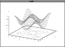

Figure 2.2: The gnuplot window and the postscript produced by gnuplot Chapter 3 Maple I
3.1 The simplification principle
Just as Reduce, Maple is an input-output machine. But, as main difference to Reduce, Maple will not automatically reformulate any input obeying some rules. Instead, Maple only executes explicit commands in the input but cites expressions without commands verbally. Hence, the simplification performance of Maple is controlled with explicit commands only - not with automatic reformulation rules. This nature of Maple might stem from its origin: Maple is programmed in C and the command syntax is strongly influenced by this language. There exist no rules or switches, Maple becomes active only when a command or an operator is called.
Maple offers a variety of commands to reformulate expressions. Most important though is one command, simplify, which tries to apply many different simplification methods to the expression and can be controlled with some options. For example, Maple will simply cite an input (x**2-1)/(x+1); as
but the answer on simplify((x**2-1)/(x+1)); is
The general syntax of simplify is
simplify (expr [,simplification_methods] [,assume=assumptions] );
Without specifying the simplification methods, simplify applies all methods. The parameter simplification_methods can be the name of a user-defined simplification procedure ‘simplify/name‘ (expr) or any of the build-in methods
BesselI, BesselJ, BesselK, BesselY, D, Ei, GAMMA, RootOf, LambertW, dilog, exp, ln, sqrt, polylog, pochhammer, trig (for trig functions), hypergeom (for hypergeometrics), radical (occurrence of fractional powers), power (occurrence of powers), exp, ln, and atsign (”@” - for operators)
One main problem with Maple’s simplification principle is, that simplify can not handle unknown (e.g. package-defined or user-defined) objects as expressions. For a tensor, e.g., the simplification command has to be applied on each component separately. Here, Reduce is clearly more elegant.
3.2 The interface
When you start a graphical version of Maple (’xmaple’) you are offered a worksheet displaying the first prompt > . Behind the prompt, Maple expects a command consisting out of an statement and a terminator (; or :). Again, the terminator decides whether Maple’s response is displayed (;) or not (:). Note that Maple is case sensitive! All examples displayed in this chapter are collected in the file examples.mws at [5]. The LaTeX code to display the examples here was produced by Maple (see Import / export).
Simplifying
(x**2-1)/(x+1);
simplify((x**2-1)/(x+1));
expand((x+y)**3);
A:=[(x^2-1)/(x+1),0];simplify(A);
A:=[0,0];simplify(A);
A:=array([[(x**2-1)/(x+1),0],[0,0]]); simplify(A);
A:=array([[0,0],[0,0]]); simplify(A);
Note that Maple makes an error in the last line because it does not handle arrays correctly! The operator % has the value of the last response of Maple (cf. ws in Reduce), i.e. in our case . Similar, %% and %%% represent the second and third last responses of Maple.
Usually, after typing the terminator one presses ENTER to execute the command. However, Maple offers to group commands in one so-called execution groups. To insert a line feed in this group one presses SHIFT+ENTER. Pressing ENTER somewhere in an execution group then executes all commands in this group.
3.3 User definitions
3.3.1 Names and assignments
Assignments
my_name123:=int(f(x),x);
‘$& "’ *@#!‘:=int(g(x),x);
my_name123:=’my_name123’;
‘$& "’ *@#!‘ := ’‘$& "’ *@#!‘’;i:=0:j:=2:k:=1: A.i.j.k;
As in Reduce any string (which is not reserved or a keyword, see table 3.1) may be used as a name. If you want some unusual string to be a name, the string has to be embraced by back(!)-quotes, e.g. ‘123 string‘ can be used as a name. The . sign allows to append numbers to a name.
The assignment operator is name:=expr. As in Reduce, the lhs name is identified with the rhs expression. There are three methods to unassign a name x:
– First with x:=’x’;. The embracing by single quotes(!) means an unevaluation of the enclosed string. Hence, x:=’x’; means an assignment of the unevaluated string x back to x.
– Second with unassign(’x’);. The unassign command also needs an unevalued string as parameter.
– Third with restart; which, however, unassigns all names. This methods is most secure to free the memory resource maple allocated.constants Pi I infinity gamma Catalan true false internal variables Digits Order constants libname printlevel lasterror status keywords and by do done elif else end fi for from if in intersect local minus mod not od option options or proc quit read save stop then to union while Table 3.1: Reserved names in Maple. As in Reduce it is important to distinguish between the expression assigned to a name and the value that Maple displays when evaluating the name. The following example shows the importance of the reassignment a:=a:. See also section 1.3.1.
a:=b: a;
b:=1: a;
a:=a:b:=2: a;
a:=’a’;
b:=’b’;3.3.2 Aliases
Aliases
alias(I=’I’):macro(I=’I’): 2*I; sqrt(-4);
macro(I=sqrt(-1)): 2*I; sqrt(-4);
macro(I=’I’): 2*I; sqrt(-4);
alias(I=sqrt(-1)): 2*I; sqrt(-4);
alias(I=’I’): 2*I; sqrt(-4);
Maple has two possibilities to define aliases which are quite useful (in contrast to the define command in Reduce). The first is macro and the second is alias. They have the same syntax but they have different meaning:
The macro(name=expr); command does not evaluate the expression expr before assigning it to the macro’s name. Whenever this name will appear in a future expression the first thing Maple does is to replace it by the associated value expr. However, Maple will not replace expr by the macro name in outputs. The point of a macro is to introduce shorthand notations for the input.
The alias(name=expr); command evaluates the expression expr before assigning it to the name. The value of expr cannot be a number. The effect of an alias is first, that Maple replaces all aliases by its value before evaluating expressions (as it does with macros), but second, that Maple also replaces expressions in the output by its alias if these exists one. So, the main point of an alias is introduce abbreviations in the input and output. The best example: The complex unit I is defined in Maple via: alias(I=sqrt(-1));
Macros and aliases can be changed and can be unassigned by assigning them back to their names: macro(name=name); and alias(name=name);
3.3.3 Substitutions and assumptions
Substitutions
f:=cos(x): x:=0: f; x:=’x’:
f:=cos(x): simplify(subs(x=0,f));
f:=’f’:
As in Reduce, one way to substitute identities in expressions is to make a local definition that represents the identity and let Maple reevaluate the expression. After this, f is still assigned to cos(x) but was evaluated to be 1. However, one should clear the assignment for x again with x:=’x’:. A more elegant way to substitute is the subs command the syntax of which is:
subs(eqn_list,expr);
Eventually, one has to simplify again to take the substitution into account.
Maple has one quite surprising and useful tool that Reduce lacks. Maple allows to make assumptions on unassigned names! With this, e.g., Maple simplifies to if one assumed before:
Assumptions
sqrt(x^2);
assume(x>0): about(x);
X
Originally x, renamed x~:
X
is assumed to be: RealRange(Open(0),infinity)
sqrt(x^2);
x := ’x’;
sqrt(x^2);
The syntax is assume(properties); The twiddle ~ behind the name x indicates that there are properties assumed for x. You can ask for properties of names with about and is and add more properties with additionally. Properties are deleted with the reassignment x:=’x’;
3.3.4 Operators
Operators
define(log2,log2(2)=1):
log2(2)*log2(3);define(fac,fac(0)=1,fac(n::posint)=n*fac(n-1)):
fac(5);unassign(log2,fac):
Maple offers the define commands to declare new operators. The general syntax is
define (name,properties);
definemore (name,properties);Here, properties are equations (rules) or any of the following key properties: linear, multilinear, orderless, flat (means associative). Note that it is possible to specify the type (see sections 4.2.2 and 4.2.3) of a parameter (e.g. n::posint to allow only positive integers for the parameter n). The command definemore adds more properties to an already defined operator.
3.3.5 Functionals
f(x):=cos(x): f(x); f(0); f(y);
f(x):=’f(x)’:
Functionals
g := x -> cos(x); g(x); g(0); g(y); D(g);
h := (x,y) -> sin(x)*sin(y); D[1](h); D[2](h);
k := h @ (x -> (x,exp(x))); k(x);
sin@exp; (sin@exp)(x); D(sin@exp); (D(sin@exp)) (x);
sin@@3; (sin@@3)(x);
g:=’g’: f:=’f’: h:=’h’: k:=’k’:
3.4 Solving
Maple offers the solve command for solving equations. The syntax is
solve (eqn_list,name_list);
For solving differential equations, use dsolve. For purely floating-point solutions use fsolve. Use isolve to solve for integer solutions, msolve to solve modulo a prime; rsolve for recurrences, and linalg[linsolve] to solve matrix equations.
Solving
solve(x^4-5*x^2+6*x=2,x);
diff(y(x),x)-y(x)^2+y(x)*sin(x)-cos(x); dsolve(%);
diff(x(t),t)=y(t); diff(y(t),t)=x(t)+y(t); x(0)=2,y(0)=1;
res := dsolve({%%%,%%,%},{x(t),y(t)}, type=numeric, output=procedurelist);
res(1);
We see how to plot solutions (esp. of dsolve) in chapter 4.
3.5 Commands and references
Maple has many, many command - a lot more than Reduce. Here, I only tried to collect the most basic ones in table 3.2. Other than Reduce, Maple offers complete commands for almost any standard problem instead of providing only elementary commands that suffice to write procedures. Many of them might provide quick help. Unfortunately, this means a vast number of commands which can hardly be overviewed. Most of these one will never use anyway because they are too specialized.
system control restart % %% %%% quit; # comment; with (package);
readlib (command_name); interface print[f]assignment name := expr; alias macro (name=expr); assume (properties); unassignment unassign (name); x:=’x’; substitution subs asubs (eqn_list,expr); subsop (eqn_list,expr); elementary expr + - * / ** expr; factorial (integer); expr mod integer; logical expr < <= <> = > >= expr; boolean and not or boolean; composition functional @ functional; functional @@ power; operators define (name,properties); selection op ([operand_number,]expr); denom numer (expr);
lhs rhs (eqn); collect [t]coeff[s]sets/lists { set_elements }; [ list_elements ]; seq (expr,range);
expr $ range; set intersect minus union set;
member map selectarrays array (ranges,component_list); evalm (matrix_expression); &* &*() loops (for from by [to|while] do od) (for in do od) (while do od) break next conditions (if then elif else fi) procedures (proc local global options end)
ERROR WARNING (message); RETURN (exprs);input output latex fortran C (expr); writeto appendto ("filename");
save names,"filename"; read "filename";
readdata("filename" [,format]); writedata("filename",list);
fopen fprintf fscanf fcloseplotting plot display odeplot textplot plotsetup interface evaluation E/eval eval[a|gf|m|b|c|hf|f|r] value allvalues expr; solving solve [i|m|r|f|d]solve (eqn_list,name_list); testeq (eqn); handing types whattype (expr); type convert (expr,type); Table 3.2: Elementary commands in Maple. We do not display the syntax of all commands and the innumerous functional operators sin etc. For explanations see table 1.2. The slash in E/eval means that there exist both commands Eval and eval, the first of which is the inert version (non-executing) whereas the second tries to execute the operation. The construction eval[a|gf|m|..] means that there exists evala evalgf evalm etc. Because of these innumerable commands Maple offers the most efficient way to work with Maple is by using the build-in help browser. This browser is opened via the programs menu or, more efficiently, by positioning the cursor on a word and pressing ’Crtl+F1’. To begin with, it is useful to have a look on the ’Index…’ topic (you find in the upper left window). There you find lists of expressions, functions, packages, etc. Alternatively, the ’Topic search…’ in the ’Help’ menu it useful to search for commands etc. alphabetically.
There is also online help in the internet available at [8]. This page is the producers address. You can find more addresses at [5].
There is also help available with in the non-graphical interface. The command ?subject will display help and examples for the specified subject. Also the commands index info usage example related (subject); provide help on the subject.
Integration / differentiation /dependencies:
diff(cos(5*x),x);
int(sin(x)**2,x);diff(f(x),x); diff(f,x); int(f(x),x); int(f,x);
f(x):=cos(x): f(x); f(0); f(y);
f(x):=’f(x)’:
Procedures
my_factorial:=proc(k)
local x,l: x:=1:
for l from 1 to k do x:=x*l: od:
end;my_factorial(16);
unassign(my_factorial):
Selection, sets, lists
op( int(f(x),x) ); op( [1,2,3] );
lhs(x=1); rhs(f(x)=sin(x));
{2,1}; [2,1];
seq( x[i], i=1..5 ); x[i] $ i=1..5;
{1,2} union {3,4}; {1,2} intersect {1,3};
f := x -> x**2:
map(f,[x,y]); map(f,x+(y*z)); map(f,x*(y+z));Logical operators
(x>3) and (y<=1);
subs({x=5,y=0},%);
eval(%);
Inert operators
Sum(1/2^i,i=1..k) = sum(1/2^i,i=1..k);
Limit(Sum(1/2^i,i=1..k),k=infinity) =
limit(sum(1/2^i,i=1..k),k=infinity);value(Limit(Sum(1/2^i,i=1..k),k=infinity));
Float evaluation
evalf(Pi,70);
Matrices
with(linalg): A:=matrix([[1,2,4],[2,1,2],[4,2,1]]);
X
Warning, new definition for norm
X
Warning, new definition for trace
det(A);
inverse(A);
$Chapter 4 Maple II
4.1 Examples
4.1.1 Generating a Julia set
# file "julia.map"

restart:

julia:=proc(c,s,file)
  local x,y,z,i,l:
  l:=[]:z:=0:
  for x from -3/2*s to 3/2*s do print(x): for y from -3/2*s to 3/2*s do
    z:=x/s+I*y/s:
    for i from 0 while i<100 and abs(Re(z))<2 and abs(Im(z))<2 do z:=z**2+c: od:
    if i=100 then l:=[op(l),[x,y]]: fi:
  od:od:

  save l,file:
end:

time(julia(0.3-0.5*I,200,"l6.map"));

with(plots):
read "l6.map":
plotsetup(ps,plotoutput="julia3.ps",plotoptions="noborder"):
listplot(l,style=POINT,axes=NONE,symbol=POINT,scaling=CONSTRAINED);
plotsetup(default):
Figure 4.1: The Julia set for . (File julia3.ps). 4.2 Advanced structures
4.2.1 Loops and conditions
The syntax for loop and conditional commands are
if boolean then statements [elif boolean then statements] [else statements] fi;
for name from start [by step] to stop do statements od;
for name from start [by step] while boolean do statements od;
for name in list do statements od;
while boolean do statements od;4.2.2 Procedures
The syntax for defining procedures in Maple is
name := proc (parameters[::types]) local names; global names; statements end;
The last of the statements needs no terminator and its value is automatically the return value of the procedure. One can specify the type of each parameter by adding ::type to the parameters name. Example:
f := proc(n::integer) factorial(n) end;
only excepts integers as parameters. Error messages or warnings can be produced with ERROR and WARNING. To use other procedures within a procedure it is sometimes useful to catch their error messages to prevent the procedure to be aborted. This is done be using the traperror command.
4.2.3 Types
There are innumerous different types defined in Maple. The main point of these is that procedures and operators (also user defined ones) can check if the given parameters have the correct type and throw error messages if not. E.g., if you pass an integer to the display command display(5); it says:
Error, (in display) invalid argument, 5, must be a plot structure, or a list/set/array thereof
This error message if quite useful. Also, if you want to tinker plot structures yourself and pass them to display, it is of course useful to find the exact description/syntax of the plot type in Maple’s help page plot, structure. With this knowledge you could also manipulate plots.
The commands
whattype(expr);
type(expr,type);
convert(expr,type);query the type of expr, check if expr has the type type, and convert expr such as to have the type type, respectively. See the help for the type for a list of all types Maple provides.
4.3 Export / import
For export and import there are four groups of commands. The first is very useful to store expressions. They are:
save names,"filename";
read "filename";Example:
f:=diff(sin(x),x);
save f,"sample.mai";
restart;
read "sample.mai";Here, the save command produces the file sample.mai which simply reads:
f := cos(x);
The following restart clears all assignments and cleans the memory buffer. The read command read the file as if it were typed in.
The second group of commands is similar to the out command in Reduce and only write into files. The commands are
writeto("filename");
appendto("filename");
writeto(terminal);They send all Maple’s output to the specified file. writeto(terminal); closes the file and redirects the output to the worksheet.
The third group of commands allows to read and write ordinary ascii data sheets as. Lists are used as buffer of such files:
readdata("filename" [, format_list] [, size_of_one_data_tuple]);
writedata("filename", list);readdata returns the data as list. The format_list can, e.g., be [integer,float,integer] for producing 3-tuples of data.
The fourth group of commands implements the syntax of the programming language C. They are
f := fopen("filename",READ|WRITE|APPEND,TEXT|BINARY);
fprintf(f,structure_string,exprs);
fscanf(f,structure_string,variables);
fclose(f);The meaning should be clear if one knows C. The commands feof, fflush, fremove, filepos also belong to this group. With these commands you can produce files with arbitrary content.
4.3.1 LaTeX, Fortran, and C
The commands latex(expr), fortran(expr), and C(expr) are nice facilities to export to LaTeX, Fortran of the programming language C. See these examples:
> restart: readlib(C):

> latex(Limit(Sum(1/2^i,i=1..k),k=infinity));
lim _{k\rightarrow \infty }\sum _{i=1}^{k}\left ({2}^{i}\right )^{-1}


> f:= x -> Pi*ln(x^2)-sqrt(2)*ln(x^2)^2;

> C(f,optimized);
/* The options were    : operatorarrow */
#include <math.h>
double f(x)
double x;
{
  double t2;
  double t1;
  double t4;
  double t5;
  {
    t1 = x*x;
    t2 = log(t1);
    t4 = sqrt(2.0);
    t5 = t2*t2;
    return(0.3141592653589793E1*t2-t4*t5);
  }
}

> fastgrow:=proc(k)
>   local x,i;
>   x:=1;
>   for i from 1 to k do x:=x+x**x; od;
>   x;
> end;

> fortran(fastgrow);
      real function fastgrow(k)
      real k

      integer i
      real x

        x = 1
        do 1000 i = 1,k,1
          x = x+x**x
1000    continue
        fastgrow = x
        return
      end
A possibility to export whole Maple worksheet to Latex is with the menu File – Export As – LaTeX. I used this method in this paper. This will produce a LaTeX document reproducing the appearance of the worksheet. The Maple style files have to be installed for this. One can get them at
http://www.maplesoft.com/latex_patch.html
and provisionally copy them in the same directory as the LaTeX file.4.3.2 Plotting
Again, Maple offers innumerous commands to generate plots. Here, I present only those that I find most elementary:
plot(function_list [,horizontal_range] [,vertical_range] [,plot_options]);
textplot({[x_coord,y_coord,"text"],..} [,plot_options]);
display(plot_structure_list [,plot_options]);
with(plots);
odeplot(numeric_dsolve_output,function_list,x_range [,plot_options]);
plotsetup(device_type [,options]);For handling plots it is important to realize that all plot commands return a plot structure of type PLOT. See this example:
plt:=plot(sin(x),x=-Pi..Pi):
save plt,"sample.plt":
restart:
read "sample.plt":
display(plt);
Here, we assign the plot of to the variable plt and store this variable in the sample.plt file. This is very useful when it takes long to produce plots (e.g. with odeplot!). The following commands produce the postscript in figure 4.2 and write it in the file mapplot.ps.
with(plots):
solution := dsolve({ diff(y(x),x) = sin(x*y(x)),y(0)=2},y(x),type=numeric):
plt := odeplot(solution,[x,y(x)],0..6,labels=[x,y],labelfont=[TIMES,ITALIC,22]):
txt := textplot([2.5,2.5,"Solution of y’=sin(x*y), y(0)=2"],align=RIGHT,font=[TIMES,ROMAN,22]):
plotsetup(ps,plotoutput="mapplot.ps",plotoptions="noborder"):
display({plt,txt},axesfont=[TIMES,ROMAN,18]);
plotsetup(default):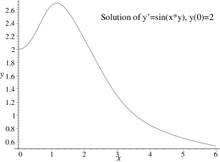
Figure 4.2: Plot produced by Maple Chapter 5 Tensor type calculi on Reduce and Maple
5.1 Maple
5.1.1 The tensor package
Maple provides a the tensor package to implement the tensor calculus. This package is strongly oriented to perform the standard calculations in Einsteinian gravity, i.e. to calculate the Christoffel symbol, the Riemannian curvature tensor, the Ricci tensor, etc. from a given symmetric metric. For this special purpose the package is quite useful. Of course, the package provides also elementary operations to work with tensors: adding tensors lin_com, the tensor product prod, raising, lowering, contracting, and (anti-) symmetrizing indices raise, lower, contract, antisymmetrize, symmetrize. However, as one can see from table 5.1, the syntax of these commands is not at all in analogy to the usual notation of tensor calculus: To setup a general 3rd rank tensor in 2D space with two covariant and one contravariant indices one has to declare
restart:with(tensor):
A:=create([-1,-1,1],array(
  [[[a.1.1.1(x.1,x.2),a.1.1.2(x.1,x.2)],[a.1.2.1(x.1,x.2),a.1.2.2(x.1,x.2)]],
   [[a.2.1.1(x.1,x.2),a.2.1.2(x.1,x.2)],[a.2.2.1(x.1,x.2),a.2.2.2(x.1,x.2)]]]
));
To specify the tensor type, ’-1’ means a covariant index whereas ’1’ means a contravariant (in contrast to what is said in the help page of create). Maple starts counting indices from 1. As you see, one has to introduce general names for all components oneself (that include the dependency on coordinates). The following examples show other tensor manipulations:
usual notation tensor package syntax lin_com(5,A,B,2,c); prod(A,B,[1,3]); contract(A,[1,3]); partial_diff(A,[x.1,x.2,x.3,x.4]); In contrast, we will see the Excalc allows tensor manipulations that are a direct mirror of the usual notation. The entermetric command allows to enter a metric interactively. Personally, I find this unacceptable for a CA system.
declarations create (tensor_type,components_array); entermetric elementary ops lin_com (coefficiants_and_tensors);
prod (1st_tensor,2nd_tensor,index_pairs_to_contract);
raise lower (metric,tensor,indices);
contract (tensor,index_pairs);
symmetrize antisymmetrize (tensor,index_array);
get_compts get_char get_rank (tensor);differentiation partial_diff exterior_diff (tensor,coord_array);
cov_diff (tensor,coord_array,Christoffel_symbol);
Lie_diff directional_diff (tensor,vector,coord_array);more ops compare invert dual permute_indices exterior_prod act conj frame commutator certain tensors Levi_Civita d1metric d2metric coord trans Jacobian change_basis transform GR tensors tensorsGR display_allGR displayGR Christoffel1 Christoffel2 Einstein Ricci Ricciscalar Riemann Weyl connexF RiemannF invars petrov Newmann-P. convertNP npcurve npspin extract eqns Killing_eqns geodesic_eqns Table 5.1: The commands of Maple’s tensor package. The syntax is only specified for elementary commands. Finally, we show how simple it is to calculate the standard GR tensors with the tensor package for a given metric. In the example we derive the Schwarzschild metric as solution of the Einstein equation for a general static, spherically symmetric ansatz.
restart:with(tensor):
gdd:=create([-1,-1],array(symmetric,[
[f(r),0,0,0],
[0,-g(r)/f(r),0,0],
[0,0,-r^2,0],
[0,0,0,-r^2*sin(theta)^2]
]));tensorsGR([t,r,theta,phi],gdd,
guu,gdet,chris1,chris2,riem,ric,ric_scalar,einstein,weyl):eqs:=get_compts(ric);
dsolve({eqs[1,1],eqs[2,2]},{f(r),g(r)});
5.1.2 The GRTensor package
restart:
read "/home/mt/usr/maple/lib5/grii.m":
grtensor():makeg(ss):
Makeg 2.0: GRTensor metric/basis entry utility

To quit makeg, type ’exit’ at any prompt.{\large }

Do you wish to enter a 1) metric [g(dn,dn)],
                       2) line element [ds],
                       3) non-holonomic basis [e(1)...e(n)], or
                       4) NP tetrad [l,n,m,mbar]?
2:
Enter coordinates as a LIST (e.g. [r,theta,phi,t]):
[t,r,theta,phi]:
Enter the line element using d[coord] to indicate differentials.
(for example,  r^2*(d[theta]^2 + sin(theta)^2*d[phi]^2)
[Type ’exit’ to quit makeg]
 ds^2 =
f(r)*d[t]^2 - g(r)/f(r)*d[r]^2 - r^2*(d[theta]^2 + sin(theta)^2 *
d[phi]^2):If there are any complex valued coordinates, constants or functions for this spacetime, please enter them as a SET ( eg. { z, psi } ).Complex quantities [default={}]:{}:
You may choose to 0) Use the metric WITHOUT saving it,
                  1) Save the metric as it is,
                  2) Correct an element of the metric,
                  3) Re-enter the metric,
                  4) Add/change constraint equations,
                  5) Add a text description, or
                  6) Abandon this metric and return to Maple.
0:
Calculated ds for ss (.020000 sec.)
makeg() completed.
grcalc( R(dn,dn) ):
Calculated detg for ss (.010000 sec.)
Calculated g(up,up) for ss (.020000 sec.)
Calculated g(dn,dn,pdn) for ss (.020000 sec.)
Calculated Chr(dn,dn,dn) for ss (.020000 sec.)
Calculated Chr(dn,dn,up) for ss (.040000 sec.)
Calculated R(dn,dn) for ss (.040000 sec.)
grdisplay( R(dn,dn) ):
eqs:={grcomponent(R (dn,dn), [1,1]),grcomponent(R (dn,dn),
[2,2])}:dsolve(eqs,{f(r),g(r)});
restart: read "/files/home/part3/mt/usr/maple/lib5/grii.m": grtensor(): makeg(ss): 2: [t,r,theta,phi]: f(r)*d[t]^2 - g(r)/f(r)*d[r]^2 - r^2*(d[theta]^2 + sin(theta)^2 * d[phi]^2): {}: 0: grcalc( R(dn,dn) ): grdisplay( R(dn,dn) ): eqs:={grcomponent(R (dn,dn), [1,1]),grcomponent(R (dn,dn), [2,2])}: dsolve(eqs,{f(r),g(r)}): latex({%});5.2 Excalc
Who doubts about the beauty of the exterior calculus?! Reduce offers a package Excalc that provides very handy methods to handle exterior forms as well as tensors. Fortunately, this package implements elementary declarations and operators that let all freedom to the user to define quantities - it does not offer complete GR routines as the tensor of GRtensor packages in Maple that impose their notations and conventions. Excalc really generally implements the tensor and exterior calculus. Tensors can also be handled by Reduce without the Excalc package – you can find some explanation for this in the appendix. However, since with Excalc it is a lot easier and more beautiful, I advice to use the Excalc package to manipulate tensors.
The Excalc package is loaded with load_package excalc$. It provides the commands and operators summarized in table 5.2. The table should explain most commands. There is online help available at [7]. We now give more detailed explanations on the basic commands.
declare forms/tensors pform name[(tensor_indices)]=degree; declare vectors tvector names; declare dependence fdomain name=name(dependency); tensor symmetries index_symmetries tensor: [symmetric [in index_pairs]] [antisymmetric [in index_pairs]]; get form degree exdegree(form); exterior derivative d (form); partial differentiation @ (form,coord); inner product vector _| form; hodge dual # (form); Lie derivative vector |_ form; variational derivative vardf (form,non_tensor_form); declare coframe coframe coframe_def [with metric metric_def | with signature signature]; declare frame frame name; display coframe displayframe; indices indexrange numbers_or_names; set space dimension spacedim number; tangent vector @ (coord); epsilon tensor eps (indices); Christoffel symbol riemannconx name; others noether keep nosum renosum noxpnd forder remforder xpnd Table 5.2: The commands of Excalc. A form is in general an exterior form declared with pform which can have tensor indices also. For the meaning of index_pairs, coframe_def, metric_def, and signature see the text. The most important declaration is pform which allows to introduce exterior forms with additional tensor indices. E.g., with the following we introduce a 2rd rank tensor t (), a 4th rank tensor r (), and a 2-form p with one index ():
pform t(i,j)=0,r(i,j,k,l)=0,p(i)=2$
After this declaration, these tensors/forms can be refered to by t(1st_index_name,2nd_index_name), etc., i.e. we can use arbitrary names for the indices. Specifying the index range lets Excalc run the index names over this range in all expression.
Putting a minus sign in front of the index name lowers the index, without a minus sign the index is a contravariant index. Excalc knows the summation convention summing over identical lower and upper tensor indices. E.g., the following examples calculate the trace and perform the assignment :
1: load_package excalc$
*** ^ redefined

2: pform t(i,j)=0,r(i,j,k,l)=0,p(i)=2$

3: t(-i,i);

   i
t
 i

4: t(i,j):=r(-k,i,j,k);

 i j       i j k
t    := r
         k

5: indexrange 0,1,y,z$

6: t(-i,i);

   0      1      y      z
t    + t    + t    + t
 0      1      y      z

7: t(0,0):=a$ t(0,0);

a

9: t (-0,0);

   0
t
 0
If we have defined a metric Excalc automatically calculates the (contra-)covariant components from assignments to (co-)contravariant components. For a diagonal metric, the response to input 9 would then be . Specifying the metric structure is a little bit involved. Roughly, the syntax to introduce a frame and metric is
coframe coframe_def [with metric metric_def | with signature signature];
The following examples should make clear what the parameters mean:
% file "exc1"
load_package excalc$

% symbolic 3D coframe with Euclidean metric:
coframe o(0),o(1),o(2)$

% polar coframe with Euclidean metric:
coframe o(r)=d r,o(p)=r * d phi$

% Schwarzschild metric in anholonomic/diagonalized form:
coframe o(0)=f * d t,
        o(1)=1/f * d r,
        o(2)=r * d theta,
        o(3)=r*sin(theta) * d phi
with signature (+1,-1,-1,-1)$

% symbolic 4D coframe with arbitrary metric:
operator gll,o$         % introduce general notations
for i:=0:3 do for j:=i+1:3 do gll(i,j):=gll(j,i)$     % symmetrize metric
let { metric_def => for i:=0:3 sum for j:=0:3 sum gll(i,j)*o(i)*o(j) };
coframe o(0),o(1),o(2),o(3) with metric g = metric_def$

% holonomic 4D coframe with arbitrary metric and coordinates x(a):
operator gll,o$
for i:=0:3 do for j:=i+1:3 do gll(i,j):=gll(j,i)$
let { metric_def => for i:=0:3 sum for j:=0:3 sum gll(i,j)*o(i)*o(j) };
coframe o(0)=d x0,o(1)=d x1,o(2)=d x2,o(3)=d x3 with metric g = metric_def$
pform x(i)=0$           % introduce coordinates as indexed 0-form defined as:
x(-0):=x0$ x(-1):=x1$ x(-2):=x2$ x(-3):=x3$
frame e$                % generate a frame e(-a) dual to o(a)
e(-a) _| o(-b);         %-> gll(a,b)
The first example introduces a coframe index by indices running over in the Euclidean (because no metric is specified) 3D space. The second example introduces alphabetic(!) indices running over and defines the anhonomic coframe with respect to holonomic coordinate derivatives (,). Thus, also r and phi are introduces as coordinates (e.g. enabling to write @ r for the radial vector). The 3rd example introduces the Schwarzschild geometry with diagonal metric and anholonomic coframe.
The 4th example introduces a general coframe with arbitrary metric. The metric (low-low) components have been predefined as symmetric operator. Since the coframe command does not accept for constructions, the variable metric_def was used as alias for the metric expression. It is better to use let rules to predefine expressions that will be used in the coframe definition. The 5th example introduces a holonomic coframe with arbitrary metric, coordinate basis x(i), and holonomic frame @ x(a) which coincides with e(-a).
The command
frame e$
introduces the name e for the respective frame (defined via the metric by or ). Thus, the last example of the coframe definitions will yield
e(-a) _| o(-b) \% throws gll(a,b)
Specifying the symmetries of tensors (or tensor indices on forms) saves Reduce from calculating redundant components and thus saves time. Excalc provides the index_symmetries command for this. Note that if no metric is specified before the index_symmetries command assumes an Euclidean metric! The syntax given in the table is
index_symmetries tensor: [symmetric [in index_pairs]] [antisymmetric [in index_pairs]];
Here, index_pairs can be {i,j} etc. but also pairs of pairs of indices, i.e. {{i,j},{k,l}} which means that the pair {i,j} (anti-)commutes with the pair {k,l}. The following example will clarify this:
index_symmetries t(i,j): symmetric$
index_symmetries r(k,l,m,n): symmetric in {k,l},{m,n} antisymmetric in {{k,l},{m,n}}$
These commands mean and .
The rest of the commands works rather canonical and can be understood by looking at some examples: The first example implements the Schwarzschild metric in the tensor calculus:
% file "exc2"
% The Schwarzschild metric in tensor formalism

load_package excalc$

% introducing the metric (the symbolic coframe is of no importance):
depend(f,r)$ depend(g,r)$
coframe o(0),o(1),o(2),o(3) with metric
g = f**2*o(0)**2 -g**2/f**2*o(1)**2 -r**2*o(2)**2 -r**2*sin(theta)**2*o(3)**2$

% introducing coordinates with running indices:
pform x(i)=0$
x(-0):=t$ x(-1):=r$ x(-2):=theta$ x(-3):=phi$

% calculating the Christoffel symbol:
pform chris(i,j,k)=0$
index_symmetries chris(i,j,k): symmetric in {i,j}$
chris(-i,-j,-k) :=
  (1/2)* (@(g(-j,-k),x(-i)) + @(g(-k,-i),x(-j)) - @(g(-i,-j),x(-k)))$

% the Riemannian curvature:
pform riem(i,j,k,l)=0$
index_symmetries riem(i,j,k,l): antisymmetric in {i,j},{k,l}
                                symmetric in {{i,j},{k,l}}$
riem(-i,-j,-k,l):=
     @(chris(-j,-k,l),x(-i)) + chris(-i,-m,l)*chris(-j,-k,m)
   - @(chris(-i,-k,l),x(-j)) - chris(-j,-m,l)*chris(-i,-k,m)$

% the Ricci tensor:
pform ric(i,j)=0$
index_symmetries ric(i,j): symmetric$
ric(-i,-j) := riem(-m,-i,-j,m)$

% the Ricci scalar:
pform ricscalar=0$
ricscalar := ric(-i,i);

let {g=>1,f=>sqrt(1-mm/r)}$
ric(-i,-j);

end$
The next example proves the Bianchi identity in a purely symbolic manner:
% file "exc3"
% Proving the Bianchi identity in the exterior calculus
%
load_package excalc$

indexrange 0,1,2,3$

% general introduction of a connection:
pform gamma(a,b)=1$

% definition of the curvature:
pform curv(a,b)=2$
curv(-a,b):=d gamma(-a,b) - gamma(-a,c) ^ gamma(-c,b)$

% Bianchi identity:
d curv(-a,b) - gamma(-a,c) ^ curv(-c,b) + gamma(-c,b) ^ curv(-a,c);
  %-> yields zero!

end$
The next example implements the Taub-NUT solution with electric charge in the exterior calculus (in the Kaluza-Klein formalism):
% nut.exi, Marc Toussaint, Cologne
% 99-Oct-19
%
% The Taub-NUT solution with electric charge

load_package excalc$
off gcd,exp$

% COFRAME %%%%%%%%%%%%%%%%%%%%%%%%%%%%%%%%%%%%%%%%%%%%%%%%%%%%%%%%%%%%%%%%%%%%%

clear t,r,theta,phi,o,e,f,rho,dtau,dsigma,m,n,q$

pform f=0,rho=0$
fdomain f=f(r),rho=rho(r)$
let { dtau   => d t - 2*n*cos(theta)*d phi,
      dsigma => (r**2+n**2)*d phi }$

dim:=5$
coframe o(0) = f/rho* dtau,
        o(1) = rho/f* d r,
        o(2) =  rho * d theta,
        o(3) = 1/rho*sin(theta)* dsigma,
        o(5) = d w + r/rho**2* q*dtau
with signature (1,-1,-1,-1,-1)$
frame e$


% ANSATZ %%%%%%%%%%%%%%%%%%%%%%%%%%%%%%%%%%%%%%%%%%%%%%%%%%%%%%%%%%%%%%%%%%%%%%

f    := sqrt(r**2-2*r*m-n**2+q**2/4)$
rho  := sqrt(r**2+n**2)$


% FIELD EQUATION %%%%%%%%%%%%%%%%%%%%%%%%%%%%%%%%%%%%%%%%%%%%%%%%%%%%%%%%%%%%%%

% Christoffel symbol:
        pform chris1(a,b)=1$
        Riemannconx chris1$
        chris1(a,b):=chris1(b,a)$

% Riemannian curvature and Einstein 3-form:
        pform rie2(a,b)=2,einstein3(a)=dim-1$
        rie2(-a,b):=d chris1(-a,b) + chris1(-c,b)^chris1(-a,c)$
        einstein3(a):=1/2*#(o(a)^o(b)^o(c)) ^ rie2(-b,-c)$

% Result:
        einstein3(a);   %-> zero (except the (5,5)-compopnent)

end;
5.3 The tensor calculus in Reduce
The tensor calculus is realized in Reduce by manipulating arrays with elementary commands. Usually, the first step is to introduce countable (i.e. indexed) coordinates as an operator (giving the coordinate for each index). Next one can introduce a metric and calculate the inverse to be able to raise and lower indices. Then tensors are introduced as arrays and all operations are performed by explicitly running over the indices (with the for command). Whether the array contains covariant or contravariant components is specified by adding the characters ’l’ for lower and ’u’ for upper indices to the name. The following example will follow this scheme to calculate the curvature of a general static, symmetric geometry in polar coordinates and thereby derive the Schwarzschild metric.
% indexed polar coordinates:
operator x$
x(0):=t$ x(1):=r$ x(2):=theta$ x(3):=phi$

% the metric (gll) with two lower and its inverse (guu) with two upper indices:
array gll(3,3),guu(3,3)$            % arrays are initialized with zero

% static, spherically symmetric ansatz, signature: + - - - :
depend(f,r)$
depend(g,r)$
gll(0,0):=f**2$ gll(1,1):=- g**2/f**2$ gll(2,2):=-r**2$ gll(3,3):=-r**2*(sin(theta))**2$

% calculating the inverse by using Reduce’s matrix calculus:
matrix m(4,4)$
for i:=0:3 do for j:=i:3 do m(j+1,i+1):=m(i+1,j+1):=gll(i,j)$
m:=1/m$                         % calculates the inverse
for i:=0:3 do for j:=i:3 do guu(j,i):=guu(i,j):=m(i+1,j+1)$
clear m$

% calculating the Christoffel symbol of type low-low-low and low-low-up:
array chrislll(3,3,3),chrisllu(3,3,3)$
for i:=0:3 do for j:=i:3 do <<
  for k:=0:3 do chrislll(j,i,k) := chrislll(i,j,k) :=
    (1/2) * (df(gll(j,k),x(i)) + df(gll(k,i),x(j)) - df(gll(i,j),x(k)))$
  for k:=0:3 do chrisllu(j,i,k) := chrisllu(i,j,k) :=
    for m:=0:3 sum guu(k,m) * chrislll(i,j,m)$
>>$

% calculating the Riemannian curvature (neglecting symmetries -> inefficient!):
array riemlllu(3,3,3,3)$
for i:=0:3 do for j:=0:3 do for k:=0:3 do for l:=0:3 do
  riemlllu(i,j,k,l):=
    df(chrisllu(j,k,l),x(i)) - df(chrisllu(i,k,l),x(j))
    + for m:=0:3 sum (  chrisllu(i,m,l)*chrisllu(j,k,m)
                      - chrisllu(j,m,l)*chrisllu(i,k,m) )$

% the Ricci tensor:
array ricll(3,3)$
for i:=0:3 do for j:=0:3 do
  ricll(i,j) := for k:=0:3 sum riemlllu(k,i,j,k)$

% the Ricci scalar:
ricscalar := for k:=0:3 sum for l:=0:3 sum guu(l,k)*ricll(k,l)$

{ricll(0,0),ricll(1,1),ricll(2,2),ricll(3,3)} where {g=>1,f=>sqrt(1-mm/r)};
Bibliography
- [1] F.W. Hehl, V. Winkelmann, H. Meyer: Reduce: Ein Kompaktkurs über die Anwendung von Computer-Algebra. Springer, Berlin, 2. Auflage (1992).
- [2] G. Rayna: Reduce: Software for algebraic computation. Springer, Berlin (1987).
- [3] M. MacCallum, F. Wright: Algebraic computing with Reduce. Lecture notes from the 1st Brazil school on computer algebra. Clarendon Press, Oxford (1991).
- [4] D. Redfern: The Maple handbook. Maple V release 3. Springer, Berlin (1994).
-
[5]
Sources for these lectures:
http://www.thp.uni-koeln.de/~mt/work/1999mexico/ -
[6]
Reduce user’s manual:
http://www.uni-koeln.de/REDUCE/3.6/doc/reduce/ -
[7]
Excalc user’s manual:
http://www.uni-koeln.de/REDUCE/3.6/doc/excalc/excalc.html -
[8]
Maple’s homepage:
http://www.maplesoft.com/ -
[9]
ZIB, Berlin:
http://www.zib.de/Symbolik/reduce/moredocs/ -
[10]
The CATHODE project: homepage:
http://www-lmc.imag.fr/cathode2/, software page:http://www-sop.inria.fr/cafe/Manuel.Bronstein/cathode/software.html