Search in Power-Law Networks

Abstract

Many communication and social networks have power-law link distributions, containing a few nodes which have a very high degree and many with low degree. The high connectivity nodes play the important role of hubs in communication and networking, a fact which can be exploited when designing efficient search algorithms. We introduce a number of local search strategies which utilize high degree nodes in power-law graphs and which have costs which scale sub-linearly with the size of the graph. We also demonstrate the utility of these strategies on the Gnutella peer-to-peer network.

1 Introduction

A number of large distributed systems, ranging from social [13] to communication [11] to biological networks [9] display a power-law distribution in their node degree. This distribution reflects the existence of a few nodes with very high degree and many with low degree, a feature not found in standard random graphs [5]. An illustration of the power-law nature of such networks is given by the AT&T call graph. A call graph is a graph representation of telephone traffic on a given day in which nodes represent people and links the phone calls among them.

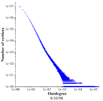
As is shown in Figure 1, the out-link degree distribution for a massive graph of telephone calls between individuals is power-law, with an exponent of approximately 2.1. The same distribution is obtained for the case of in-links. This power-law in the link distribution reflects the presence of central individuals who interact with many others on a daily basis and play a key role in relaying information.

While recent work has concentrated on the properties of these power-law networks and how they are dynamically generated [2, 8, 12], there remains the interesting problem of finding efficient algorithms for searching within these particular kinds of graphs. Recently, Kleinberg [10] studied search algorithms in a graph where nodes are placed on a 2-D lattice and each node has a fixed number of links whose placement is correlated with lattice distance to the other nodes. Under a specific form of the correlation, an algorithm with knowledge of the target’s location can find the target in polylogarithmic time.

In the most general distributed search context however, one may have very little information about the location of the target. Increasingly a number of pervasive electronic networks, both wired and wireless, make geographic location less relevant. A particularly interesting example is provided by the recent emergence of peer-to-peer networks, which have gained enormous popularity with users wanting to share their computer files. In such networks, the name of the target file may be known, but due to the network’s ad hoc nature, until a real-time search is performed the node holding the file is not known. In contrast to the scenario considered by Kleinberg, there is no global information about the position of the target, and hence it is not possible to determine whether a step is a move towards or away from the target. One simple way to locate files, implemented by Napster, is to use a central server which contains an index of all the files every node is sharing as they join the network. This is the equivalent of having a giant white pages for the entire United States. Such directories now exist online, and have in a sense reduced the need to find people by passing messages. But for various reasons, including privacy and copyright issues, in a peer-to-peer network it is not always desirable to have a central server.

File-sharing systems which do not have a central server include Gnutella and Freenet. Files are found by forwarding queries to one’s neighbors until the target is found. Recent measurements of Gnutella networks [3] and simulated Freenet networks [7] show that they have power-law degree distributions. In this paper, we propose a number of message-passing algorithms that can be efficiently used to search through power law networks such as Gnutella. Like the networks that they are designed for, these algorithms are completely decentralized and exploit the power law link distribution in the node degree. The algorithms use local information such as the identities and connectedness of their neighbors, and their neighbors’ neighbors, but not the target’s global position. We demonstrate that our search algorithms work well on real Gnutella networks, scale sub-linearly with the number of nodes, and may help reduce the network search traffic that tends to cripple such networks.

The paper is organized as follows. In Section 2, we present analytical results on message-passing in power-law graphs, followed by simulation results in Section 3. Section 4 compares the results with Poisson random graphs. In Section 5 we consider the application of our algorithms to Gnutella, and Section 6 concludes.

Figure 1: Out-degree distribution for the AT&T call graph.

2 Search in Power-Law Random Graphs

In this section we use the generating function formalism introduced by Newman [12] for graphs with arbitrary degree distributions to analytically characterize serach-cost scaling in power-law graphs.

2.1 Random Walk Search

Let $G_{0}(x)$ be the generating function for the distribution of the vertex degrees $k$. Then

$$G_{0}(x)=\sum_{0}^{\infty}p_{k}x^{k}$$ (1)

where $p_{k}$ is the probability that a randomly chosen vertex on the graph has degree $k$.

For a graph with a power-law distribution with exponent $\tau$, minimum degree $k=1$ and an abrupt cutoff at $m=k_{max}$, the generating function is given by

$$G_{0}(x)=c\sum_{1}^{m}k^{-\tau}x^{k}$$ (2)

with $c$ a normalization constant which depends on $m$ and $\tau$ to satisfy the normalization requirement

$$G_{0}(1)=c\sum_{1}^{m}k^{-\tau}=1$$ (3)

The average degree of a randomly chosen vertex is given by

$$<k>=\sum_{1}^{m}kp_{k}=G_{0}^{\prime}(1)$$ (4)

Note that the average degree of a vertex chosen at random and one arrived at by following a random edge are different. A random edge arrives at a vertex with probability proportional to the degree of the vertex, i.e. $p^{\prime}(k)\sim kp_{k}$. The correctly normalized distribution is given by

$$\frac{\sum_{k}kp_{k}x^{k}}{\sum_{k}kp_{k}}=x\frac{G^{\prime}_{0}(x)}{G^{\prime}_{0}(1)}$$ (5)

If we want to consider the number of outgoing edges from the vertex we arrived at, but not include the edge we just came on, we need to divide by one power of $x$. Hence the number of new neighbors encountered on each step of a random walk is given by the generating function

$$G_{1}(x)=\frac{G^{\prime}_{0}(x)}{G^{\prime}_{0}(1)}$$ (6)

where $G^{\prime}_{0}(1)$ is the average degree of a randomly chosen vertex as mentioned previously.

In real social networks it is reasonable that one one would have at least some knowledge of one’s friends’ friends. Hence, we now compute the distribution of second degree neighbors. The probability that any of the 2nd degree neighbors connect to any of the first degree neighbors or to one another goes as $N^{-1}$ and can be ignored in the limit of large $N$. Therefore, the distribution of the second neighbors of the original randomly chosen vertex is determined by

$$\sum_{k}p_{k}[G_{1}(x)]^{k}=G_{0}(G_{1}(x))$$ (7)

It follows that the average number of second degree neighbors is given by

$$z_{2A}=[\frac{\partial}{\partial x}G_{0}(G_{1}(x))]_{x=1}=G^{\prime}_{0}(1)G^{\prime}_{1}(1)$$ (8)

Similarly, if the original vertex was not chosen at random, but arrived at by following a random edge, then the number of second degree neighbors would be given by

$$z_{2B}=[\frac{\partial}{\partial x}G_{1}(G_{1}(x))]_{x=1}=[G^{\prime}_{1}(1)]^{2}$$ (9)

In both Equation 8 and Equation 9 the fact that $G_{1}(1)=1$ was used.

Both these expressions depend on the values $G^{\prime}_{0}(1)$ and $G^{\prime}_{1}(1)$ so let’s calculate those for given $\tau$ and $m$. For simplicity and relevance to most real-world networks of interest we assume $2<\tau<3$.

$$G^{\prime}_{0}(1)=\sum_{1}^{m}ck^{1-\tau}\sim\int_{1}^{m}x^{\tau-1}dx=\frac{1}{\tau-2}(1-m^{2-\tau})$$ (10)

$$G^{\prime}_{1}(1) = \frac{1}{G^{\prime}_{0}(1)}\frac{\partial}{\partial x}\sum_{1}^{m}ck^{1-\tau}x^{k-1}$$ (11)

$$= \frac{1}{G^{\prime}_{0}(1)}\sum_{2}^{m}ck^{1-\tau}(k-1)x^{k-2}$$ (13)

$$\sim \frac{1}{G^{\prime}_{0}(1)}(\frac{m^{3-\tau}(\tau-2)-2^{2-\tau}(\tau-1)+m^{2-\tau}(3-\tau)}{(\tau-2)(3-\tau)}$$ (14)

for large cutoff values $m$. Now we impose the cutoff of Aiello et al. [13] at $m\sim N^{1/\tau}$. Since $m$ scales with the size of the graph $N$ and for $2<\tau<3$ the exponent $2-\tau$ is negative, we can neglect terms constant in $m$. This leaves

$$G^{\prime}_{1}(1)\\ =\frac{1}{G^{\prime}_{0}(1)}\frac{m^{3-\tau}}{(3-\tau)}$$ (15)

Substituting into Equation 8 (the starting node is chosen at random) we obtain

$$z_{2A}=G^{\prime}_{0}(1)G^{\prime}_{1}(1)\sim m^{3-\tau}$$ (16)

We can also derive $z_{2B}$, the number of 2nd degree neighbors encountered as one is doing a random walk on the graph.

$$z_{2B}=[G^{\prime}_{1}(1)]^{2}=[\frac{\tau-2}{1-m^{2-\tau}}\frac{m^{3-\tau}}{3-\tau}]^{2}$$ (17)

Letting $m\sim N^{1/\tau}$ as above, we obtain

$$z_{2B}\sim N^{2(\frac{3}{\tau}-1)}$$ (18)

and the scaling of the number of steps required becomes

$$s\sim N^{3(1-2/\tau)}$$ (19)

In the limit $\tau\rightarrow 2$, equation 17 becomes

$$z_{2B}\sim\frac{N}{ln^{2}(N)}$$ (20)

and the scaling of the number of steps required is

$$s\sim ln^{2}(N)$$ (21)

2.2 Search utilizing high degree nodes

Random walks in power-law networks naturally gravitate towards the high degree nodes, but an even better scaling is achieved by intentionally choosing high degree nodes. For $\tau$ sufficiently close to $2$ one can walk down the degree sequence, visiting the node with the highest degree, followed by a node of the next highest degree, etc. Let $m-a$ be the degree of the last node we need to visit in order to scan a certain fraction of the graph. We make the self-consistent assumption that $a<<$m, i.e. the degree of the node hasn’t dropped too much by the time we have scanned a fraction of the graph. Then the number of first degree neighbors scanned is given by

$$z_{1D}=\int^{m}_{m-a}Nk^{1-\tau}dk\sim Nam^{1-\tau}$$ (22)

The number of nodes having degree between $m-a$ and $m$, or equivalently, the number of steps taken is given by $\int^{m}_{m-a}k^{-\tau}\sim a$. The number of second degree neighbors when one follows the degree sequence is given by:

$$z_{1D}\ast G^{\prime}_{1}(1)\sim Nam^{2(2-\tau)}$$ (23)

which gives the number of steps required as

$$s\sim m^{2(\tau-2)}\sim N^{2-\frac{4}{\tau}}$$ (24)

We now consider when and why it is possible to go down the degree sequence. We start with the fact that the original degree distribution is a power-law:

$$p(x)=(\sum_{1}^{m}x^{-\tau})^{-1}x^{-\tau}$$ (25)

where $m=N^{1/\tau}$ is the maximum degree. A node chosen by following a random link in the graph will have its remaining outgoing edges distributed according to

$$p^{\prime}(x)=(\sum_{0}^{m-1}(x+1)^{(1-\tau)})^{-1}(x+1)^{(1-\tau)}$$ (26)

At each step one can choose the highest degree node among the $n$ neighbors. The expected number of the outgoing edges of that node can be computed as follows. In general, the cumulative distribution (CDF) $P_{max}(x,n)$ of the maximum of n random variables can be expressed in terms of the CDF $P(x)=\int_{0}^{x}p(x\prime)\,\mathrm{d}x\prime$ of those random variables: $P_{max}(x,n)=P(x)^{n}$. This yields

$$p^{\prime}_{max}(x,n)=n(1+x)^{1-\tau}(\tau-2)(1-(x+1)^{2-\tau})^{n-1}(1-N^{2/\tau-1})^{-n}$$ (27)

for the distribution of the number of links the richest neighbor among n neighbors has.

Finally, the expected degree of the richest node among n is given by

$$E[x_{max}(n)]=\sum^{m-1}_{0}xp^{\prime}_{max}(x,n)$$ (28)

Figure 2: Ratio $r$ (the expected degree of the richest neighbor of a node whose degree is $n$ divided by $n$) vs. $n$ for $\tau$ (top to bottom) $=$ 2.0, 2.25, 2.5, 2.75, 3.00, 3.25, 3.50, and 3.75. Each curve extends to the cutoff imposed for a 10,000 node graph with the particular exponent.

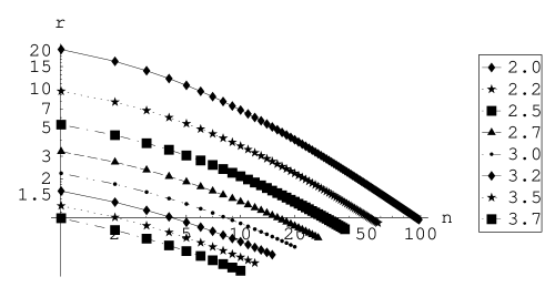
We numerically integrated the above equation to derive the ratio between the degree of a node and the expected degree of its richest neighbor. The ratio is plotted in Figure 2. For a range of exponents and node degrees, the expected degree of the richest neighbor is higher than the node itself. However, eventually (the precise point depends strongly on the power-law exponent), the probability of finding an even higher degree node in a neighborhood of a very high degree node starts falling.

What this means is that one can approximately follow the degree sequence across the entire graph for a sufficiently small graph or one with a power-law exponent close to 2 ($2.0<\tau<2.3$). At each step one chooses a node with degree higher than the current node, quickly finding the highest degree node. Once the highest degree node has been visited, it will be avoided, and a node of approximately second highest degree will be chosen. Effectively, after a short initial climb, one goes down the degree sequence. This is the most efficient way to do this kind of sequential search, visiting highest degree nodes in sequence.

3 Simulation

We used simulations of a random social network with a power-law link distribution of $\tau=2.1$ to validate our analytical results. As in the analysis above, a simple cutoff at $m\sim N^{1/\tau}$ was imposed. The expected number of nodes among N having exactly the cutoff degree is 1. No nodes of degree higher than the cutoff are added to the graph. In real world graphs one of course does observe nodes of degree higher than this imposed cutoff, so that our simulations become a worse case scenario. Once the graph is generated, the largest connected component (LCC) is extracted, that is the largest subset of nodes such that any node can be reached from any other node. For $2<\tau<3.48$ a giant connected component exists [13], and all our measurements are performed on the LCC. We observe that the LCC contains the majority of the nodes of the original graph and most of the links as well. The link distribution of the LCC is nearly identical to that of the original graph with a slightly smaller number of 1 and 2 degree nodes.

Next we apply our message passing algorithm to the network. Two nodes, the source and the target, are selected at random. At each time step the node which has the message passes it on to one of its neighbors. The process ends when the message is passed on to a neighbor of the target. Since each node knows the identity of all of its neighbors, it can pass the message directly to the target if the target happens to be one of it’s neighbors. The process is analogous to performing a random walk on a graph, where each node is ’visited’ as it receives the message.

There are several variants of the algorithm, depending on the strategy and the amount of local information available.

1. The node can pass the message on to one of its neighbors at random, or it can avoid passing it on to a node which has already seen the message.

2. If the node knows how many neighbors it has, it can choose to pass the message onto the neighbor with the most neighbors.

3. The node may know only its neighbors, or it may know who its neighbors’ neighbors are. In the latter case it would pass the message onto a neighbor of the target.

In order to avoid passing the message to a node that has already seen the message, the message itself must be signed by the nodes as they receive the message. Further, if a node has passed the message, and finds that all of its neighbors are already on the list, it puts a special mark next to its name, which means that it is unable to pass the message onto any new node. This is equivalent to marking nodes as follows:

white

Node hasn’t been visited.

gray

Node has been visited, but all its neighbors have not.

black

Node and all its neighbors have been visited already.

Here we compare two strategies. The first performs a random walk, where only retracing the last step is disallowed. In the message passing scenario, this means that if Bob just received a message from Jane, he wouldn’t return the message to Jane if he could pass it to someone else. The second strategy is a self avoiding walk which prefers high degree nodes to low degree ones. In each case both the first and second degree neighbors are scanned at each step.

Figure 3: Scaling of the average node to node search time in a random power-law graph with exponent 2.1, for random and high degree seeking strategies.

Figure 4: Scaling of the time required to cover one half the graph for random and high degree seeking strategies.

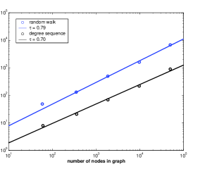
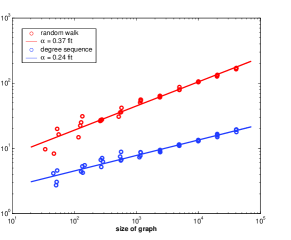
Figure 4 shows the scaling of the average search time with the size of the graph for the two strategies. The scaling (exponent 0.79 for the random walk and 0.70 for the high degree strategy) is not as favorable as in the analytic results derived above ($0.14$ for the random walk and 0.1 for the high degree strategy when $\tau=2.1$) .

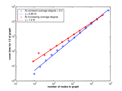
Consider, on the other hand, the number of steps it takes to cover half the graph. For this measure we observe a scaling which is much closer to the ideal. As shown in Figure 4, the cover time scales as $N^{0.37}$ for the random walk strategy vs. $N^{0.15}$ from Equation 19. Similarly, the high degree strategy cover time scales as $N^{0.24}$ vs. $N^{0.1}$ in Equation 24.

The difference in the value of the scaling exponents of the cover time and average search time implies that a majority of nodes can be found very efficiently, but others demand high search costs. Figures 6 and 6 show just that. A large portion of the 10,000 node graph is covered within the first few steps, but some nodes take as many steps or more to find as there are nodes total. Take for example the high degree seeking strategy. About 50% of the nodes are scanned within the first 10 steps (meaning that it would take about $10+2=12$ hops to reach 50% of the graph). However, the skewness of the search time distribution bring the average number of steps needed to 217.

Figure 5: Distribution of number of nodes seen as a function of the number of steps taken for random walk and high degree strategies for a 10,000 node graph.

Figure 6: Cumulative distribution of number of nodes seen as a function of the number of steps taken for random walk and high degree strategies for a 10,000 node graph.

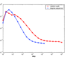
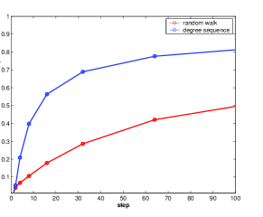
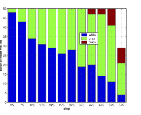
Figure 8 illuminates why some nodes take such a long time to find. It shows the color of nodes visited in a random walk on a $N=1000$ node power-law graph with exponent 2.1 and an abrupt cutoff at $N^{1/2.1}$. The number of nodes of each color encountered in 50 step segments is recorded in the bar for that time period.

The brief initial period where many white nodes are visited is followed by a long period dominated by gray and black nodes. The random walk starts retracing its steps, only occasionally encountering a new node it hasn’t seen. Close to the end of the walk, even the gray nodes have been exhausted as the random walk repeatedly visits back nodes before it finds the final few nodes.

Figure 7: Bar graph of the color of the nodes visited in a random walk on a 1,000 node power-law graph with exponent 2.1.

Figure 8: Bar graph of the color of nodes visited in strategic search of a random 1,000 node power-law graph with exponent 2.1.

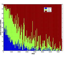
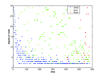
A self-avoiding high-degree seeking random walk is an improvement over the random walk described above, but still cannot avoid retracing its steps. Figure 8 shows the corresponding bar chart in 50 step increments. Comparing figures 8 and 8 we observe that the self-avoiding strategy is somewhat effective, with the total number of steps needed to cover the graph about 13 times smaller, and the fraction of visits to gray and black nodes significantly reduced. Figure 9 shows the degree in addition to the color of the node visited at every step. It demonstrates that one is able to follow the degree sequence initially, going from high degree white nodes to low degree white nodes.

Figure 9: Color and degree of nodes visited in a strategic search of a random 1,000 node power-law graph with exponent 2.1.

Although the strategy of revisiting nodes modifies the scaling behavior, it is not the process of revisiting itself which necessarily changes the scaling. If nodes were uniformly linked, at every step the number of new nodes seen would be proportional to the number of unexplored nodes in the graph. The factor by which the search is slowed down through revisits would be independent of the size of the graph. Hence, revisiting alone does not account for the difference in scaling.

The reason why the simulated scaling exponents for these search algorithms do not follow the ideal is the same reason why power-law graphs are so well suited to search: the link distribution is extremely uneven. A large number of links point to only a small subset of high degree nodes. When a new node is visited, its links do not let us uniformly sample the graph, they preferentially lead to high degree nodes, which have likely been seen or visited in a previous step. This would not be true of a Poisson graph, where all the links are randomly distributed and hence all nodes have approximately the same degree. We will explore and contrast the search algoritm on a Poisson graph in the following section.

4 Comparison with Poisson Distributed Graphs

In a Poisson random graph with $N$ nodes and $z$ edges, the probability $p=z/N$ of an edge between any two nodes is the same for all nodes. The generating function $G_{0}(x)$ is given by [12]:

$$G_{0}(x)=e^{z(x-1)}$$ (29)

In this special case $G_{0}(x)=G_{1}(x)$, so that the distribution of outgoing edges of a node is the same whether one arrives at the vertex by following a link or picks the node at random. This makes analysis search in a Poisson random graph particularly simple. The expected number of new links encountered at each step is a constant $p$. So that the number of steps needed to cover a fraction $c$ of the graph is $s=cN/p$. If $p$ remains constant as the size of the graph increases, the cover time scales linearly with the size of the graph. This has been verified via simulation as shown in Figure 10.

In our simulations the probability $p$ grows slowly towards its asymptotic value as the size of the graph is increased because of the particular choice of cutoff at $m\sim N^{(1/\tau)}$ for the power-law link distribution. We generated Poisson graphs with the same number of nodes and links for comparison. Within this range of graph sizes, growth in the average number of links per node appears as $N^{0.6}$, making the average number of 2nd degree neighbors scale as $N^{0.15}$. This means that the scaling of the cover time scales as $N^{0.85}$, as shown in Figure 10. Note how well the simulation results match the analytical expression. This is because nodes can be approximately sampled in an even fashion by following links.

Figure 10: Scaling of cover time for 1/2 of the graph for a Poisson graph with A) a constant average degree/node, and B) the same average degree/node as a power-law graph with exponent 2.1.

Figure 11: Fraction of nodes revisited in a given time interval vs. fraction of nodes visited in the graph for a search in A) a Poisson graph, and B) a power-law graph.

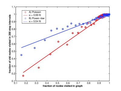
The reason why the cover time for the Poisson graph matches the analytical prediction and the power-law graph does not is illustrated in Figure 11. If links were approximately evenly distributed among the nodes, then if at one point in the search 50% of the graph has already been visited, one would expect to revisit previously seen nodes about 50% of the time. This is indeed the case for the Poisson graph. However, for the power-law graph, when 50% of the graph has been visited, nodes are revisited about 80% of the time, which implies that the same high degree nodes are being revisted before new low-degree ones. It is this bias which accounts for the discrepancy between the analytic scaling and the simulated results in the power-law case.

However, even the simulated $N^{0.35}$ scaling for a random, minimally self-avoiding strategy on the power-law graph out-performs the ideal $N^{0.85}$ scaling for the Poisson graph. It’s also important to note that the the high degree node seeking strategy has a much greater success in the power-law graph because it relies heavily on the fact that the number of links per node varies considerably from node to node. To illustrate this point, we executed the high degree seeking strategy on two graphs, Poisson and power-law, with the same number of nodes, and the same exponent $\tau=2$. In the Poisson graph, the variance in the number of links was much smaller, making the high degree node seeking strategy comparatively ineffective as shown in Figure 12.

Figure 12: Degrees of nodes visited in a single search for power-law and poisson graphs of 10,000 nodes.

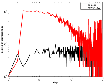
In the power-law graph we can start from a randomly chosen node. In this case the starting node has only one link, but two steps later we find ourselves at a node with the highest degree. From there, one approximately follows the degree sequence, that is, the node richest in links, followed by the second richest node, etc. The strategy has allowed us to scan the maximum number of nodes in the minimum number of steps. In comparison, the maximum degree node of the exponential graph is 11, and it is reached only on the 81st step. Even though the two graphs have a comparable number of nodes and edges, the exponential graph does not lend itself to quick search.

5 Gnutella

Gnutella is a peer-to-peer filesharing system which treats all client nodes as functionally equivalent and lacks a central server which can store file location information. This is advantageous because it presents no central point of failure. The obvious disadvantage is that the location of files is unknown. When a user wants to download a file, she sends a query to all the nodes within a neighborhood of size $ttl$, the time to live assigned to the query. Every node passes on the query to all of its neighbors and decrements the $ttl$ by one. In this way, all nodes within a given radius of the requesting node will be queried for the file, and those who have matching files will send back positive answers.

This broadcast method will find the target file quickly, given that it is located within a radius of $ttl$. However, broadcasting is extremely costly in terms of bandwidth. Every node must process queries of all the nodes within a given $ttl$ radius. In essence, if one wants to query a constant fraction of the network, say 50%, as the network grows, each node and network edge will be handling query traffic which is proportional to the total number of nodes in the network.

Such a search strategy does not scale well. As query traffic increases linearly with the size of Gnutella graph, nodes become overloaded as was shown in a recent study by Clip2 [3]. 56k modems are unable to handle more than 20 queries a second, a threshold easily exceeded by a network of about 1,000 nodes. With the 56k nodes failing, the network becomes fragmented, allowing users to query only small section of the network.

Figure 13: Log-log plot of the link distribution in the Gnutella network. The fitted exponent $\tau=2.07$.

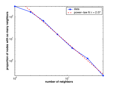
The search algorithms described in the previous sections may help ameliorate this problem. Instead of broadcasting a query to a large fraction of the network, a query is only passed onto one node at each step. The search algorithms are likely to be effective because the Gnutella network has a power-law connectivity distribution as shown in Figure 13.

Typically, a Gnutella client wishing to join the network must find the IP address of an initial node to connect to. Currently, ad hoc lists of ”good” Gnutella clients exist [3]. It is reasonable to suppose that this ad hoc method of growth would bias new nodes to connect preferentially to nodes which are already fairly well-connected, since these nodes are more likely to be ”well-known”. Based on models of graph growth [2, 8] where the ”rich get richer”, the power-law connectivity of ad hoc peer-to-peer networks may be a fairly general topological feature.

By passing the query to every single node in the network, the Gnutella algorithm fails to take advantage of its connectivity distribution. To implement our algorithm the Gnutella clients must be modified to keep lists of the files stored by their first and second degree neighbors have. This information must be passed at least once when a new node joins the network, and it may be necessary to periodically update the information depending on the typical lifetime of nodes in the network. Instead of passing the query to every node, queries are only passed along to the highest degree nodes. The IP numbers of the nodes already queried are appended to the query, and they are avoided.

The modified algorithm places an additional cost on every node, that of keeping track of the filenames of its neighbors’ files. Since network connections saturated by query traffic are a major weakness in Gnutella, and since computational and storage resources are likely to remain much less expensive than bandwidth, such a tradeoff is readily made. However, now instead of every node having to handle every query, queries are routed only through high connectivity nodes. Since nodes can select the number of connections that they allow, high degree nodes are presumably high bandwidth nodes that can handle the query traffic. The network has in effect created local directories valid within a two link radius. It is resilient to attack because of the lack of a central server. As for power-law networks in general [1], the network is more resilient than random graphs to random node failure, but less resilient to attacks on the high degree nodes.

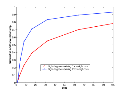
Figure 14 shows the success of the high degree seeking algorithm on the Gnutella network. We simulated the search algorithm on a crawl by Clip2 of the actual Gnutella network of approximately 700 nodes. Assuming that every file is stored on only one node, 50% of the files can be found in 8 steps or less. Furthermore, if the file one is seeking is present on multiple nodes, the search will be even faster.

To summarize, the power-law nature of the Gnutella graph means that these search algorithms can be effective. As the number of nodes increases, the (already small) number of nodes that will need to be queried increases sub-linearly. As long as the high degree nodes are able to carry the traffic, the Gnutella network’s performance and scalability may improve by using these search strategies.

Figure 14: Cumulative number of nodes found at each step in the Gnutella network.

6 Conclusion

In this paper we have shown that local search strategies in power-law graphs have search costs which scale sub-linearly with the size of the graph, a fact that makes them very appealing when dealing with large networks. The most favorable scaling was obtained by using strategies which preferentially utilize the high connectivity nodes in these power-law networks. We also established the utility of these strategies for searching on the Gnutella peer-to-peer network.

It may not be coincidental that several large networks are structured in a way that naturally facilitates search. Rather, we find it likely that these networks could have evolved to facilitate search and information distribution. Networks where locating and distributing information, without perfect global information, plays a vital role tend to be power-law with exponents favorable to local search.

For example, large social networks, such as the AT&T call graph and the collaboration graph of film actors, have exponents in the range ($\tau=2.1-2.3$) which according to our analysis makes them especially suitable for searching using our simple, local algorithms. Being able to reach remote nodes by following intermediate links allows communication systems and people to get to the resources they need and distribute information within these informal networks. At the social level, our analysis supports the hypothesis that highly connected individuals do a great deal to improve the effectiveness of social networks in terms of access to relevant resources [6].

Furthermore, it has been shown that the Internet backbone has a power-law distribution with exponent values between 2.15 and 2.2 [11], and web page hyperlinks have an exponent of 2.1 [2]. While in the Internet there are other strategies for finding nodes, such as routing tables and search engines, one observes that our proposed strategy is partially used in these systems as well. Packets are routed through highly connected nodes, and users searching for information on the Web turn to highly connected nodes, such as directories and search engines, which can bring them to their desired destinations.

On the other hand, a system such as the power grid of the western United States, which does not serve as a message passing network, has an exponent $\tau\sim 4$ [2]. It would be fairly difficult to pass messages in such a network without knowing the target’s location.

Acknowledgement

We would like to thank Clip2 for the use of their Gnutella crawl data.

References

- [1] R. Albert, H. Jeong, and A.-L. Barabasi. Error and attack tolerance of complex networks. Nature, 406:378, 2000.
- [2] Albert-Laszlo Barabasi and Reka Albert. Emergence of scaling in random networks. Science, 286:509, 1999.
- [3] Clip2. Gnutella: To the bandwidth barrier and beyond. http://www.clip2.com/gnutella.html, 2000.
- [4] Clip2. Reflector. http://dss.clip2.com/reflector.html, 2000.
- [5] P. Erdös and A. Rényi. On the evolution of random graphs. Publ. Math. Inst. Hung. Acad. Sci., 5:17–61, 1960.
- [6] Malcolm Gladwell. The Tipping Point: How Little Things Can Make a Big Difference. Little Brown & Company, New York, NY, 2000.
- [7] Theodore Hong. In Andy Oram, editor, Peer-to-Peer: Harnessing the Benefits of a Disruptive Technology, chapter 14, pages 203–241. O’Reilley, 2001.
- [8] B.A. Huberman and L.A. Adamic. Growth dynamics of the world wide web. Nature, 401:131, 1999.
- [9] H. Jeong, B. Tombor, R. Albert, Z. N. Oltvai, and A.-L. Barabasi. The large-scale organization of metabolic networks. Nature, 407(6804):651–654, 2000.
- [10] Jon M. Kleinberg. Navigation in a small world. Nature, 406:845, 2000.
- [11] P. Faloutsos M. Faloutsos and C. Faloutsos. On power-law relationships of the internet topology. In SIGCOMM, pages 251–262, 1999.
- [12] Mark Newman. Random graphs with arbitrary degree distribution and their applications. Phys. Rev. E, submitted.
- [13] Fan Chung William Aiello and Linyuan Lu. A random graph model for massive graphs. In STOC ’00, Proceedings of the thirty-second annual acm symposium on Theory of computing, pages 171–180, 2000.