CONSTRUCTION OF AN ALGORITHM IN PARALLEL FOR THE FAST FOURIER TRANSFORM

Abstract

It has been designed, built and executed a code for the Fast Fourier Transform (FFT), compiled and executed in a cluster of $2^{n}$ computers under the operating system MacOS and using the routines MacMPI. As practical application, the code has been used to obtain the transformed from an astronomic imagen, to execute a filter on its and with a transformed inverse to recover the image with the variates given by the filter. The computers arrangement are installed in the Observatorio Astronómico National in Colombia under the nameOAN Cluster, and in this has been executed several applications.

Key words. Fast Fourier Transform, message passing interface (MPI), paralelling processing.

1 Introduction

In the last few years, the implementation of low-cost computer nets for processing in parallel has been growing. Most of the designated implementations denominate “Clusters” have been developed in work stations under environments of Unix; however today exits Clusters that include the processing G3-G4 of Motorola-IBM-Apple, in computers Apple Macintosh running under MacOS,[2] and also with Pentium III under Linux or Windows.[1]

TheOAN Cluster is a project that born in December of 1998 motivated by the reached developments for Decyk and his team [3], by the hardware (Macs/G3) recently incorporate to the Observatorio Astronómico Nacional (OAN) and by the developments in software carried out within the investigation lines: Theoretical Astrophysics, Galactic Astronomy and Numerical Methods of the OAN. With the support of Absoft Corporation [4] was incorporated an excellent software compiler (Fortran 77/90 and C, C ++); that together with the routines MacMPI developed by Decyk in [5] completed the development structure of the OAN Cluster.

The first codes were centered in the knowledge of the own commands of the MPI, to evolve in the data distribution and operations with matrix. Several applications have been developed, one of them the denominated “prime numbers under the rule of Stanislav Ulam” the one which is found available in the Web address of the OAN [6] and an algorithm in parallel for the Fast Fourier Transform.

2 Fast Fourier Transform

Let $f:\mathbb{R}\to\mathbb{C}$ a continuously function, where $R$ represents the set of real numbers and $C$ the complex numbers. The Fourier Transform of $f$ is given by

$$H(\nu)=\int_{-\infty}^{\infty}f(t)e^{-2\pi i\nu t}dt,$$ (1)

where $i$ is the imaginary unity and $\nu$ the frecuency [7].

In most of practical situations, the function $f$ is given in discrete form as a finite values collection $f(x_{0}),f(x_{1}),\dots,f(x_{N-1})$ with $N\in\mathbb{N}$, where $\mathbb{N}$ is the set of natural numbers and {$x_{0},x_{1},\dots,x_{N-1}$} is one partition on an real interval $[a,b]$ and $x_{k}=a+\frac{b-a}{N}k$, for $0\leq k\leq N-1$. In problems that imply numerical calculation, instead the equation (1) we use the sum partial

$$H(k)={1\over N}\sum_{j=0}^{N-1}f(x_{j})e^{-2\pi ikj/N},$$ (2)

designated Discrete Fourier Transform (DFT) of $f$ over the interval $[a,b]$. If $f$ is a function defined on the interval $[0,2\pi]$ of real value with period $2\pi$, the values $H(k)$, by $k=0,\dots,N-1,$ can be interpreted as the coefficients $c_{k}$

$$c_{k}=\frac{1}{N}\sum_{j=0}^{N-1}f(x_{j})e^{-i\frac{2\pi k}{N}j},\qquad\hbox{$0\leq k\leq N-1$ }$$ (3)

of a exponential polynomial

$$p(x)=\sum_{k=0}^{N-1}c_{k}e^{ikx},$$ (4)

where $x\in\mathbb{R}$, $c_{k}\in\mathbb{C},$ y $k=0,1,\dots,N-1,$ which interpole $f$ in the values $f(x_{0}),f(x_{1}),\ldots,f(x_{N-1}).$

The Discrete Fourier Transform of $f$ over the partition $\{x_{0},x_{1},\dots,x_{N-1}\},$ is defined as the operator

$$DFT:\mathbb{C}^{N}\longrightarrow\mathbb{C}^{N}$$

such that

$[c_{0},c_{1},\ldots,c_{N-1}]^{T}=DFT\Big{(}[f(x_{0}),f(x_{1}),\ldots,f(x_{N-1})]^{T}\Big{)}$

The algorithm that evaluates DFT is denominated Fast Fourier Transform, and reduces the calculation significantly. For directly calculations is necesary to use $N^{2}$ multiplications, while FFT only needes $NLog_{2}N$ products. A comparison for greater values of $N$ is shown in Table 2.

The next tree show how is running the interpolation. In the first level (indicated by the superscript of the polynomials) are related two data in each branch that comes of the zero level and produce a polynomial with two coefficients $P_{k}^{(1)},$ for $0\leq k\leq 3$. In the second level, again the points gene- rated are interpolated and produces new factors and polynomials $P_{k}^{(2)},$ with $0\leq k\leq 1$; Finally we obtain the output vector, where $P_{0}^{(3)}$ is the polynomial that we requires .

$P_{0}^{(3)}$
                                           $\nearrow$              $\nwarrow$
                          $P_{0}^{(2)}$                                            $P_{1}^{(2)}$
                          $\nearrow\nwarrow$                                            $\nearrow\nwarrow$
             $P_{0}^{(1)}$                  $P_{2}^{(1)}$                       $P_{1}^{(1)}$                  $P_{3}^{(1)}$
             $\nearrow\nwarrow$                  $\nearrow\nwarrow$                       $\nearrow\nwarrow$                   $\nearrow\nwarrow$
     $P_{0}^{(0)}$          $P_{4}^{(0)}$      $P_{2}^{(0)}$       $P_{6}^{(0)}$          $P_{1}^{(0)}$           $P_{5}^{(0)}$     $P_{3}^{(0)}$          $P_{7}^{(0)}$

The parallel code works $2^{l}$ processors, $l\geq 0$. For a better comprehension let us consider an example: let $C=[C(0),\ldots,C(7)]$ eight data and four processors.

The basic variables that are used, are presented in Table 1. Then, for this example we have: $nproc=4$, $N=8$, $m=3$, $m1=1$.

Table 1: Basic variables

Variable	Description
$nproc$	Number of processors.
$idproc$	Label correspondent to each processor.
	We have $0\leq idproc<nproc$, with the processor $0$ equal to MASTER.
$N$	number of data.
$C$	Vector with the data.
$Z$	Vector with factors $e^{-\frac{2\pi i}{N}j}$, $0\leq j\leq N-1$.
$m$	Number of tree’s levels calculated for $\Big{[}\frac{Log(N)}{Log(2)}\Big{]}$.
$n$	Number of level in the process, $0\leq n<m$.
$m1$	Number of level until work all processors, $m-\Big{[}\frac{Log(nproc)}{Log(2)}\Big{]}$.
$nproc\_sup$	Number of processors in some levels.

Each processor works with its respective branch:

$idproc=0$           $idproc=2$              $idproc=1$          $idproc=3$
                $P_{0}^{(1)}$                  $P_{2}^{(1)}$                        $P_{1}^{(1)}$                    $P_{3}^{(1)}$
               $\nearrow\nwarrow$                  $\nearrow\nwarrow$                       $\nearrow\nwarrow$                   $\nearrow\nwarrow$
      $P_{0}^{(0)}$          $P_{4}^{(0)}$      $P_{2}^{(0)}$       $P_{6}^{(0)}$          $P_{1}^{(0)}$           $P_{5}^{(0)}$     $P_{3}^{(0)}$          $P_{7}^{(0)}$
      $C(0)$         $C(4)$     $C(2)$      $C(6)$        $C(1)$        $C(5)$     $C(3)$        $C(7)$

In this step, the processor identified with the label $idproc$ generates the coefficients’ vector: $P^{(n)}_{idproc}$ for $0\leq idproc<nproc=4;$ ($n=1$). The processing of the information continues until $n=m1=1$. In this point $idproc=2$ transmits its vector to $idproc=0,$ and $idproc=3$ transfers its vector to $idproc=1$. Before of the transference, each processor stores the information in a matrix with two columns where the real part is stored in the first column and the imaginary part in the second column. This is necessary because the commando to send don’t recognize complex numbers in language C.

In this moment $idproc=2$ and $idproc=3$ don’t work. Moreover, $nproc\_sup=\frac{nproc}{2}=2,$ so, in the level $n=2$ the number of processors is reduced to the half. From now on, where we avanced of level, the middle of processors out of the game and the variable $nproc\_sup$ descend to the middle.

The processors that receive the information unpack in $C$.

$idproc=0$                                   $idproc=1$
                            $P_{0}^{(2)}$                                            $P_{1}^{(2)}$
                    $C(0)$     $C(2)$                                 $C(4)$     $C(6)$
                    $C(1)$     $C(3)$                                 $C(5)$     $C(7)$
                          $\nearrow\nwarrow$                                            $\nearrow\nwarrow$
                   $P_{0}^{(1)}$       $P_{2}^{(1)}$                               $P_{1}^{(1)}$         $P_{3}^{(1)}$

In the level $n=2$, $idproc$ bring about the vector of coefficients $P^{(n)}_{idproc}$ for $0\leq idproc<nproc\_sup=2$. That which is stated previously, is repeated while $nproc\_sup\geq 1$, that is to say, while exist one processor. The MASTER receive the communication of $idproc=1$ and effects the last calculation to bring out $P^{(n)}_{idproc}$ ($idproc=0$ and $n=m=3$), in this instant $nproc\_sup=\frac{1}{2}$ and the process finish.

3 THE INVERSE TRANSFORM

We affirm that the exponential polinomyal (4) estimates the Inverse Discrete Fourier Transform (IDFT), definied as the operator

$$IDFT:\mathbb{C}^{N}\longrightarrow\mathbb{C}^{N}$$

such that

$[f(x_{0}),f(x_{1}),\ldots,f(x_{N-1})]^{T}=IDFT\Big{(}[c_{0},c_{1},\ldots,c_{N-1}]^{T}\Big{)}$

We use the FFT to calculate the IFFT. We define $x_{k}=\frac{2\pi k}{N}$ for
$0\leq k\leq N-1$, and evaluate $p$ in $2\pi-x_{k}=2\pi-\frac{2\pi k}{N}$

$$p(2\pi-x_{k})=\sum_{j=0}^{N-1}c_{j}e^{ij(2\pi-x_{k})}=\sum_{j=0}^{N-1}c_{j}e^{ij2\pi}c_{j}e^{-ijx_{k}}=\sum_{j=0}^{N-1}c_{j}e^{-ijx_{k}}=N\Big{(}\frac{1}{N}\sum_{j=0}^{N-1}c_{j}e^{-ijx_{k}}\Big{)}$$ (5)

In this way obtain the IFFT estimating the FFT multiplied for $N$ and

$$p(2\pi-x_{k})=p(2\pi-\frac{2\pi k}{N})=p\Big{(}2\pi\frac{N-k}{N}\Big{)},$$

so the inverse transform is in contrary order.

4 COMPLEXITY COMPUTATIONAL OF FFT IN PARALLEL

If the number of data is $N=2^{m}$ ($m\geq 1$) and the number of processors is $2^{l}$ ($l\geq 0$), the order of complex multiplications effected until the level $m1$, correspond to the multiplications made for each processor with its respective branch. The number of multiplications carried out until the level $n$ is $n2^{m}$ for $0\leq n\leq m.$ Particulary, if $n=m1$ we have $O(m1(2^{m}))$. Then dividing for the number of processors, the complexity descend to

$$\frac{m1(2^{m})}{2^{l}}=(m1)2^{m-l}=m1(2^{m1})$$

for $n=m1$.

Finally we adds the number of multiplications effected in the levels $n$, for $m1<n\leq m.$ In each level we have $2^{m}$ products. Considering that for each level $n$, $m1<n\leq m,$ the number of processors is reduced to the middle, obtain

$$\sum_{i=1}^{l}2^{m1+i}$$

from $m1+1$ until $n=m$.
Summarizing,

$$O\Big{(}(m-l)2^{m-l}+\sum_{i=1}^{l}2^{m-l+i}\Big{)}.$$ (6)

Calculating the ratio between sequential FFT and parallel FFT, we have

$$\frac{NLog_{2}N}{(m-l)2^{m-l}+\sum_{i=1}^{l}2^{m-l+i}} = \frac{m2^{m}}{(m-l)2^{m-l}+\sum_{i=1}^{l}2^{m-l+i}}$$

$$= \frac{m}{(m-l)2^{-l}+\sum_{i=1}^{l}2^{-l+i}}$$

This indicate that the algorithm in parallel is $\frac{m}{(m-l)2^{-l}+\sum_{i=1}^{l}2^{-l+i}}$ faster than the sequential algorithm.

Table 2: Comparative arithmetic products

$N$	$N^{2}$	$NLog_{2}N$	Pfp	RSP FFT
512	262144	4608	1664	2.77
2048	4194304	22528	7680	2.93
8192	67108864	106496	34816	3.06
32768	1073741824	491520	155648	3.16

Pfp: Paralell with four processors.
RSP FFT: Ratio between sequential and paralell FFT.

5 THE TWO-DIMENSIONAL DISCRETE TRANSFORM 2D-DFT

For two variables the sample is in $xy$-plane where the sample is uniformly distribuited in the parallel straight-lines to the $x$-axis (rows) and the parallel straight-lines $y$-axis (columns). We define $\mathcal{M}_{N\times M}(\mathbb{C})$ the matrix of size $N\times M$ which contain complex numbers. Let $f(x,y):\mathbb{R}^{2}\longrightarrow\mathbb{C}$ be a two-dimensional function, its 2D-DFT is definied as the operator

$$2D-DFT:\mathcal{M}_{N\times M}(\mathbb{C})\longrightarrow\mathcal{M}_{N\times M}(\mathbb{C})$$

$\Big{(}f(x,y)\Big{)}_{N\times M}\mapsto\Big{(}F(u,v)\Big{)}_{N\times M}$
where

$$F(u,v)=\frac{1}{N}\sum_{x=0}^{N-1}\sum_{y=0}^{M-1}f(x,y)e^{-i2\pi(\frac{ux}{N}+\frac{vy}{M})}$$ (7)

for $u=0,1,\ldots,N-1,v=0,1,\ldots,M-1.$
And we establish the 2D-IDFT (Inverse Discrete Fourier Transform two-dimensional) as

$$2D-IDFT:\mathcal{M}_{N\times M}(\mathbb{C})\longrightarrow\mathcal{M}_{N\times M}(\mathbb{C})$$

$\Big{(}F(u,v)\Big{)}_{N\times M}\mapsto\Big{(}f(x,y)\Big{)}_{N\times M}$
where

$$f(x,y)=\frac{1}{M}\sum_{u=0}^{N-1}\sum_{v=0}^{M-1}F(u,v)e^{i2\pi(\frac{ux}{N}+\frac{vy}{M})}$$ (8)

for $x=0,1,\ldots,N-1,y=0,1,\ldots,M-1.$

The equation (7) we express as

$$F(u,v)=\frac{1}{N}\sum_{x=0}^{N-1}\sum_{y=0}^{M-1}f(x,y)e^{-i2\pi\frac{ux}{N}}e^{-i2\pi\frac{vy}{M}}=\frac{1}{N}\sum_{x=0}^{N-1}F(x,v)e^{-i2\pi\frac{ux}{N}}$$ (9)

where $F(x,v)=M\Big{(}\frac{1}{M}\sum_{y=0}^{M-1}f(x,y)e^{-i2\pi\frac{vy}{M}}\Big{)}$. In this way, we may frequent use of the DFT on rows and on columns.

The implementation of the algorithm for the 2D-FFT (Fast Fourier Transform two-dimensional) is,

FFT on rows $\longrightarrow$ Multiplication for $M$ $\longrightarrow$ FFT on columns. [9]

6 APPLICATION

A application has been diriged to the image processing. We can represent a image as a function

$f:\mathbb{R}^{2}\longrightarrow\mathbb{Z}$

$(x,y)\mapsto z=f(x,y)$

where $\mathbb{Z}$ is the set of integer numbers, $(x,y)$ is the coordinate image’s point with brightness $f(x,y)$. A digital image, it’s a image which $x,y,f(x,y)\in\mathbb{Z}^{+}\cup\{0\}$. Thus, a image is a two-dimensional array $(P_{x,y})_{N\times M}$ of pixels (picture elements).

The algorithm pads with zeros on rows and on columns to complete the next power of two.

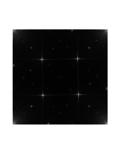
The Fourier Transform we can represent trought of its spectrum

$$\sqrt{Re[C(x,y)]^{2}+Im[C(x,y)]^{2}}$$ (10)

where $Re[C(x,y)]$ is the real part and $Im[C(x,y)]$ is the imaginary part of the Transform’s element $(x,y)$.

A images’ filter is a operator $H:\mathbb{Z}^{2}\longrightarrow\mathbb{R}$ which permits to change the brightness in the digital image. For the Convolution Theorem we can use a filter and to multiply it with the real and imaginary part image’s Fourier Transform. A filter can be designed either to eliminate or to create noise in a image. We use the filter:

$$F\left({x,y}\right)=\left\{{\matrix{{0\ }\cr{1\ }\cr}\matrix{{si\ \sqrt{\left({x-c_{1}}\right)^{2}+\left({y-c_{2}}\right)^{2}}\leq b}\cr{en\ caso\ contrario\ \ \ \ \ \ \ \ \ \ \ \ \ \ \ \ }\cr}}\right.$$ (11)

where $(c_{1},c_{2})$ is the image’s center and $b>0$, [9].

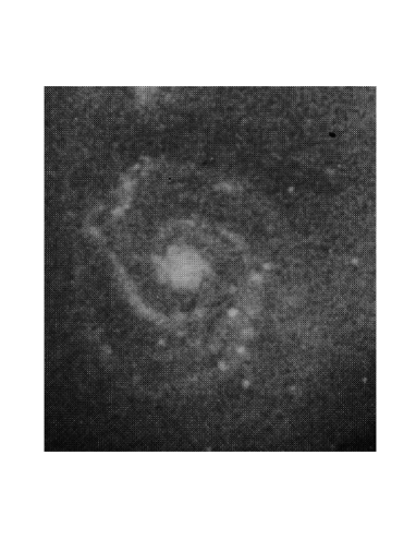
Finally, we calculate the 2D-IFFT to this product and obtain the image filtered. In the next step, we can see the smoothing effect derived using the filter over the spiral galaxy NGC5194 (Whirpool Galaxy). This picture has a size of 460$\times$506 pixels, and was taken of [10]; in our work we use a filter parameter of $b=340$.

Figure 1: Original galactic picture

Figure 2: Fourier spectrum

Figure 3: Transformed picture

7 SUMMARY AND CONCLUSIONS

1. Arithmetical expression for number of multiplications in the parallel FFT was obtained in the equation (6) and calculated the ratio between sequential and paralell FFT products (with four processors) for four values of $N$, listed in Table 2.

2. We write until the proper functioning the algorithm 2D-FFTp.c. using the MPI’s routines and tools of MacOS system.

3. We find that the efficiency increase when the communications has the minimum rate of transference executing the code in the cluster.

4. We build the filter of the equation (11) and had been applied to the galaxy NGC5194 obtaining a new image (figure 3) which the high frequency’s components had been eliminated.

We acknowledge an anonymous referee for this helpful coments. We thank Viktor K. Decyk in UCLA for his useful recommendatios and permanent   assistance. This work has been supported by DIB of the Universidad Nacional de Colombia through Proyect DIB-803577.