On the predictability of Rainfall in Kerala
An application of ABF Neural Network

Abstract

Rainfall in Kerala State, the southern part of Indian Peninsula in particular is caused by the two monsoons and the two cyclones every year. In general, climate and rainfall are highly nonlinear phenomena in nature giving rise to what is known as the ‘butterfly effect’. We however attempt to train an ABF neural network on the time series rainfall data and show for the first time that in spite of the fluctuations resulting from the nonlinearity in the system, the trends in the rainfall pattern in this corner of the globe have remained unaffected over the past 87 years from 1893 to 1980. We also successfully filter out the chaotic part of the system and illustrate that its effects are marginal over long term predictions.

1 Introduction

Although technology has taken us a long way towards better living standards, we still have a significant dependence on nature. Rain is one of nature’s greatest gifts and in third world countries like India, the entire agriculture depends upon rain. It is thus a major concern to identify any trends for rainfall to deviate from its periodicity, which would disrupt the economy of the country. This fear has been aggravated due to the threat by the global warming and green house effect. The present study has a soothing effect since it concludes that in spite of short term fluctuations, the general pattern of rainfall in Kerala has not undergone major deviations from its pattern in the past.

The geographical configuration of India with the three oceans, namely Indian Ocean, Bay of Bengal and the Arabian sea bordering the peninsula gives her a climate system with two monsoon seasons and two cyclones inter-spersed with hot and cold weather seasons. The parameters that are required to predict the rainfall are enormously complex and subtle so that the uncertainty in a prediction using all these parameters is enormous even for a short period. The period over which a prediction may be made is generally termed the event horizon and in best results, this is not more than a week’s time. Thus it is generally said that the fluttering wings of a butterfly at one corner of the globe may cause it to produce a tornado at another place geographically far away. This phenomenon is known as the butterfly effect.

The objective of this study is to find out how well the periodicity in these patterns may be understood using a neural network so that long term predictions can be made. This would help one to anticipate with some degree of confidence the general pattern of rainfall for the coming years. To evaluate the performance of the network, we train it on the rainfall data corresponding to a certain period in the past and cross validate the prediction made by the network over some other period. A difference diagram is plotted to estimate the extent of deviation between the predicted and actual rainfall. However, in some cases, the cyclone may be either delayed or rushed along due to some hidden perturbations on the system, for example an increase in solar activity. (See figure 2.) These effects would appear as spikes in the difference diagram. The information from the difference diagram is insufficient to identify the exact source of such spike formation. It might have resulted from slight perturbations from unknown sources or could be due to an inaccurate modeling of the system using the neural network. We thus use a standard procedure in statistical mechanics that can quantitatively estimate the fluctuations[1]. This is to estimate the difference in the Fourier Power Spectra (FPS) of the predicted and actual sequences. In the FPS, the power corresponding to each frequency interval, referred to as the spectral density gives a quantitative estimate of the deviations of the model from reality. Rapid variations would contribute to high frequency terms and slowly varying quantities would correspond to low frequency terms in the power spectra.

The degree of information that may be extracted from the FPS is of great significance. If the model agrees with reality, the difference of the power spectra ( hereafter referred to as the residual FPS ) should enclose minimum power in the entire frequency range. An exact model would produce no difference and thus no residual FPS pattern. If there are some prominent frequency components in the residue, that could indicate two possibilities; either the network has failed to comprehend the periodicity, or that there is a new trend in the real world which did not exist in the past. One can test whether the same pattern exists in the residual FPS produced on the training set and confirm whether it is a new trend or is the drawback of the model.

A random fluctuation would be indicated in the residual FPS by amplitudes at all frequency values as in the case of ‘white’ noise spectra. Here again, how much power is enclosed within the FPS gives a quantitative estimate of the perturbations. A low amplitude fluctuation can happen due to so many reasons. But its effect on the overall predictability of the system would be minimal. If however, the residual FPS encloses a substantial power from the actual rainfall spectrum, the fluctuations could be catastrophic.

In this study, the results indicate that the perturbations produced by the environment on the rainfall pattern of Kerala state in India is minimal and that there is no evidence to envisage a significant deviation from the rainfall patterns prevailing here.

The general outline of the paper is as follows. In section 2 we present a brief outline of the Adaptive Basis Function Neural Network (ABFNN), a variant of the popular back-propagation algorithm. In section 3, the experimental set up is explained followed by the results and concluding remarks in section 4.

2 Adaptive Basis Function Neural Networks

It was shown in [2] that a variant of the back-propagation algorithm (backprop) known as the Adaptive Basis Function Neural Network performs better than the standard backprop networks in complex problems. The ABFNN works on the principle that the neural network always attempts to map the target space in terms of its basis functions or node functions. In standard backprop networks, this function is a fixed sigmoid function that can map between zero and plus one or between minus one and plus one the input applied to it from minus infinity to plus infinity. It has many attractive properties that make the backprop an efficient tool in a wide variety of applications. However serious studies conducted on the backprop algorithm have shown that in spite of its widespread acceptance, it systematically outperforms other classification procedures only when the targeted space has a sigmoidal shape [3]. This implies that one should choose a basis function such that the network may represent the target space as a nested sum of products of the input parameters in terms of the basis function. The ABFNN thus starts with the standard sigmoid basis function and alters its nonlinearity by an algorithm similar to the weight update algorithm used in backprop.

Instead of the standard sigmoid function, ABFNN opts for a variable sigmoid function defined as

$$O_{f}=\frac{a+tanh(x)}{1+a}$$ (1)

Here $a$ is a control parameter that is initially set to unity and is modified along with the connection weights along the negative gradient of the error function. It is claimed in [2] that such a modification could improve the speed and accuracy with which the network could approximate the target space.

The error function is computed as:

$$E=\sum_{k}\frac{\left(O_{k}-O_{k}^{*}\right)^{2}}{2}$$ (2)

with $O_{k}$ representing the network output and $O_{k}^{*}$ representing the target output value.

With the introduction of the control parameter, the learning algorithm may be summarized by the following update rules. It is assumed that each node, $k$, has an independent node function represented by $a_{k}$. For the output layer nodes, the updating is done by means of the equation:

$$\qquad\Delta a_{k}=-\beta\left(O_{k}-O_{k}^{*}\right)\frac{1-O_{k}}{1+a_{k}}$$ (3)

where $\beta$ is a constant which is identical to the learning parameter in the weight update procedure used by backprop.

For the first hidden layer nodes, the updating is done in accordance with the equation:

$$\Delta{\textit{a}}_{k-1}=-\sum_{i}w_{ij}\beta\left(O_{k}-O_{k}^{*}\right)\left(1-O_{k}\right)\left[\left(1+{\textit{a}}_{k}\right)+O_{k}\left(1+{\textit{a}}_{k}\right)\right]\frac{\partial O_{k}}{\partial O_{k-1}}$$ (4)

Here $w_{ij}$ is the connection weight for the propagation of the output from node $i$ to node $j$ in the subsequent layer in the network.

The introduction of the control parameter results in a slight modification to the weight update rule ($\Delta w_{ij}$) in the computation of the second partial derivative term $\frac{\partial O_{j}}{\partial I_{j}}$ in:

$$\Delta w_{ij}=-\beta\frac{dE}{dw_{ij}}=-\beta\frac{\partial E}{\partial O_{j}}\frac{\partial O_{j}}{\partial I_{j}}\frac{\partial I_{j}}{\partial w_{ij}}$$ (5)

as:

$$\frac{\partial O_{j}}{\partial I_{j}}=\left[\left(1-a_{j}\right)+\left(1+a_{j}\right)O_{j}\right]\left(1-O_{j}\right)$$ (6)

The algorithm does not impose any limiting values for the parameter $a$ and it is assumed that care is taken to avoid division by zero.

3 Experimental setup

In pace with the global interest in climatology, there has been a rapid updating of resources in India also to access and process climatological database. There are various data acquisition centers in the country that record daily rainfall along with other measures such as sea surface pressure, temperature etc. that are of interest to climatological processing. These centers are also associated to the World Meteorological Organization (WMO). The database used for this study was provided by the Department of Atmospheric Sciences of Cochin University of Science and Technology, a leading partner in the nation wide climatological study centers.

The database consists of the rainfall data from Trivandrum in Kerala, situated at latitude-longitude pairs ($8^{o}29^{\prime}$ N - $76^{o}57^{\prime}$ E). Although the rainfall data from 1842 were recorded, there were many missing values in between that we had to restrict to periods for which a continuous time series was available. This was obtained for the period from 1893 to 1980.

For training our network, the Trivandrum database from 1893 to 1933 was used. Since rainfall has an yearly periodicity, we started with a network having 12 input nodes. It was observed that the network accuracy would systematically improve as we increased the number of input nodes from 12 to 48 covering the data corresponding to 4 years. Any increase in input nodes resulted in poorer representations. Further experimentation showed that it was not necessary to include information corresponding to the whole year, but a 3 month information centered over the predicted month of the fifth year in each of the 4 previous years would give good generalization properties. We thus finalized our network with 12 input nodes each for the 3 months input data over 4 years, 7 hidden nodes and one output node. Thus, based on the information from the four previous years, the network would predict the amount of rain to be expected in each month of the fifth year.

The training was carried out until the root mean-square error stabilized to around 0.085 over the training data(40 years from 1893-1933). The ABFNN converged to this value in around 1000 iterations starting from random weight values and took less than 10 minutes on a 300MHz PC using Celeron processor and Linux operating system.

After training, the data corresponding to the entire 87 years of rainfall in Trivandrum city was presented to the network. The output from the network was compared with the actual data in the time series. In addition to visual comparison, the spectral analysis was also done on the test dataset to obtain a quantitative appreciation of the performance of the network.

4 Results and Discussion

In figure 1 we show the difference pattern produced by the network over the entire 87 year period on the Trivandrum database. The training period is also shown. It may be noted that the deviations of the predicted signal from the actual in the entire dataset falls within the same magnitude range. The root mean square error on the independent test dataset was found to be around 0.09. The two positive spikes visible in the plot corresponding to the two instances where the rainfall was delayed with reference to the month for which it was predicted are shown in figure 2.

The cause for the negative spike in figure 1 is also seen in figure 2 as due to the deviation of the time series from the predicted upward trend. Factors such as the El-Nino southern oscillations (ENSO) resulting from the pressure oscillations between the tropical Indian Ocean and the tropical Pacific Ocean and their quasi periodic oscillations are observed to be the major cause of these deviations in the rainfall patterns[4].

To obtain a quantitative appreciation of the learning algorithm, we resort to the spectroscopic analysis of the predicted and actual time series. The average power per sample distributed in the two sequence is shown in figure 3. It is seen that the two spectra compare very well. To identify the differences, the deviation of the FPS (residual FPS) of the predicted sequence from the actual in the months following the training period was plotted . For comparison, The deviation of the FPS of the actual rainfall patterns in this period from that of the training period was also plotted. The resulting graphs are shown in figure 4. In attempting to predict the evolution of the system in the months following the training period, it is to be noted that the deviation of the spectra of the predicted sequence for this period is less than that of the Fourier spectra corresponding to the training period. This is because the network attempts to learn the behavior of a system where as Fourier analysis means only a transformation from time domain to frequency domain. Also Fourier analysis assumes the system to be stationary, which is not true in the case of rainfall phenomena. Comparing the FPS of the network output corresponding to the training period showed the existence of residual frequency components at 1 Hz and 3 Hz, as seen in the residual FPS of figure 4. They represent the error bars or the inherent uncertainty to be expected in the prediction of the quantum of rainfall due to those oscillations. The information for learning such fluctuations is not in the time series data. Future studies shall include other climatic parameters such as temperature, sea surface pressure, solar activity etc. in conjunction with the time series information in an attempt to reduce the error bars in the prediction. The rest of the spectra is spread over the entire frequency range producing random fluctuations in the rainfall phenomena.

Thus it is to be concluded that other than minor fluctuations, the power factor in the residual FPS is insignificant to expect any major deviations in the rainfall pattern prevailing in the country.

It is also to be noted that the ABF neural network is a better tool than the popular Fourier analysis methods for predicting long term rainfall behavior. The learning ability of the network can give a concise picture of the actual system where as the Fourier spectra is only a transformation from time domain to frequency domain, assuming that the time domain sequence is stationary. It thus fails to represent the dynamics of the system which is inherent in most natural phenomena and rainfall in particular.

Acknowledgment

The authors wish to express their sincere thanks to Professor K. Mohankumar of the Department of Atmospheric Sciences of the Cochin University of Science and Technology for providing us with the rainfall database and for useful discussions. The first author would like to thank Dr. Moncy V John of the Department of Physics, Kozhencherri St. Thomas college for long hours of discussions.

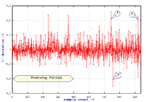
Figure 1: The deviation of the predicted sequence from the actual time series data is shown. It may be noted that the deviations in the training period and the rest of the series are comparable in magnitude. The larger spikes are mainly due to the delay in the actual commencement of the monsoon or cyclone. Label 1 indicates an example where the monsoon extended into the following month giving more rainfall than anticipated. Label 2 in the figure represent an example where the monsoon was actually delayed by one month than was anticipated thus producing two spikes, one negative and the other positive. Label 3 corresponds to a negative spike caused by the change in trend from the predicted increase in rain in the following year.

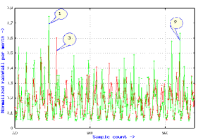
Figure 2: An overlap of the predicted and the actual time series data in the region corresponding to the spikes in figure 1 is shown. The labels indicate the reason for the spikes seen in figure 1.

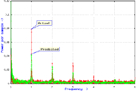
Figure 3: The Fourier power spectra corresponding to the actual and the predicted rainfall for the entire 87 years. The sampling frequency does not have much significance here since the sample values represent the total rain received in each month. It was taken to be twelve to associate itself with the 12 months of the year. Since FPS is symmetric over half the sampling frequency, we show here only values from 0 to 6.

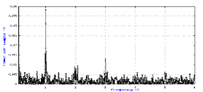
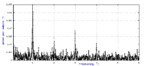
Figure 4: The residual FPS corresponding to the predicted and actual rainfall in the years following the training period is shown on top. The spectral difference from a Fourier analysis perspective (the difference of the FPS in the training period and the period corresponding to the top figure) is presented in the bottom figure. Note that the spectral differences are minimum in the top figure. This is to say that the deviations observed in the actual spectra in the bottom figure followed from the trend associated with the training period.

References

- [1] E. S. R. Gopal, Statistical Mechanics and Properties of Matter Theory and Applications, Ellis Horwood, 1974.
- [2] N. S. Philip and K. B. Joseph, Adaptive Basis Function for Artificial Neural Networks, (in press) Neurocomputing Journal, also available at http://www.geocities.com/sajithphilip/research.htm
- [3] M. A. Kraaijveld Small sample behaviour of multi-layer feed forward network classifiers: Theoretical and Practical Aspects (Delft University Press, 1993).
- [4] A. Chowdhury and S. V Mhasawade, Variations in meteorological floods during summer monsoon over India, Mausam, 42, 2, 167-170, 1991.