A Price Dynamics in Bandwidth Markets for Point-to-point Connections

Abstract

We simulate a network of $N$ routers and $M$ network users making concurrent point-to-point connections by buying and selling router capacity from each other. The resources need to be acquired in complete sets, but there is only one spot market for each router. In order to describe the internal dynamics of the market, we model the observed prices by $N$-dimensional Itô-processes. Modeling using stochastic processes is novel in this context of describing interactions between end-users in a system with shared resources, and allows a standard set of mathematical tools to be applied. The derived models can also be used to price contingent claims on network capacity and thus to price complex network services such as quality of service levels, multicast, etc.

1 Introduction

To be able to provide guaranteed quality of service, QoS, in a network, a user needs to be able to reserve capacity, or ’bandwidth’, in congested routers. The reservation scheme should be efficient in the sense that one reservation should not unnecessarily block other reservations, and it should not require extensive negotiation. One scheme that fits these requirements is to trade router capacity in spot markets. The assumption is that someone reserves capacity for a connection by buying the capacity in the routers along the cheapest path between the source and destination node. When the capacity is no longer needed, it is sold to someone else. Increased demand increases price, so alternative paths, if they exist, may become competitive, and the users will tend to move their bandwidth usage away from congested routers.

We ultimately want to be able to price contingent claims on resources, formalized as options or futures. The working hypothesis is that adding a suitable set of such claims will improve the efficiency of the resource allocation, as prices will better reflect all available information. Indeed, the purpose of contingent claims on future value, such as options, futures, or more generally, derivative securities, is to construct a market for trading the expected future value. For the problem studied here, this means trading in expected future demand and supply. One way to price derivatives is to use statistical modeling of the price dynamics, since under suitable assumptions, which we will cover in a forthcoming separate contribution, derivative prices are functions of current market prices and the statistical model[Black73][Avellaneda99]. This paper addresses the necessary preliminary issue of how to estimate parameters in two stochastic models from observed market prices, and also presents measures of the efficiency of the market resource allocation scheme. These questions are also of independent interest, as the efficiency is to be used to compare different market system with each other, and with other allocation schemes.

Using artificial markets for resource allocation in distributed systems dates back to the mid 80ies, ranging over markets for storage capacity [Kurose89], CPU time [Ferguson88] [Waldspurger92], and network capacity [Kurose85] [Sairamesh95]. The emphasis has been on evaluating the efficiency of the resource allocation, rather than understanding the resulting price dynamics. More recent work stresses the agent aspect, i.e. that the trading parties are locally optimizing entities [Faratin00]. Combinatorial markets, i.e. trading of bundles of distinct resources is yet a relatively new area. Somewhat related is the area of combinatorial auctions [Rassenti82] [Rothkopf98] [Sandholm99]. The use of derivatives for network admission control has been used in [Lazar98].

Previous bandwidth market models usually only include a primary market, in which end-users can buy and sell capacity only from the router owner. In the presented model end-users trade amongst each other, i.e. the capacity is traded on secondary markets.

This paper is organized as follows: in section 2 we present the model, of which a central ingredient is a detailed mechanism of price formation, with very low overhead in user-user communication. In section 3 we model mathematically the resulting price processes. The main tools used are stochastic differential equations (Itô-processes), their associated Fokker-Planck equations, and the stationary distribution of those. In section 4 we sum up an discuss our results.

2 Method

2.1 Market model

Figure 1: The network with 10 routers.

We simulate a network consisting of $N$ inter-connected routers and $M$ network users concurrently making reservations of router capacity for point-to-point connections. There is one spot market per router, in which users trade router capacity.

We use Farmer’s non-equilibrium market dynamics [Farmer00] as a prescription of how prices change due to trading (see also sec. 4). Farmer’s model is based on the assumption of a market maker that guarantees liquidity at all times, and that buying causes prices to increase, while selling causes prices to decrease. Farmer assumes that the price dynamics is such that it is impossible to move the market by performing a sequence of trades, where the net traded volume is zero, and that the relative price changes are independent of the current value of the price. From these assumptions, Farmer derives a formula that the price per unit in a transaction of $\omega$ units is $\tilde{S}(S,\omega)=Se^{\omega/\lambda}$, where $S$ is the unit price in the previous trade, and $\lambda$ the market depth or liquidity, i.e. the rate at which the price is changed by trading. For a derivation, see Appendix A. This model is useful since we do not have to simulate details of the order-book in each market. Instead, we can calculate the price change caused by trading directly from the last price and the size of the trade.

2.2 Simulation setup

At each time interval, $m$ new demands are generated. A demand is a 7-tuple,

$$d\equiv<id,uid,src,dst,cap,dur,max>$$

The user identities are chosen independently, so one user may receive zero or one or several new demands. If the current time is $t,$ demand $id$ specifies that the user $uid$ demands $cap$ units in each node on a path from $src$ to $dst$, starting at time $t$ and ending at time $t+dur$ if it costs less than $max$ to obtain the resources. If there are several paths, a choice will be made, see below. During the simulation a user reserves capacity in a router by buying that capacity, and sells excess capacity that is no longer in need.

User $i$ owns $r_{i,j}$ units of $j$. Initially, none of the simulated users are assigned any resources or money, i.e. $r_{i,j}=0,\,cash_{i}=0$ for all $i$ and $j$, nor do they have any resource demand, $\omega_{i,j}=0$. When a user manages to satisfy a demand, its capital is increased by the amount $max$, and when resources are bought and sold, the capital is decreased and increased, respectively, by the cost of the resource. The simulation is run in $L$ time steps from time $0$ to $T$ with time increments $\Delta t$. At each time step where the current time is $t$:

• Generate $m$ new demands. A demand is specified by a unique demand number $id$, a user $uid$ randomly drawn from the set of $M$ users, a source node $src$ and a destination node $dst$, both randomly drawn from the set of $N$ nodes, and the required capacity per node $cap$, which is randomly drawn as the ceiling of $e^{K\xi}$ where $\xi$ is a uniform random variable between 0 and 1. If some demand is more important than others, a user is willing to pay more for that resource. In this simulation, $max$ is a linear function of the required capacity, i.e. the maximum total cost $max=C_{unit}\,cap$, where $C_{unit}$ is a simulation parameter. The duration (number of time steps) $dur$ is randomly drawn integer between $1$ and $D$.

• Calculate $\omega_{i,j}$, the net change of resource $j$ of user $i=uid$ in the following way:

  • For each new demand $d$, user $i$ looks at the last known transaction prices $S_{j}(t)$ and decides to buy $cap$ resources along the least cost path. Since the user will not know the actual cost of a buying and later selling resources along a path, its decision on whether to buy resources or not, is determined by a parameter $C_{max}$. The user decides to buy the resources if and only if the estimated total cost to buy the resources is less than $C_{max}max$. The resulting demand $cap$ is then added to the $\omega_{i,j}$ for all the resources $j$ on the least cost path, and the amount $max$ is added to $cash_{i}$.

  • For each satisfied demand $d$ terminating at $t$, decide to sell the resources that were allocated (if any) to the demand, i.e. subtract the resulting supply of liberated capacity on the least cost path if the demand was satisfied and router capacity was bought.

• All the demands on capacity in single routers (i.e. $\omega_{i,j}$) are effectuated one by one in random order, and for each trade prices are updated to $S_{j}e^{\omega_{i,j}/\lambda_{j}}$. The $cash_{i}$ is decreased by $\omega_{i,j}S_{j}$ and the owned amount of resource is increased by $\omega_{i,j}$. According to the price formation formula, the trades are made at prices which depend on the actual order. The prices payed by the users are thus not the same as those used for determining the least cost path. The next known price is the one that pertains after all the trades, and is independent of the order.

• When all trading is done for this time-step, log the last transaction prices, $\hat{S}(t)$, the number of satisfied demands, and repeat.

2.3 Simulation Parameters

The simulation was run for $L=1000$ time-steps ($\Delta t=0.01)$ using the network in (fig. 1). There were $10$ routers and 10 users, so $N=10$ and $M=10$. The liquidity in all Farmer markets was chosen to be $\lambda_{i}=10$. The maximal cost per route users were willing to accept was determined by $C_{unit}=100$ and $C_{max}=1$ for all users. Initial prices were set to $\hat{S}_{i}(0)=10$ in all markets. Every time step, $m=10$ new demands were generated. The duration $dur$ was uniformly distributed between $1$ and $10$, i.e. $D=10$. The call duration sets the time scale in the simulation, as we will see below. The required amount of capacity was determined by $K=2$ (see above).

3 Results

price
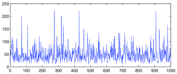
	time

Figure 2: Plot of the unit price of capacity in router 1 from time 0.01 to 10. $\Delta t$=0.01.

3.1 Statistical modeling of the price process

Inhomogeneous drift, additive noise, constant coefficients

The price as shown in (fig. 2) does not appear to be drifting freely. Instead it appears to return towards the same area. Assuming the price process is an Ornstein-Uhlenbeck process, the dynamics for the price of router $i$ would be

$$dS_{i}(t)=\alpha_{i}\big{(}\mu_{i}-S_{i}(t)\big{)}dt+\sigma_{i}dW_{i}(t)$$ (1)

where $W_{i}(t)$ is a Wiener process and the correlation between two processes $i$ and $j$ is $Corr[dW_{j}(t),dW_{j}(t)]=\rho_{i,j}$. Recall that a Wiener process has independent normal distributed increments with mean $0$ and variance $t-s$, i.e. $W_{i}(t)-W(s_{i})\sim N[0,\sqrt{t-s}]$ where $t>s$. For improved readability, we omit the indices in $S_{i}(t)$, etc., when they are irrelevant for the understanding.

In (eq. 1) the drift term (the $dt$ term) detracts when $S$ is bigger than $\mu$, and adds when $S$ is less than $\mu$. The amount of the increase is determined by $\alpha$. The diffusion (the $dW$ term) is independent of $S$.

When the simulation has run for sufficiently long time, the price $S_{i}(t)$ becomes independent of the starting state of the system, and reaches a stationary distribution $P(t)$ of $S(t)$. Using the Fokker-Planck equation (see Appendix A) gives

$$P(s)=C_{0}e^{-\frac{1}{2}\big{(}\frac{s-\mu}{\sigma/\sqrt{2\alpha}}\big{)}^{2}}$$ (2)

where $C_{0}=(\pi\sigma^{2}/\alpha)^{-\frac{1}{2}}$, which is the density function for a normal distribution $N[\mu,\frac{\sigma}{\sqrt{2\alpha}}]$. We note first that the normal distribution is non-zero in all of $(-\infty,\infty)$, meaning that $S(t)$ can take on negative values, something that is not possible in a market with Farmer’s dynamics. Second, the normal distribution has many good properties, such as that a weighted sum of normal distributed variables is also normal distributed. If prices are far from zero, this dynamics may therefore be a convenient approximation to the true distribution. Third, the stationary distribution only depends on the ratio $\frac{\sigma^{2}}{\alpha}$ and can therefore not distinguish between separate variations in $\sigma^{2}$ and $\alpha$, which has to be done by other means.

The observations $\hat{S}(i)$, $i\in[1,...,L]$ of the process $S$ in its stationary state are regularly spaced with distance $\Delta t$. Since $E[S]=\mu,$ we estimate $\mu$ with

$$\hat{\mu}=\hat{E}[S]=\frac{1}{L}\sum_{i=1}^{L}\hat{S}(i)$$

We estimate $\sigma$ after noting that $E[(dS)^{2}]=\sigma^{2}dt+O(dt\,dW)$. Therefore, for small $\Delta t$,

$$\hat{\sigma}^{2} = \frac{1}{\Delta t}\hat{E}[(dS)^{2}]$$

$$= \frac{1}{\Delta t}\frac{1}{L-1}\sum^{L-1}_{i=1}\Big{(}\hat{S}(i+1)-\hat{S}(i)\Big{)}^{2}$$

Since $Var[S]=\frac{\sigma^{2}}{2\alpha}$, the unbiased estimate is

$$\frac{\hat{\sigma}^{2}}{2\hat{\alpha}} = \frac{L}{L-1}\Big{(}\hat{E}[S^{2}]-\hat{E}[S]^{2}\Big{)}$$

so the estimate of $\alpha$ is

$$\hat{\alpha}=\frac{1}{2\Delta t}\frac{\sum^{L-1}_{i=1}\Big{(}\hat{S}(i+1)-\hat{S}(i)\Big{)}^{2}}{\Big{(}\sum^{L}_{i=1}\hat{S}(i)^{2}-\big{(}\sum^{L}_{i=1}\hat{S}(i)\big{)}^{2}\Big{)}}$$

density
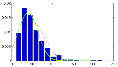
	price

Figure 3: Histogram over the observed prices, the estimated normal distributed density function $N[\mu,\sigma/\sqrt{2\alpha}]$ (the red dashed line), and a least square error fit to the 15 columns in the histogram (the green dotted line).

To verify that the observed estimate is indeed correct, we can plot the histogram of the observed data together with the estimated density function $P(s)$, see (fig 3). This estimation coincides with the maximum likelihood estimate of the variables. A least square fit to the values in the histogram gives a better-looking curve. However, this fit only gives $\mu$ and the ratio $\frac{\sigma^{2}}{\alpha}$, as noted above.

Having estimates of $\alpha$, $\mu$ and $\sigma$ we are able to estimate the correlation $\rho_{i,j}$ between the random sources for two price processes $S_{i}$ and $S_{j}$ by solving $dW_{i}$ and $dW_{j}$ in (eq. 1) and using the estimates

$$d\hat{W}_{i}(k)=\frac{\hat{S}_{i}(k+1)-\hat{S}_{i}(k)-\hat{\alpha}_{i}\big{(}\hat{\mu}_{i}-\hat{S}_{i}(k)\big{)}\Delta t}{\hat{\sigma}_{i}}$$

so that the estimate becomes

$$\hat{\rho}_{i,j} = \frac{\hat{\textrm{C}}\textrm{ov}[dW_{i},dW_{j}]}{{}^{\hat{\textrm{V}}\textrm{ar}[dW_{i}]\hat{\textrm{V}}\textrm{ar}[dW_{j}]}}$$

$$= \frac{\frac{1}{L-1}\sum^{L-1}_{k=1}d\hat{W}_{i}(k)d\hat{W}_{j}(k)}{(\Delta t)^{2}}$$

where we have used $E[dW]=0$ and $Var[dW]=dt$.

Inhomogeneous drift, multiplicative noise, constant coefficients

The dynamics in (sec. 3.1) can generate negative prices, something which is should not be possible in a well-functioning market. By asserting a mean-reverting dynamics with multiplicative noise we get a process that is strictly positive. Assume the dynamics for the price of router $i$ to be

$$dS_{i}(t)=\alpha_{i}\big{(}\mu_{i}-S_{i}(t)\big{)}dt+\sigma_{i}S_{i}(t)dW_{i}(t)$$ (3)

where $W_{i}(t)$ is a Wiener process and the correlation between two processes $i$ and $j$ is $Corr[dW_{j}(t),dW_{j}(t)]=\rho_{i,j}$. As before, we we omit the indices in $S_{i}(t)$, etc., for readability.

The stationary distribution $P(s)$ of $S$ is

$$P(s)=\frac{(\gamma\mu)^{\gamma}\mu}{\Gamma(\gamma)}e^{-\frac{\gamma\mu}{s}}\Big{(}\frac{1}{s}\Big{)}^{\gamma+2}$$ (4)

where $\gamma\equiv\frac{2\alpha}{\sigma^{2}}$, and $\Gamma(z)$ is the gamma function. In (eq. 4) $s$ takes only positive values, which is consistent, since the dynamics in (eq. 3) does not move an $s$ from positive to negative.

The first moment of this distribution, $E[S]$ is $\mu$ (see Appendix A). As for the Ornstein-Uhlenbeck process above, we estimate $\mu$ with

$$\hat{\mu}=\hat{E}[S]=\frac{1}{L}\sum_{i=1}^{L}\hat{S}(i)$$

We cannot easily estimate $\sigma$ from $E[(dS)^{2}]$ since $S$ is in the drift term, but note that the process $X(t)=\log(S(t))$ in (eq. 8) has additive noise. Therefore, we get for small $\Delta t$,

$$\hat{\sigma}^{2} = \frac{1}{\Delta t}\hat{E}[(dX)^{2}]$$

$$= \frac{1}{\Delta t}\frac{1}{L-1}\sum^{L-1}_{i=1}\Big{(}\log\frac{\hat{S}(i+1)}{\hat{S}(i)}\Big{)}^{2}$$

To estimate $\alpha$, we try two approaches. First we use the conditional expectation $E[S(t+\tau)|S(t)]$ for $S$ in the stationary state of the system. Taking the partial derivative w.r.t $\tau$ gives a first order ODE with the solution

$$E[S(t+\tau)|S(t)]=e^{-\alpha\tau}(S(t)-\mu)+\mu$$

showing that the expected value approaches $\mu$ exponentially with $\tau$ and $\alpha$ determines the speed of the return. Rearrange to keep $e^{-\alpha\tau}$ (which is independent of $S(t)$) on one side, take the logarithm and take the expected value of both sides. Let $\tau=k\Delta t$. We now have an estimate for $\alpha$,

$$exp(-\hat{\alpha}\,k\Delta t)=\frac{1}{L-k}\sum^{L-k}_{i=1}\frac{\hat{S}(i+k)-\hat{\mu}}{\hat{S}(i)-\hat{\mu}}$$

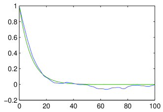
$e^{-\alpha\,k\Delta t}$		$\textrm{Cov}[S(t+k\Delta t),S(t)]$
	$k=\tau/\Delta t$		$k$

Figure 4: Left fig.: the estimate $\hat{y}=e^{-\alpha k\Delta t}$ derived from the conditional expectation of $S(t+\tau)$ for the first 20 time-steps in blue, and the plot of $y=e^{-\hat{\alpha}k\Delta t}$ in green. The estimate may be less than zero due to the noise from the simulation. Right fig.: the covariance between $S(t+k\Delta t)$ and $S(t)$. The auto-correlation deviates some from an exponential, possibly because the price dynamics has higher order than assumed. It would explain why the estimate in the left plot deviates from an exponential. Simulation time, $100\,000$ time steps, $\lambda_{i}=10,$ and $D=100$.

As we can see from the left hand side of the equation above, plotting the right hand side as a function of $k$ should result in a straight line if $\alpha$ is constant. However, as we can see in (fig. 4), the line is straight up to some $k$ that depends on the simulation parameters and error. The estimation is very sensitive to errors in $\hat{\mu}$, especially in the denominator if $\hat{S}$ is near $\hat{\mu}$, which results in a flattened out jagged line, since $e^{-\hat{\alpha}\,k\Delta t}$ is less than the simulation error for larger $k$. It eventually flattens out which means that $\alpha$ appears to decrease for larger $\tau$.

density
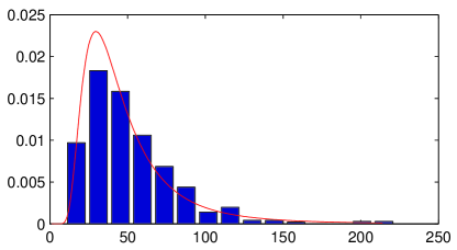
	price

Figure 5: Histogram over the observed prices and the estimated gamma distribution. $\mu$ and $\sigma$ are estimated using the moment method, and after that, $\alpha$ is estimated with a least square error fit.

Another way to estimate $\alpha$ is to estimate $\mu$ and $\sigma$ as above, and then fit the observed distribution to the distribution (eq. 4) using the least square method. See (fig. 5) for a plot of the model fit.

Having estimates of $\alpha$, $\mu$ and $\sigma$ we are able to estimate the correlation $\rho_{i,j}$ between the random sources for two price processes in the same way as above, by solving $dW_{i}$ and $dW_{j}$ in (eq. 3) and using the estimates

$$\Delta\hat{W}_{i}(k)=\frac{\hat{S}_{i}(k+1)-\hat{S}_{i}(k)-\hat{\alpha}_{i}\big{(}\hat{\mu}_{i}-\hat{S}_{i}(k)\big{)}\Delta t}{\hat{\sigma}_{i}\hat{S}_{i}(k)}$$

so that the estimate becomes

$$\hat{\rho}_{i,j}=\frac{\frac{1}{L-1}\sum^{L-1}_{k=1}d\hat{W}_{i}(k)d\hat{W}_{j}(k)}{(\Delta t)^{2}}$$

where again we have used $E[dW]=0$ and $Var[dW]=dt$.

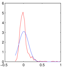
density		density
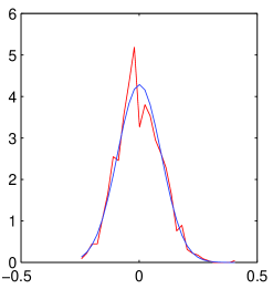
	$\Delta\hat{W}$		$\Delta\hat{W}$

Figure 6: The left figure shows the histogram (in red) over $\Delta\hat{W}$ in the simulation described in (sec.2.3) with $\lambda_{i}=10$, and a fitted density function for a normal distribution (in blue). The right figure shows the histogram of another simulation with the same parameters except for the market liquidity which is $\lambda_{i}=100$.

Plotting the histograms of $\Delta\hat{W}$ shows us if the model is good. If that is the case, the $\Delta\hat{W}$ should behave like samples of a Wiener process, i.e. be normal distributed. As can be seen in (fig. 6), the model (eq. 3) fits well if the market liquidity is high. However, if market liquidity is low then the assumed price model does not provide a good fit.

Price Correlations

The resource prices in a network of resources depend on the prices of other resources, since they are traded in groups. Using the parameter estimates of the price dynamics above, we get the correlation matrix in (tab. 1) for a simulation with high liquidity markets ($\lambda_{i}=100)$.

Router	1	2	3	4	5	6	7	8	9	10
1	1	0.33	-0.03	0.06	0.48	0.21	-0.05	0.08	-0.04	0.05
2		1	0.02	-0.12	0.06	-0.01	0.04	0.60	0.12	0.36
3			1	0.18	0.02	0.03	0.02	0.14	0.43	-0.03
4				1	0.38	0.40	0.20	-0.12	0.50	0.09
5					1	0.03	0.05	-0.09	0.11	-0.01
6						1	0.02	-0.11	0.09	0.46
7							1	0.15	0.45	-0.02
8								1	0.41	0.12
9									1	0.01
10										1

Table 1: Correlation coefficients for $\Delta\hat{W}$ for a simulation with $\lambda_{i}=100$, after 5000 time steps. Connected routers are in bold face.

We find that prices generally are positively correlated. Comparing with the network graph(fig. 1), one can see that prices of neighboring nodes often are strongly positively correlated with an average correlation coefficient of around 0.4, compared to 0.03 for nodes that are not connected. The most significant exception is nodes 3 and 7. Looking at the network graph it is clear that no least cost path can contain both 3 and 7, except for the path from 3 to 7.

3.2 Efficiency of the market based resource allocation

The efficiency of a market based resource allocation scheme depends on how well prices reflect the available information about resource demands. Two sources for bad performance is that price quotes are outdated, or that they do not reflect knowledge about the price behavior, e.g. periodic price fluctuations, or future prices. To measure efficiency, we can measure the resource utilization to compare which markets are able to capture most information.

Communication costs

The number of messages sent in the negotiation phase of this kind of system is negligible, since all users operate on old price quotes and place bids at market, i.e. accept the price whatever it may be. They do not update their price quotes for every bid. Therefore, less than $M$ messages per trade come in to a user (the potential quote update from each market). One message per trade (the bid) go out from each user to the markets that contain resources that the user have chosen. No messages need to be communicated between the end-users.

Successful connection ratio

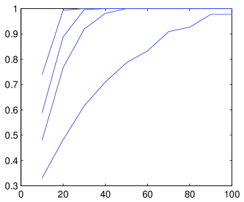
Successful connections		Avg. profit
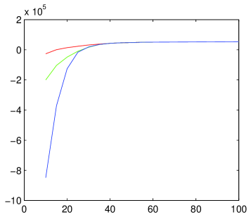
	$\lambda_{i}$		$\lambda_{i}$

Figure 7: To the left, average ratio of successful connections as a function of the market liquidity. The graphs from bottom to top have $C_{max}$ equal to 1, 4, 16 and 64. To the right, average net profit as a function of market liquidity. The graphs from bottom to top have $C_{max}$ equal to 64, 16, and 4, showing that a high $C_{max}$ causes losses on average in a low liquid market.

In the Farmer market model, the less liquid the markets are, the less valid are the price quotes. To the left in (fig. 7) the ratio of successful connections is plotted as a function of the market liquidity $\lambda_{i}$ for simulations with the parameters described in (sec. 2.3). The graphs corresponds to different values of the decision parameter $C_{max}$. Low liquidity causes large price fluctuations, making the prices higher than the limit $C_{max}max$ (see sec. 2.2) which inhibits many connections. Note that a connection is considered successful even if the net cost (after releasing the resources) is higher than $max$.

Net profit

To the right in (fig. 7) we plot the average profit as a function of the liquidity for a number of values of $C_{max}$. Large values of $C_{max}$ causes the users to buy resources when they are expensive. If the liquidity is high, the users sell resources at approximately the same price, but with low liquidity, prices will move significantly downwards when the resources are sold, causing a net loss to the user.

The particular way the $max$ cost for a connection is determined of course very much determines which of the different kinds of traffic that is promoted in the network. Different schemes could for instance promote short or long paths, high or low capacity connections, etc.

Average load

The average load, or reserved capacity in a router is with the Farmer dynamics a direct function of the market price, $\omega(t)=\lambda\log\frac{S(t)}{S(0)}$. If two simulations that allocate the same connections differ in load, the higher load depends on inefficient routing that does not choose efficient path. If the simulations differ in allocated connections, the comparison is less straight forward, and depends on the choice of metric above. We intend to return to a longer discussion on efficiency, in particular for load balancing, in a future contribution.

4 Discussion

In our simulation, Farmer’s market dynamics can be interpreted either as prescriptions of how a rational market maker should modify the market prices, or as a model of the aggregate behavior of market price changes during some period of time.

With the former interpretation, the Farmer dynamics can be used to implement a market maker program that brokers trading between end-users. The dynamics is derived from the assumption that it is impossible to change prices by ’trade in circles’. This assumption is a necessary condition for any market maker strategy, since otherwise anyone can exploit the market and gain an unlimited amount of money from the market maker.

The latter interpretation can be used when we want to simulate a part of a market with many concurrent trades. Since trading causes prices to change means that it is impossible to have updated price information at the time they place their bid. It is only possible to have completely updated price info if the trading is synchronous, something that severely reduces the number of bids a market can handle per time unit if communication delays are taken into account.

The market liquidity (or market depth) parameter $\lambda_{i}$ determines the speed at which prices change. When the dynamics interpreted as prescriptions for a market maker, it is up to the market maker to adjust $\lambda_{i}$ in order to reduce the risk of running out of resources. If we model an existing bandwidth market, $\lambda_{i}$ is an observable parameter which must be determined from the distribution of price jumps in relation to traded volume. The more resources in relation to the order size, the larger $\lambda_{i}$. A bandwidth market that is trading the capacity of a high capacity router can, everything else being equal, be expected to have a higher $\lambda_{i}$ than a similar market for a congested or inefficient router.

In the mean reverting processes investigated here, $\alpha$ determines the speed with which the process returns towards its statistical average $\mu$. The speed of return depends on the characteristic time length of the system, determined by the simulation parameter $D$, the call length. With a large $D$, the prices will be correlated with previous prices over a longer time period, which results in a small $\alpha$. With a small $D$, the price effect of previous calls will soon be forgotten, resulting in a high $\alpha$.

The traditional statistical models used for telephony have been found to inadequately model data network traffic. Data communication has been found to show a very bursty or fractal behavior as one communication event often generates a burst of more communication to other parts of the network. Data communication is generally short lived and often with strong latency bounds, due to the increasing use of computer networks for interactive communication. For short lived communication with low transfered amount, traditional switched best effort networks will probably continue to provide a very efficient solution for a long time. However, with increasing demand of streaming real-time data such as high quality video-telephony, video-on-demand, etc., it is necessary to be able to reserve capacity. The alternatives are large buffers, which has bad latency performance, or migrating data (intelligent replication), which can reduce load for one-to-many communication. Neither is suited for point-to-point communication service guarantees.

In the ’bandwidth market’ presented in this paper, end users buy the required resources themselves. The demand for updated price quotes results generates additional network traffic. In an extended model, we could allow risk neutral middle men to sell options on the resources. Since updated quotes will then only be required by the (few) middle men doing the actual trading, the additional traffic would be greatly reduced. We intend to return to these topics in future work.

Appendix A

Stationary Distribution

$S(t)$ is an Itô process with the dynamics $dS(t)=a(t,S(t))dt+b(t,S(t))dW(t)$, and $P(s,T;s_{0},t)$ is the contingent probability distribution of $S$ at time $T$ given $S(t)=s_{0}$. $P$ obeys the Fokker-Planck equation a.k.a the forward Kolmogorov equation,

$$-\partial_{T}P-\partial_{s}\Big{(}a(T,s)\,P\Big{)}+\partial_{ss}\big{(}\frac{b(T,s)^{2}}{2}P\big{)}=0$$ (5)

An important class of stochastic processes are those that are stationary. For those, if $T-t$ is sufficiently large, the contingent distribution $P$ no longer depends on $s_{0}$, and can be substituted with the stationary distribution $P(s)$, which does not depend on $s_{0}$, $t$ or $T$. Two ways in which a stochastic process can fail to be stationary is if the coefficients, e.g. $a$ and $b$, are explicitly time-dependent, or if there is no distribution $P(s)$. The latter happens for instance in ordinary random diffusion, in which the probability gradually spreads out without reaching a limit.

Assuming that a stationary distribution has been reached, the time derivative drops out of (eq. 5), and the equation can be integrated once to be

$$\partial_{s}P(s)-\frac{2a(s)-2b(s)\partial_{s}b(s)}{b(s)^{2}}P(s)=0$$ (6)

which is an ODE. One further integration of (eq. 6) gives

$$P(s)=C\,e^{\int_{0}^{s}\frac{2a(u)}{b(u)^{2}}du}\frac{1}{b(s)^{2}}$$ (7)

where $C$ is a normalization constant determined by $\int P(s)ds=1$.

The Additive Noise Process

Stationary density function, mean and variance

Assume the price dynamics

$$dS(t)=\alpha(\mu-S(t))dt+\sigma dW(t)$$

Then the conditional stationary probability distribution of $S$ is, using (eq. 7),

$$P(s) = C_{0}e^{-\frac{2\alpha}{\sigma^{2}}\int_{0}^{s}(\mu-u)du}$$

$$= C_{0}e^{-\frac{1}{2}\big{(}\frac{s-\mu}{\sigma/\sqrt{2\alpha}}\big{)}^{2}}$$

where $C_{0}=(\pi\sigma^{2}/\alpha)^{-\frac{1}{2}}$. $P(s)$ can be identified as the density function for a normal distribution with mean $\mu$ and variance $\sigma^{2}/2\alpha$.

The Multiplicative Noise Process

Stationary density function

Assume the price dynamics

$$dS(t)=\alpha(\mu-S(t))dt+\sigma SdW(t)$$

Using (eq. 7)

$$P(s) = C_{1}e^{\frac{2\alpha}{\sigma^{2}}\big{(}\int_{s_{0}}^{s}\frac{\mu}{u^{2}}du-\overbrace{\int_{s_{0}}^{s}\frac{1}{u}du}^{=\log s-\log s_{0}}\big{)}}\Big{(}\frac{1}{\sigma\,s}\Big{)}^{2}$$

$$= \frac{1}{C_{2}}e^{\frac{2\alpha}{\sigma^{2}}\big{(}-\frac{\mu}{s}\big{)}}\Big{(}\frac{1}{s}\Big{)}^{\frac{2\alpha}{\sigma^{2}}+2}$$

An alternative derivation is to let $X(t)=\log S(t)$. Itô’s lemma gives that

$$dX=\Big{(}\alpha\mu e^{-X}-(\alpha+\frac{\sigma^{2}}{2})\Big{)}dt+\sigma dW$$ (8)

Then the stationary probability distribution $Q(x)$ of $X$ is , using (eq. 7),

$$Q(x) = C_{0}e^{\int_{0}^{x}\big{(}-\frac{2\big{(}\alpha\mu e^{-X}-(\alpha+\frac{\sigma^{2}}{2})\big{)}}{\sigma^{2}}\big{)}du}\frac{1}{\sigma^{2}}$$

$$= C_{1}e^{-\gamma\mu e^{-x}+(\gamma+1)x}$$

where $C_{1}$ is a normalization constant, and $\gamma\equiv\frac{2\alpha}{\sigma^{2}}$ for readability. The stationary density function $P(s)$ for $S$ is found by recalling $X=\log(S)$ and

$$P(s)ds \equiv Q(\log(s))d(\log(s))$$

$$= \frac{1}{C_{2}}e^{-\gamma\mu\frac{1}{s}}\Big{(}\frac{1}{s}\Big{)}^{\gamma+1}\frac{1}{s}ds$$

The constant $C_{2}$ is determined by normalization and identifying the integral as a gamma function, $\Gamma(z+1)=\int^{\infty}_{0}t^{z}e^{-t}dt=z\Gamma(z)$. After the substitution $t=\gamma\mu\frac{1}{s}$ we get

$$C_{2} = \int^{0}_{\infty}e^{-t}\Big{(}\frac{1}{\gamma\mu}t\Big{)}^{\gamma+2}(-\gamma\mu\frac{1}{t^{2}})dt$$

$$= \Big{(}\frac{1}{\gamma\mu}\Big{)}^{\gamma+1}\int^{\infty}_{0}e^{-t}t^{\gamma}dt$$

$$= \Big{(}\frac{1}{\gamma\mu}\Big{)}^{\gamma}\frac{1}{\mu}\Gamma(\gamma)$$

Stationary mean

Use the same substitution, $t=\gamma\mu\frac{1}{s}$ to obtain

$$E[S] = \int^{\infty}_{0}sP(s)ds$$

$$= \int^{0}_{\infty}(\frac{1}{\gamma\mu}t)\frac{1}{C_{2}}e^{-t}\Big{(}\frac{1}{\gamma\mu}t\Big{)}^{\gamma+2}(-\gamma\mu\frac{1}{t^{2}})dt$$

$$= \frac{1}{C_{2}}\Big{(}\frac{1}{\gamma\mu}\Big{)}^{\gamma}\underbrace{\int^{\infty}_{0}e^{-t}t^{\gamma-1}dt}_{=\Gamma(\gamma)}$$

$$= \mu$$

Conditional expected value

Let $f(\tau|S(t))$ be the conditional expectation of $S(t+\tau)$ given $S(t)$.

$$f(\tau|S(t)) \equiv E[S(t+\tau)|S(t)]$$

$$= S(t)+E[\int_{t}^{t+\tau}dS(t^{\prime})|S(t)]$$

$$= S(t)+\alpha\mu\tau-\alpha\int_{t}^{t+\tau}E[S(t^{\prime})|S(t)]dt^{\prime}$$

Take the partial derivative with respect to $\tau$

$$\partial_{\tau}f(\tau|S(t)) = \alpha\mu-\alpha E[S(\tau)|S(t)]$$

$$= \alpha\mu-\alpha f(\tau|(S(t))$$

Multiplying with $e^{\alpha\tau}$ and collecting the terms gives

$$\partial_{\tau}\Big{(}e^{\alpha\tau}f(\tau|(S(t))\Big{)}=e^{\alpha\tau}\alpha\mu$$

Integrate both sides over $\tau$ from $0$ to $\tau$ and multiplication with $e^{-\alpha\tau}$ gives

$$f(\tau|S(t))=e^{-\alpha\tau}\big{(}S(t)-\mu\big{)}+\mu$$

where we have used that $f(0|S(t))=S(t)$. Therefore

$$e^{-\alpha\tau}=\frac{f(\tau|S(t))-\mu}{S(t)-\mu}$$

The left side does not depend on $S(t)$. Taking the expected value of both sides

$$e^{-\alpha\tau} = E[e^{-\alpha\tau}]$$

$$= E\Big{[}\frac{E[S(t+\tau)|S(t)]-\mu}{S(t)-\mu}\Big{]}$$

$$= \int_{0}^{\infty}\frac{E[S(t+\tau)|S(t)=x]-\mu}{x-\mu}P(x)dx$$

where $P$ is the stationary distribution of $S$, and we have substituted a time average with an ensemble average, which is true under suitable assumptions.

Estimation of parameter $\alpha$

We can estimate the integral from the observed data using the estimates

$$\hat{P}(x) \equiv \frac{1}{N}\sum_{t}\delta(x-\hat{S}(t))$$

$$\hat{E}[S(t+\tau)|S(t)=x] \equiv \frac{\sum_{t|\hat{S}(t)=x}\hat{S}(t+\tau)}{|\{x|\hat{S}(t)=x\}|}$$

where $\delta(x)$ is the Dirac delta function and $|A|$ is the cardinality of the set $A$. The estimation is

$$e^{-\hat{\alpha}\tau} \equiv \int_{0}^{\infty}\hat{P}(x)\frac{\hat{E}[S(t+\tau)|S(t)=x]-\hat{\mu}}{x-\hat{\mu}}dx$$

$$= \int_{0}^{\infty}\Big{(}\frac{1}{N}\sum_{t}\delta(x-\hat{S}(t))\Big{)}\hat{E}[\frac{S(t+\tau)-\hat{\mu}}{x-\hat{\mu}}|S(t)=x]dx$$

$$= \sum_{x|\hat{S}(t)=x}\frac{1}{N}|\{x|\hat{S}(t)=x\}|\frac{\sum_{t|\hat{S}(t)=x}\Big{(}\frac{S(t+\tau)-\hat{\mu}}{x-\hat{\mu}}\Big{)}}{|\{x|\hat{S}(t)=x\}|}$$

$$= \frac{1}{N}\sum_{t}\frac{\hat{S}(t+\tau)-\hat{\mu}}{\hat{S}(t)-\hat{\mu}}$$

so we can estimate $\alpha$ with

$$\hat{\alpha}(\tau)\equiv-\frac{1}{\tau}\log\Big{(}\frac{1}{N}\sum_{t}\frac{\hat{S}(t+\tau)-\hat{\mu}}{\hat{S}(t)-\hat{\mu}}\Big{)}$$

which should be a constant function.

Farmer’s market dynamics

Let $S$ be the current price, $\omega$ the net demand and $\tilde{S}$ the price at which the demand can be met. We seek a functional relationship of the type $\tilde{S}\equiv\tilde{S}(S,\omega)$, where $\tilde{S}$ depends continuously on $S$ and $\omega$. Assume the price to be positive and bounded, $\tilde{S}$ to be an increasing function of $\omega$, and that prices are only changed through trading, $\tilde{S}(S,0)=S$. Assume furthermore that one cannot make money by trading in circles

$$\tilde{S}(\tilde{S}(\tilde{S}(S,\omega_{1}),\omega_{2}),-(\omega_{1}+\omega_{2}))=S$$ (9)

and the relative price change is independent of the absolute price,

$$\frac{\tilde{S}(S,\omega)}{S}=\phi(\omega)$$ (10)

Because of (9) we see that $\tilde{S}(\tilde{S}(S,\omega),-\omega)=S$, so the inverse is $\tilde{S}^{-1}(S,\omega)=\tilde{S}(S,-\omega)$, where $\tilde{S}^{-1}$ is the inverse function of $\tilde{S}$. Applying $\tilde{S}^{-1}(\cdot,-(\omega_{1}+\omega_{2}))$ on (9) to see that

$$\tilde{S}(\tilde{S}(S,\omega_{1}),\omega_{2})=\tilde{S}(S,\omega_{1}+\omega_{2})$$ (11)

(10) together with (11) implies that $\phi(\omega_{1})\phi(\omega_{2})=\phi(\omega_{1}+\omega_{2})$ which implies $\phi(x)=e^{x/\lambda}$ for some constant $\lambda$. Therefore

$$\tilde{S}(S,\omega)=S\,e^{\omega/\lambda}$$ (12)

References

- [Avellaneda99] Marco Avellaneda and Peter Laurence, Quantitative Modeling of Derivative Securities: From Theory to Practice, CRC Press, 1999.
- [Black73] Fischer Black and Myron Scholes, The Pricing of Options and Corporate Liabilities, Journal of Political Economy, (81:3), pp. 637-654, 1973.
- [Faratin00] P. Faratin, N. R. Jennings, P. Buckle and C. Sierra. Automated Negotiation for Provisioning Virtual Private Networks using FIPA-Compliant Agents, Proc. of the 5th Int. Conf. on Practical Application of Intelligent Agents and Multi-Agent Systems (PAAM-2000), Manchester, UK. 2000.
- [Farmer00] J. Doyne Farmer, Market force, ecology, and Evolution, submitted to Journal of Economic Behavior and Organization, Feb. 2000.
- [Ferguson88] Donald Ferguson, Yechiam Yemini, and Christos Nikolaou, Microeconomic Algorithms for Load Balancing in Distributed Computer Systems, Proc. of the 8th Int. Conf. on Distributed Computer System, 1988.
- [Kurose85] James F. Kurose, Mischa Schwartz, and Yechiam Yemini, A Microeconomic Approach to Optimization of Channel Access Policies in Multi-Access Networks, Proc. of 5th Int. Conf. on Distributed Computer Systems, 1985.
- [Kurose89] James F. Kurose, and Rahul Simha, A Microeconomic Approach to Optimal Resource Allocation in Distributed Computer Systems, IEEE Trans. on Computers, (38) no. 5, May 1989.
- [Lazar98] Aurel A. Lazar, and Nemo Semret, Spot and Derivative Markets for Admission Control and Pricing in Connection-Oriented Networks, CU/CTR/TR 501-98-35, Columbia University, New York, 1998.
- [Rassenti82] S. J. Rassenti, V. L. Smith, and R. L. Buffin, A Combinatorial Auction Mechanism for Airport Time Slot Allocation, The Bell Journal of Economics, (13) pp. 402-417,1982.
- [Rothkopf98] Michael G, Rothkopf, Aleksandar Pekeč, and Ronald M. Harstad, Computationally Manageable Combinational Auctions, Management Science, (44) no. 8, Aug. 1998.
- [Sairamesh95] Jakka Sairamesh, Donald F. Ferguson, and Yechiam Yemini, An Approach to Pricing, Optimal Allocation and Quality of Service Provisioning In High-Speed Packet Networks, IEEE INFOCOM, 1995.
- [Sandholm99] Tuomas Sandholm, An Algorithm for Optimal Winner Determination in Combinatorial Auctions, Proc. of 16th Int. Joint Conf. on Artificial Intelligence (IJCAI’99), July, 1999.
- [Waldspurger92] Carl A. Waldspurger, Tad Hogg, Bernardo A. Huberman, Jeffrey O. Kephart, and W. Scott Stornetta, Spawn: A Distributed Computational Economy, IEEE Trans. on Software Eng. (18) no. 2, Feb. 1992.