Optimal Augmentation for Bipartite Componentwise Biconnectivity in Linear Time

Abstract

A graph is componentwise biconnected if every connected component either is an isolated vertex or is biconnected. We present a linear-time algorithm for the problem of adding the smallest number of edges to make a bipartite graph componentwise biconnected while preserving its bipartiteness. This algorithm has immediate applications for protecting sensitive information in statistical tables.

1 Introduction

There is a long history of applications for the problem of adding edges to a graph in order to satisfy connectivity specifications (see [7, 11, 17] for recent examples). Correspondingly, the problem has been extensively studied for making general graphs $k$-edge connected or $k$-vertex connected for various values of $k$ [5, 10, 12, 16, 25, 29] as well as for making vertex subsets suitably connected [6, 13, 26, 27, 28, 30].

In this paper, we focus on augmenting bipartite graphs. A graph is componentwise biconnected if every connected component either is biconnected or is an isolated vertex. This paper presents a linear-time algorithm for the problem of inserting the smallest number of edges into a given bipartite graph to make it componentwise biconnected while maintaining its bipartiteness. This problem and related bipartite augmentation problems arise naturally from research on statistical data security [1, 2, 3, 4, 21]. To protect sensitive information in a cross tabulated table, it is a common practice to suppress some of the cells in the table. A basic issue concerning the effectiveness of this practice is how a table maker can suppress a small number of cells in addition to the sensitive ones so that the resulting table does not leak significant information. This protection problem can be reduced to augmentation problems for bipartite graphs [8, 14, 18, 19, 20, 22, 23, 24]. In particular, a linear-time algorithm for our augmentation problem immediately yields a linear-time algorithm for suppressing the smallest number of additional cells so that no nontrivial information about any individual row or column is revealed to an adversary [19].

Section 2 formally states our augmentation problem and discusses main results. Section 3 proves an optimal bound on the smallest number of additional edges needed for the problem. Section 4 gives a linear-time algorithm to solve the augmentation problem.

2 Problem formulation, main results, and basic concepts

In this paper, all graphs are undirected and have neither self loops nor multiple edges.

2.1 The augmentation problem

Two vertices of a graph are biconnected if they are in the same connected component and remain so after the removal of any single edge or any single vertex other than either of them. A set of vertices is biconnected if every pair of its vertices are biconnected; similarly, a graph is biconnected if its set of vertices is biconnected. To suit our application of protecting sensitive information in statistical tables, this definition for biconnectivity is slightly different from the one used in standard textbooks. In particular, we define a connected component of an isolated vertex to be biconnected and one with exactly two vertices to be not biconnected.

A block of a graph is the induced subgraph of a maximal subset of vertices that is biconnected. A graph is componentwise biconnected if every connected component is a block. Throughout this paper, $G=(A,B,E)$ denotes a bipartite graph. A legal edge of $G$ is an edge in $A\times B$ but not in $E$. A biconnector of $G$ is a set $L$ of legal edges such that $(A,B,E\cup L)$ is componentwise biconnected. An optimal biconnector is one with the smallest number of edges. Note that if $A=\emptyset$ or $B=\emptyset$, $G$ is componentwise biconnected. If $|A|=1$ and $B\not=\emptyset$ (or $|B|=1$ and $A\not=\emptyset$), $G$ has no biconnector. If $|A|\geq 2$ and $|B|\geq 2$, $G$ has a biconnector. In light of these observations, the optimal biconnector problem is the following: given $G=(A,B,E)$ with $|A|\geq 2$ and $|B|\geq 2$, find an optimal biconnector of $G$.

The remainder of this paper assumes $|A|\geq 2$ and $|B|\geq 2$. Also, let $n$ and $m$ be the numbers of vertices and edges in $G$, respectively.

Given an edge subset $E^{\prime}$ and a vertex subset $V^{\prime}$ of $G$, $G-V^{\prime}$ denotes $G$ without the vertices in $V^{\prime}$ and their adjacent edges. $G-E^{\prime}$ denotes $(A,B,E-E^{\prime})$, i.e., the resulting $G$ after the edges in $E^{\prime}$ are deleted. $G\cup E^{\prime}$ denotes $(A,B,E\cup E^{\prime})$, i.e., the resulting $G$ after the edges in $E^{\prime}$ are added to $G$.

2.2 Basic definitions

A cut vertex or edge of a graph is one whose removal increases the number of connected components. A singular connected component is one formed by an isolated vertex. A singular block is one with exactly one vertex. An isolated block is one that is also a connected component. A pendant block is a singular block consisting of a vertex of degree $1$ or a nonsingular block containing exactly one cut vertex. Let $\Lambda(G)$ denote the set of pendant blocks of $G$.

A vertex of $G$ is type $A$ or $B$ if it is in $A$ or $B$, respectively. A block of $G$ is type $A$ or $B$ if all of its noncut vertices are in $A$ or $B$, respectively; a block is type $AB$ if it has at least one noncut vertex in $A$ and one in $B$. A legal pair of $G$ is formed by two distinct elements in $\Lambda(G)$ paired according to the following rules. Type $A$ may pair with type $B$ or $AB$. Type $B$ may pair with type $A$ or $AB$. Type $AB$ may pair with all three types. A binding edge for a legal pair is a legal edge between two noncut vertices, one from each of the two blocks of the pair.

Lemma 1

1. A noncut vertex is in exactly one block. Each pendant block contains a noncut vertex.

2. A singular pendant block of $G$ is either type $A$ or $B$ while a nonsingular pendant block is type $AB$ and has at least two vertices from $A$ and at least two from $B$.

3. There exists a binding edge for each legal pair of $G$.

Proof: Straightforward.  

Let $\Lambda^{\prime}\subseteq\Lambda(G)$. A legal matching of $\Lambda^{\prime}$ is a set of legal pairs between elements in $\Lambda^{\prime}$ such that each element in $\Lambda^{\prime}$ is in at most one legal pair. A maximum legal matching of $\Lambda^{\prime}$ is one with the largest cardinality possible. ${\cal M}(\Lambda^{\prime})$ denotes the cardinality of a maximum legal matching of $\Lambda^{\prime}$. For a maximum legal matching of $\Lambda^{\prime}$, let

$${\cal R}(\Lambda^{\prime})=|\Lambda^{\prime}|-2{\cal M}(\Lambda^{\prime}),$$

i.e., the number of elements in $\Lambda^{\prime}$ that are not in the given maximum legal matching. Note that ${\cal R}(\Lambda^{\prime})$ is the same for any maximum legal matching of $\Lambda^{\prime}$.

Lemma 2

1. Let $W_{1}$ and $W_{2}$ be two disjoint nonempty sets of pendant blocks with ${\cal M}(W_{1}\cup W_{2})>0$. Then some $w_{1}\in W_{1}$ and $w_{2}\in W_{2}$ form a legal pair with ${\cal M}(W_{1}\cup W_{2}-\{w_{1},w_{2}\})={\cal M}(W_{1}\cup W_{2})-1$.

2. Let $n_{A},n_{B}$ and $n_{AB}$ be the numbers of type $A$, $B$ and $AB$ pendant blocks in $\Lambda(G)$, respectively. Then, ${\cal R}(\Lambda(G))=n_{A}+n_{B}+n_{AB}-2{\cal M}(\Lambda(G))$, and ${\cal M}(\Lambda(G))=\alpha+\beta+\gamma$, where $\alpha=\min\{n_{A},n_{B}\}$, $\beta=\min\{|n_{A}-n_{B}|,n_{AB}\}$ and $\gamma=\lfloor\frac{n_{AB}-\beta}{2}\rfloor$.

Proof: The first statement follows from the fact that $W_{1}\cup W_{2}$ has a maximum legal matching that contains a legal pair between $W_{1}$ and $W_{2}$. The second statement follows from the fact that a maximum legal matching can be obtained by iteratively applying any applicable rule below:

• If there are one unpaired type $A$ pendant block and one unpaired type $B$ pendant block, then we pair a type $A$ pendant block and a type $B$ one.

• If there is no unpaired type $B$ $($respectively, $A$$)$ pendant block and there are one unpaired type $A$ $($respectively, $B$$)$ pendant block and one unpaired type $AB$ pendant block, then we pair a type $A$ $($respectively, $B$$)$ pendant block with a type $AB$ one.

• If all unpaired pendant blocks are type $AB$, then we pair two such blocks.

 

For all vertices $u\in G$, ${\cal D}(u,G)$ denotes the number of connected components in $X-\{u\}$ where $X$ is the connected component of $G$ containing $u$. ${\cal C}(G)$ denotes the number of connected components in $G$ that are not blocks. ${\cal B}(G)$ denotes the number of edges in an optimal biconnector of $G$. When $G$ is connected, our target size for an optimal biconnector is:

$$\eta(G)=\max_{u\in G}\{{\cal D}(u,G)+{\cal C}(G)-2,{\cal M}(\Lambda(G))+{\cal R}(\Lambda(G))\}.$$

2.3 Main results

We first prove a lower bound on the size of an optimal biconnector and then discuss two main results of this paper.

Lemma 3

1. $G$ is componentwise biconnected if and only if $\eta(G)=0$.

2. ${\cal B}(G)\geq\eta(G)$.

Proof: Statement 1 is straightforward. To prove Statement 2, it suffices to show ${\cal B}(G)\geq{\cal M}(\Lambda(G))+{\cal R}(\Lambda(G))$ and ${\cal B}(G)\geq\max_{u\in G}{\cal D}(u,G)+{\cal C}(G)-2$. Let $L$ be an optimal biconnector of $G$.

To prove ${\cal B}(G)\geq{\cal M}(\Lambda(G))+{\cal R}(\Lambda(G))$, note that $\Lambda(G\cup L)$ is empty. Thus, every block in $\Lambda(G)$ contains an endpoint of an edge in $L$. Since all the edges in $L$ are legal, $L$ contains at least ${\cal M}(\Lambda(G))+{\cal R}(\Lambda(G))$ edges.

To prove ${\cal B}(G)\geq\max_{u\in G}{\cal D}(u,G)+{\cal C}(G)-2$, we need such an $L$ that the non-block connected components of $G$ are all contained in the same connected component of $G\cup L$. If a given $L$ has not yet satisfied this property, then let $X_{1}$ and $X_{2}$ be two non-block connected components of $G$ that are contained in two different connected components $X^{\prime}_{1}$ and $X^{\prime}_{2}$ of $G\cup L$, respectively. Let $e_{1}=(u_{1},v_{1})\in X^{\prime}_{1}$ and $e_{2}=(u_{2},v_{2})\in X^{\prime}_{2}$ be two edges in $L$. Such $e_{1}$ and $e_{2}$ exist because $X_{1}$ and $X_{2}$ are not biconnected in $G$, but $X^{\prime}_{1}$ and $X^{\prime}_{2}$ are biconnected in $G\cup L$. Next, let $e^{\prime}_{1}=(u_{1},v_{2})$ and $e^{\prime}_{2}=(u_{2},v_{1})$. Then, $L^{\prime}=(L-\{e_{1},e_{2}\})\cup\{e^{\prime}_{1},e^{\prime}_{2}\}$ remains an optimal biconnector of $G$. Also, $L^{\prime}$ connects $X^{\prime}_{1}-\{e_{1}\}$ and $X^{\prime}_{2}-\{e_{2}\}$, which include $X_{1}$ and $X_{2}$. By repeating this endpoint switching process, we can construct a desired $L$. With such an $L$, we proceed to prove ${\cal B}(G)\geq\max_{u\in G}{\cal D}(u,G)+{\cal C}(G)-2$. Since this claim trivially holds if $G$ is componentwise biconnected, we focus on the case where $G$ is not componentwise biconnected. Then, ${\cal D}(u,G)$ is maximized by some $u$ that is in a non-block connected component $G$. Let $H_{u}$ be the connected component of $G\cup L$ containing $u$. Since $G\cup L$ is componentwise biconnected, $H_{u}-\{u\}$ is connected. Then, because $H_{u}-\{u\}-L$ has ${\cal D}(u,G)+{\cal C}(G)-1$ connected components, $|L|\geq{\cal D}(u,G)+{\cal C}(G)-2$, proving our claim.  

The next theorem is a main result of this paper.

Theorem 4

If $G$ is connected, then ${\cal B}(G)=\eta(G)$.

Proof: By Lemma 3, ${\cal B}(G)\geq\eta(G)$. For ease of understanding, the proof for ${\cal B}(G)\leq\eta(G)$ is delayed to Theorem 9 in §3.  

The next theorem generalizes Theorem 4 to $G$ that may or may not be connected.

• Let ${\cal C}_{1}(G)$ be the number of connected components of $G$ that are neither isolated edges nor blocks.

• Let ${\cal C}_{2}(G)$ be the number of isolated edges; note that ${\cal C}(G)={\cal C}_{1}(G)+{\cal C}_{2}(G)$.

• Let ${\cal C}_{3}(G)$ be the number of connected components that are nonsingular blocks.

Theorem 5

Case M1: ${\cal C}_{1}(G)=1$ and ${\cal C}_{2}(G)=0$. Then ${\cal B}(G)=\eta(G)$.

Case M2: ${\cal C}_{1}(G)+{\cal C}_{2}(G)\geq 2$ and ${\cal M}(\Lambda(G))=0$. Then ${\cal B}(G)=\eta(G)$.

Case M3: ${\cal C}_{1}(G)+{\cal C}_{2}(G)\geq 2$ and ${\cal M}(\Lambda(G))>0$. Then ${\cal B}(G)=\eta(G)$.

Case M4: ${\cal C}_{1}(G)=0$, ${\cal C}_{2}(G)=1$, and ${\cal C}_{3}(G)=0$. Then ${\cal B}(G)=3$.

Case M5: ${\cal C}_{1}(G)=0$, ${\cal C}_{2}(G)=1$, and ${\cal C}_{3}(G)>0$. Then ${\cal B}(G)=2$.

Case M6: ${\cal C}(G)=0$. Then ${\cal B}(G)=0$.

Proof:

Case M1. Let $G_{1}$ be the connected component of $G$ that is neither an isolated edge nor a block. Theorem 4 applies to the case where $G_{1}$ contains at least two vertices in $A$ and at least two in $B$. Thus, we may assume without loss of generality that $G_{1}$ contains exactly one vertex $u\in A$ and $r$ vertices $v_{1},v_{2},\ldots,v_{r}\in B$ with $r\geq 2$. Note that $\eta(G)=r$. Because $|A|>1$ and ${\cal C}_{2}(G)=0$, there is an isolated vertex $w\in A$ or there is a nonsingular block in $G$ containing two vertices $w_{1},w_{2}\in A$. In the former case, $\{(w,v_{1}),\ldots,(w,v_{r})\}$ is an optimal biconnector; in the latter case, $\{(w_{1},v_{1})\}\cup\{(w_{2},v_{2}),(w_{2},v_{3}),\ldots,(w_{2},v_{r})\}$ is an optimal biconnector.

Case M2. Since ${\cal M}(\Lambda(G))=0$, we may assume without loss of generality that all the pendant blocks are type $A$. Note that ${\cal C}_{2}(G)=0$, ${\cal C}_{1}(G)\geq 2$ and $\eta(G)=|\Lambda(G)|$. Let $G_{0},\ldots,G_{{\cal C}_{1}(G)-1}$ be the connected components of $G$ that are neither isolated edges nor blocks. Since each $G_{i}$ has more than two vertices, $G_{i}$ has a vertex $y_{i}\in B$. Let $W_{i,1},\ldots,W_{i,r_{i}}$ be the pendant blocks of $G_{i}$. Each $W_{i,j}$ contains a noncut vertex $x_{i,j}\in A$. The set $\{(x_{i,j},y_{i+1\ \bmod\ {\cal C}_{1}(G)})\mid 0\leq i<{\cal C}_{1}(G)\mbox{\ and\ }1\leq j\leq r_{i}\}$ is a biconnector. By Lemma 3(2), this biconnector is optimal.

Case M3. By Lemma 3, ${\cal B}(G)\geq\eta(G)$. To prove the upper bound, let $e$ be a legal edge of $G$. Let $G^{\prime}=G\cup\{e\}$. We first show how to choose $e$ so that $\eta(G^{\prime})=\eta(G)-1$. Since ${\cal M}(\Lambda(G))>0$, by Lemma 2(1), we can find a legal pair $w_{1}$ and $w_{2}$ in different connected components with ${\cal M}(\Lambda(G)-\{w_{1},w_{2}\})={\cal M}(\Lambda(G))-1$. By Lemma 1(3), let $e$ be a binding edge for $w_{1}$ and $w_{2}$. Note that ${\cal C}(G^{\prime})={\cal C}(G)-1$, $\Lambda(G^{\prime})=\Lambda(G)-\{w_{1},w_{2}\}$, ${\cal M}(\Lambda(G^{\prime}))={\cal M}(\Lambda(G))-1$, ${\cal R}(\Lambda(G^{\prime}))={\cal R}(\Lambda(G))$ and $\max_{u\in G^{\prime}}{\cal D}(u,G^{\prime})=\max_{u\in G}{\cal D}(u,G)$. Thus, $\eta(G^{\prime})=\eta(G)-1$.

This process reduces ${\cal C}(G)$ and ${\cal M}(\Lambda(G))$ by $1$ each. We iterate this process until either (1) ${\cal C}_{1}(G)+{\cal C}_{2}(G)=1$ or (2) ${\cal C}_{1}(G)+{\cal C}_{2}(G)\geq 2$ and ${\cal M}(\Lambda(G))=0$. In the latter case, we use Case M2 to complete the proof. In the former case, note that we add an edge to combine two non-singular non-biconnected connected components into a connected component. This new connected component is neither an isolated edge nor a block. Thus, ${\cal C}_{1}(G)>0$; i.e., ${\cal C}_{1}(G)=1$ and ${\cal C}_{2}(G)=0$ in the resulting $G$. We then use Case M1 to complete the proof of this case.

Case M4. Let $(r,c)$ be the isolated edge. Let $r^{\prime}\in A$ and $c^{\prime}\in B$ be two isolated vertices. Then, $\{(r,c^{\prime}),(r^{\prime},c),(r^{\prime},c^{\prime})\}$ is an optimal biconnector of $G$.

Case M5. Let $G^{\prime}$ be a connected component that is a nonsingular block in $G$. $G^{\prime}$ has a vertex $r\in A$ and a vertex $c\in B$. Let $(r^{\prime},c^{\prime})$ be the isolated edge of $G$. Then, $\{(r,c^{\prime}),(r^{\prime},c)\}$ is an optimal biconnector of $G$.

Case M6. This case is straightforward.  

3 A matching upper bound for a connected $\mathbf{G}$

This section assumes that $G$ is connected.

The block tree of $G$ is a tree $\Psi(G)$ defined as follows. $D_{1}$ denotes the set of nonsingular blocks of $G$. $D_{2}$ is that of singular pendant ones. $D_{3}$ is that of singular non-pendant ones. $C$ is that of cut vertices. $K$ is that of cut edges. The vertex set of $\Psi(G)$ is $D_{1}\cup D_{2}\cup C\cup K$, where $D_{3}$ is excluded because if $\{u\}\in D_{3}$, then $u\in C$. The vertices in $\Psi(G)$ corresponding to $D_{1}\cup D_{2}$ are called the b-vertices; those corresponding to $C\cup K$ are the c-vertices. To distinguish between an edge in $G$ and one in $\Psi(G)$, let ${<\!y_{1},y_{2}\!>}$ instead of $(y_{1},y_{2})$ denote an edge between two vertices $y_{1}$ and $y_{2}$ in $\Psi(G)$. The edge set of $\Psi(G)$ is the union of the following sets:

• $\{{<\!d_{1},c\!>}\mid d_{1}\in D_{1}\mbox{\ and\ }c\in C\mbox{\ such that\ }c\in D_{1}\}$;

• $\{{<\!c,e\!>}\mid c\in{C}\mbox{\ and\ }e\in{K}$ such that $c$ is an endpoint of $e\}$;

• $\{{<\!e,d_{2}\!>}\mid e\in K\mbox{\ and\ }d_{2}\in D_{2}\mbox{\ such that an endpoint of\ }e\mbox{ is in }d_{2}\}$.

Figure 1 illustrates $G$ and its blocks while Figure 2 illustrates its block tree.

 

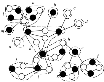
Figure 1: In this bipartite graph $G=(A,B,E)$, $A$ is the set of shaded vertices and $B$ the set of unshaded vertices. The vertices in each block of $G$ are grouped into a dashed circle.

 

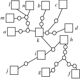
Figure 2: This is the block tree of the graph in Figure 1. The boxes are the latter’s nonsingular blocks and singular pendant ones; the circles are its cut edges and cut vertices.

Lemma 6

1. $\Psi(G)$ is a tree with $O(n)$ vertices. Its leaves are the $|\Lambda(G)|$ pendant blocks of $G$.

2. For all cut vertices $u$ in $G$, ${\cal D}(u,G)$ equals the degree of $u$ in $\Psi(G)$.

Proof: The proof is straightforward and similar to that for similar constructs [9].  

Let $P_{u,v}$ denote the tree path between two vertices $u$ and $v$ in $\Psi(G)$. Let $|P_{u,v}|$ be the number of vertices in $P_{u,v}$.

Lemma 7

Let $Y_{1}$ and $Y_{2}$ be a legal pair of $G$. Let $e$ be a binding edge for $Y_{1}$ and $Y_{2}$. Let $G^{\prime}=G\cup\{e\}$.

1. The cut vertices of $G$ corresponding to c-vertices in $P_{Y_{1},Y_{2}}$ and the vertices of $G$ in the b-vertices on $P_{Y_{1},Y_{2}}$ form a new block $Y_{e}$ in $G^{\prime}$. The b-vertices of $\Psi(G^{\prime})$ are $Y_{e}$ and those of $\Psi(G)$ not on $P_{Y_{1},Y_{2}}$.

2. The c-vertices in $\Psi(G^{\prime})$ are those in $\Psi(G)$ excluding the ones on $P_{Y_{1},Y_{2}}$ that are of degree $2$ in $\Psi(G)$.

3. The edge set of $\Psi(G^{\prime})$ is the union of

   • the set of edges in $\Psi(G)$ whose two endpoints are still in $\Psi(G^{\prime})$;

   • $\{{<\!u,Y_{e}\!>}\mid u\in P_{Y_{1},Y_{2}}$ is a cut vertex of $G$ that remains in $\Psi(G^{\prime})\}$;

   • $\{{<\!u,Y_{e}\!>}\mid u\not\in P_{Y_{1},Y_{2}}$ is a cut vertex of $G$ incident to $P_{Y_{1},Y_{2}}$ in $\Psi(G)\}$.

4. The number of vertices in $\Psi(G^{\prime})$ is at most that for $\Psi(G)$ minus $\frac{|P_{Y_{1},Y_{2}}|-1}{2}$.

5. If $P_{Y_{1},Y_{2}}$ contains a b-vertex of degree at least four in $\Psi(G)$ or two vertices each of degree at least three, then $\Lambda(G^{\prime})=\Lambda(G)-\{Y_{1},Y_{2}\}$.

Proof: The proof is straightforward and similar to those for similar constructs [5, 9, 16, 25].  

A cut vertex $u$ of $G$ is massive if ${\cal D}(u,G)-1>{\cal M}(\Lambda(G))+{\cal R}(\Lambda(G))$; it is critical if ${\cal D}(u,G)-1={\cal M}(\Lambda(G))+{\cal R}(\Lambda(G))$.

Lemma 8

Assume $\Lambda(G)>3$.

1. $G$ has at most two critical vertices. If it has two, then ${\cal R}(\Lambda(G))=0$.

2. $G$ has at most one massive vertex. If it has one, then it has no critical vertex.

Proof: The proof follows from Lemma 6, the inequality ${\cal M}(\Lambda(G))+{\cal R}(\Lambda(G))\geq\frac{|\Lambda(G)|}{2}$, and basic counting arguments for trees.  

The next theorem is the main result of this section.

Theorem 9

${\cal B}(G)\leq\eta(G)$.

Proof: By Lemma 8, we divide the proof into the following five cases. The first case is discussed in Lemma 10; the other cases are proved in §3.1–§3.4, respectively.

Case S1: $|\Lambda(G)|\leq 3$.

Case S2: $|\Lambda(G)|>3$ and ${\cal M}(\Lambda(G))=0$.

Case S3: $|\Lambda(G)|>3$, ${\cal M}(\Lambda(G))>0$, and $G$ has two critical vertices.

Case S4: $|\Lambda(G)|>3$, ${\cal M}(\Lambda(G))>0$, and $G$ has no massive vertex and at most one critical vertex.

Case S5: $|\Lambda(G)|>3$, ${\cal M}(\Lambda(G))>0$, and $G$ has exactly one massive vertex.  

Lemma 10

For Case S1, Theorem 9 holds. Furthermore, given $G$, an optimal biconnector can be computed in $O(m+n)$ time.

Proof: Straightforward.  

3.1 Case S2 of Theorem 9

Lemma 11

Theorem 9 holds for Case S2.

Proof: Let $k=|\Lambda(G)|$. Since ${\cal M}(\Lambda(G))=0$, $\eta(G)=k$ by Lemma 6. It suffices to construct a biconnector $L$ of $k$ edges for $G$. Let $Y_{1},\ldots,Y_{k}$ be the pendant blocks of $G$. Since ${\cal M}(\Lambda(G))=0$, $Y_{i}=\{y_{i}\}$ and we may assume $y_{i}\in B$ without loss of generality. Then, $G$ has a cut edge $(x_{i},y_{i})$ for each $y_{i}$, where $x_{i}\in A$. Since $|A|\geq 2$ and ${\cal M}(\Lambda(G))=0$, there is some $x_{j}\neq x_{1}$. Let $G^{\prime}$ be the connected component of $G-\{x_{1}\}$ containing $x_{j}$. Let $L$ be the set of legal edges $(y_{i},x_{1})$ for all $y_{i}\in G^{\prime}$ and $(y_{i},x_{j})$ for all $y_{i}\not\in G^{\prime}$. It is straightforward to prove that $L$ is as desired by means of Lemma 7.  

3.2 Case S3 of Theorem 9

A path $v_{1},\ldots,v_{k}$ in $\Psi(G)$ is branchless if for all $i$ with $1<i<k$ the degree of $v_{i}$ in $\Psi(G)$ is two. Let $u_{1}$ and $u_{2}$ be the critical vertices of $G$. A leaf clings to $u_{i}$ in $\Psi(G)$ if there is a branchless path between it and $u_{i}$.

Lemma 12

1. $\eta(G)={\cal M}(\Lambda(G))=\frac{|\Lambda(G)|}{2}$.

2. $\Psi(G)$ has a branchless path between $u_{1}$ and $u_{2}$, and exactly $\frac{|\Lambda(G)|}{2}$ leaves cling to $u_{1}$ only while the other $\frac{|\Lambda(G)|}{2}$ leaves cling to $u_{2}$ only.

3. $\Lambda(G)$ has a maximum legal matching in which each legal pair is between one clinging to $u_{1}$ and one clinging to $u_{2}$.

Proof: Statement 1 follows Lemma 8. Statement 2 follows from basic counting arguments for trees. Statement 3 follows from the first two and Lemma 2(1).  

Lemma 13

Theorem 9 holds for Case S3.

Proof: We add to $G$ a binding edge for each legal pair in the maximum legal matching of Lemma 12. By Lemmas 7 and 12, the resulting graph is biconnected. We add $\frac{|\Lambda(G)|}{2}$ edges, which by Lemma 12(1) is optimal.  

3.3 Case S4 of Theorem 9

Since $|\Lambda(G)|>3$, we can divide Case S4 into two subcases:

Case S4-1: $\Psi(G)$ has exactly one vertex of degree at least three.

Case S4-2: $\Psi(G)$ has more than one vertex of degree at least three.

Lemma 14

Theorem 9 holds for Case S4-1.

Proof: Let $x$ be the vertex in $\Psi(G)$ of degree at least three. There are two cases:

Case 1: $x$ is a $b$-vertex. Then, $\eta(G)={\cal R}(\Lambda(G))+{\cal M}(\Lambda(G))$.

Case 2: $x$ is a $c$-vertex. Since $x$ is not massive, $\eta(G)={\cal D}(x,G)-1={\cal R}(\Lambda(G))+{\cal M}(\Lambda(G))$ and ${\cal M}(\Lambda(G))=1$.

In either case, let $N_{1}$ be a maximum legal matching of $\Lambda(G)$; next, let $N_{2}$ be a set of legal pairs formed by pairing each pendant block not yet matched in $N_{1}$ with one already matched. Then, $N=N_{1}\cup N_{2}$ is a set of the smallest number of legal pairs of $G$ such that each element in $\Lambda(G)$ is in a pair. We add to $G$ a binding edge for each pair in $N$. Since ${\cal M}(\Lambda(G))>0$, we add $\eta(G)$ edges. Since ${\cal M}(\Lambda(G))>0$ in Case 1 and ${\cal M}(\Lambda(G))=1$ in Case 2, these edges form a desired biconnector by Lemma 7.  

To discuss Case S4-2, we further assume that $\Psi(G)$ is rooted at a vertex with at least two neighbors; however, the degree of a vertex in $\Psi(G)$ still refers to its number of neighbors instead of children.

The next lemma chooses an advantageous root for $\Psi(G)$ for our augmentation algorithm. Given a vertex $v$ in $\Psi(G)$, a branch of $v$, also called a $v$-branch, is the subtree of $\Psi(G)$ rooted at a child of $v$. A chain of $v$, also called a $v$-chain, is a $v$-branch that contains exactly one leaf in $\Psi(G)$.

Let $c^{*}$ be a c-vertex in $\Psi(G)$ of the largest possible degree.

Lemma 15

In Case S4-2, we can reroot $\Psi(G)$ at a vertex $h$ such that

1. either $h$ is of degree two and no $h$-branch is a chain or $h$ is of degree at least three;

2. if $c^{*}$ is critical, then $h=c^{*}$.

Proof: Let $r$ be the current root of $\Psi(G)$. There are three cases.

Case 1: $c^{*}$ is not critical, and either $r$ is of degree two and no $r$-branch is a chain or $r$ is of degree at least three. We set $h=r$.

Case 2: $c^{*}$ is not critical, $r$ is of degree two, and an $r$-branch is a chain. Note that $\Psi(G)$ has a vertex $r^{*}$ of degree at least three. We set $h=r^{*}$.

Case 3: $c^{*}$ is critical. Since $|\Lambda(G)|>3$, $c^{*}$ is of degree three or more. We set $h=c^{*}$.  

Lemma 16

Let $h$ be the root of $\Psi(G)$. In Case S4-2, if either $h$ is of degree two and no $h$-branch is a chain or $h$ is of degree at least three, then $G$ has a legal pair $w_{1}$ and $w_{2}$ such that

1. $P_{w_{1},w_{2}}$ passes through $h$ and two vertices of degree at least three;

2. ${\cal M}(\Lambda(G)-\{w_{1},w_{2}\})={\cal M}(\Lambda(G))-1$.

Proof: There are two cases.

Case 1: The degree of $h$ is two and no $h$-branch is a chain. Let $T^{*}$ be an $h$-branch.

Case 2: The degree of $h$ is at least three. Since this is Case S4-2, some descendant of $h$ has degree at least three. Let $T^{*}$ be the $h$-branch containing that descendant.

Let $W_{1}$ be the set of leaves in $T^{*}$. Let $W_{2}=\Lambda(G)-W_{1}$. By Lemma 2(1), there exist a legal pair $w_{1}\in W_{1}$ and $w_{2}\in W_{2}$ with ${\cal M}(\Lambda(G)-\{w_{1},w_{2}\})={\cal M}(\Lambda(G))-1$. Then, $P_{w_{1},w_{2}}$ contains $h$ as desired. Furthermore, in Case 1, $P_{w_{1},w_{2}}$ contains a vertex of degree at least three in $T^{*}$ and another in $\Psi(G)-T^{*}$; in Case 2, $h$ itself is of degree at least three, and $P_{w_{1},w_{2}}$ contain a vertex of degree at least three in $T^{*}$. In both cases, $P_{w_{1},w_{2}}$ is as desired.  

Lemma 17

In Case S4-2, we can add a legal edge to $G$ such that

1. the resulting graph $G^{\prime}$ satisfies Case S1, S2, S3 or S4;

2. $\eta(G^{\prime})=\eta(G)-1$;

3. if $G$ has a critical vertex, then that vertex remains critical in $G^{\prime}$.

Proof: We use Lemma 15 to reroot $\Psi(G)$, use Lemma 16 to pick a legal pair $w_{1}$ and $w_{2}$, and then add a binding edge for this pair to $G$. By Lemmas 16(1) and 7(5), $\Lambda(G^{\prime})=\Lambda(G)-\{w_{1},w_{2}\}$. By Lemma 16(2), ${\cal M}(\Lambda(G^{\prime}))={\cal M}(\Lambda(G))-1$. Hence ${\cal M}(\Lambda(G^{\prime}))+{\cal R}(\Lambda(G^{\prime}))={\cal M}(\Lambda(G))+{\cal R}(\Lambda(G))-1$. There are two cases.

Case 1: $G$ has no critical vertex. Then, by Lemma 7, $\max_{u\in G^{\prime}}{\cal D}(u,G^{\prime})\leq\max_{u\in G}$ ${\cal D}(u,G)\leq{\cal M}(\Lambda(G))+{\cal R}(\Lambda(G))$.

Case 2: $G$ has a critical vertex. Then, $c^{*}$ is the critical vertex and ${\cal D}(c^{*},G)>\max_{u\neq c^{*}}{\cal D}(u,G)$. By Lemmas 15(2), 16(1), and Lemma 7, $\max_{u\in G^{\prime}}{\cal D}(u,G^{\prime})=\max_{u\in G}$ ${\cal D}(u,G)-1={\cal M}(\Lambda(G))+{\cal R}(\Lambda(G))$. Hence $c^{*}$ remains to be a critical vertex.

In either case, $\max_{u\in G^{\prime}}{\cal D}(u,G^{\prime})-1\leq{\cal M}(\Lambda(G^{\prime}))+{\cal R}(\Lambda(G^{\prime}))$. Then, $\eta(G^{\prime})=\eta(G)-1$. Also, $G^{\prime}$ has no massive vertex and thus satisfies Case S1, S2, S3 or S4.  

Lemma 18

Theorem 9 holds for Case S4.

Proof: For Case S4-1, we use Lemma 14. For Case S4-2, we add one edge to $G$ at a time using Lemma 17 until the resulting graph $G^{\prime}$ does not satisfy Case S4-2. By Lemma 17(1), $G^{\prime}$ satisfies Case S1, S2, S3 or S4-1. Thus, we apply Lemma 10, 11, 13, or 14 to $G^{\prime}$ accordingly. By Lemma 17(2), the number of edges added is $\eta(G)$.  

3.4 Case S5 of Theorem 9

Let $r$ be the massive cut vertex of $G$. Let $\Psi(G)$ be rooted at $r$.

Lemma 19

1. $\eta(G)={\cal D}(r,G)-1>{\cal M}(\Lambda(G))+{\cal R}(\Lambda(G))>{\cal D}(u,G)-1$ for any vertex $u\neq r$.

2. ${\cal D}(r,G)\geq 4$ and there are at least four $r$-chains.

3. The tree $\Psi(G)$ contains a legal pair $Y_{1}$ and $Y_{2}$ as well as two distinct $r$-branches $T_{1}$ and $T_{2}$ such that $T_{1}$ is a chain, $Y_{1}\in T_{1}$, and $Y_{2}\in T_{2}$.

Proof:

Statement 1. This statement follows from the definition of Case S5.

Statement 2. Let $\delta_{1}$ be the number of $r$-chains. Then, ${\cal D}(r,G)\geq\delta_{1}$ and $|\Lambda(G)|\geq 2({\cal D}(r,G)-\delta_{1})+\delta_{1}$. So ${\cal D}(r,G)\geq\delta_{1}\geq 2{\cal D}(r,G)-|\Lambda(G)|$. Let $\delta_{2}=({\cal D}(r,G)-1)-({\cal M}(\Lambda(G))+{\cal R}(\Lambda(G)))$. Because $r$ is massive, $\delta_{2}\geq 1$. Note that $|\Lambda(G)|=2{\cal M}(\Lambda(G))+{\cal R}(\Lambda(G))$. Thus ${\cal D}(r,G)\geq\delta_{1}\geq 2\delta_{2}+2+{\cal R}(\Lambda(G))\geq 4$.

Statement 3. Let $T_{1}$ be an $r$-chain. Let $Y_{1}$ be the leaf of $\Psi(G)$ in $T_{1}$. Because ${\cal M}(\Lambda(G))>0$, $\Psi(G)$ contains a leaf $Y_{2}\neq Y_{1}$ that forms a legal pair with $Y_{1}$. Let $T_{2}$ be the $r$-branch that contains $Y_{2}$. Then, $Y_{1}$, $Y_{2}$, $T_{1}$ and $T_{2}$ are as desired.  

Lemma 20

We can add a legal edge to $G$ such that for the resulting graph $G^{\prime}$,

1. $\eta(G^{\prime})=\eta(G)-1$;

2. ${\cal D}(r,G^{\prime})={\cal D}(r,G)-1$.

Proof: Let $Y_{1}$, $Y_{2}$, $T_{1}$ and $T_{2}$ be as stated in Lemma 19(3). The added edge is a binding edge for $Y_{1}$ and $Y_{2}$. By Lemma 7, the b-vertices and c-vertices on $P_{Y_{1},Y_{2}}$ form a new block $Y^{\prime}$ in $G^{\prime}$. $Y^{\prime}$ may or may not be a leaf in $\Psi(G^{\prime})$; in either case, ${\cal M}(\Lambda(G^{\prime}))+{\cal R}(\Lambda(G^{\prime}))\leq{\cal M}(\Lambda(G))+{\cal R}(\Lambda(G))$. Note that $P_{Y_{1},Y_{2}}$ contains $r$. Thus, by Lemmas 7 and 19(2), $r$ remains a cut vertex in $G^{\prime}$ with ${\cal D}(r,G^{\prime})={\cal D}(r,G)-1$ while ${\cal D}(v,G^{\prime})\leq{\cal D}(v,G)$ for all vertices $v\neq r$. Consequently, $\eta(G^{\prime})=\eta(G)-1$.  

Lemma 21

Theorem 9 holds for Case S5. Moreover, this case can be reduced in linear time to Case S1, S2, S3 or S4.

Proof: We add one edge to $G$ at a time using Lemma 20 until the resulting graph $G^{\prime}$ satisfies Case S1, S2, S3 or S4. Thus, we apply Lemma 10, 11, 13 or 18 accordingly. By Lemma 20(1), $\eta(G)$ edges are added. To implement this proof in linear time, we first define a data structure as follows.

Let $Q$ be the set of leaves of $\Psi(G)$ that are in the $r$-chains. We set up a counter for the number of these leaves. We also set up three doubly linked lists containing those of them that are types $A$, $B$, and $AB$, respectively.

We set up a counter for the number of $r$-branches that are not chains. For each such branch, we set up a doubly linked list for the leaves of $\Psi(G)$ in it. We also set up three doubly linked lists for the leaves in these branches that are types $A$, $B$, and $AB$, respectively.

Given $G$, we can set up these linked lists and counters in linear time. We next use this data structure to find a legal pair $Y_{1}$ and $Y_{2}$ by means of Lemma 19(3). Since $|Q|\geq 4$ by Lemma 19(2), there are two cases.

Case 1: Some $Y_{1}$ and $Y_{2}\in Q$ form a legal pair. This is our desired pair. Note the $r$-chains containing $Y_{1}$ and $Y_{2}$ in $\Psi(G)$ are contracted into a new chain in $\Psi(G^{\prime})$ consisting of a single leaf of type $AB$.

Case 2: $Q$ contains only type $A$ or $B$ leaves. Select any $Y_{1}\in Q$. Since ${\cal M}(\Lambda(G))>0$, some $Y_{2}\in\Lambda(G)-Q$ forms a desire legal pair with $Y_{1}$. Note that $Y_{1}$ and $Y_{2}$ are no longer pendant blocks in $G^{\prime}$ and the newly created block is not a pendant block of $G^{\prime}$, either. The $r$-branch containing $Y_{2}$ becomes a chain if in $G$ it contains exactly two pendant blocks.

It takes $O(1)$ time to decide which of these two cases holds. In either case, the selection of $Y_{1}$ and $Y_{2}$ takes in $O(1)$ time using the linked lists. Once $Y_{1}$ and $Y_{2}$ are found, we can find a binding edge in $O(1)$ time in a straightforward manner. After the edge is added to $G$, we can update the data structure in $O(1)$ time for $G^{\prime}$. Then, we use Lemma 2(2) and the counters to check whether $G^{\prime}$ satisfies Case S5 in $O(1)$ time. We repeat this process until $G^{\prime}$ does not satisfies Case S5. At this point, we complete the reduction. Since we iteratively add at most $O(n)$ edges in Case S5, the reduction takes linear time.  

4 Computing an optimal biconnector in linear time

Theorem 22

Given $G$, an optimal biconnector is computable in $O(m+n)$ time.

We prove this theorem by means of Theorems 5 and 9 as follows.

Given $G$, it takes $O(m+n)$ time to determine which case of Theorem 5 holds. Then, it takes $O(m+n)$ time in a straightforward manner to compute an optimal biconnector for Cases M2, M4, M5 and M6; reduce Case M3 to Case M1 or M2; and reduce Case M1 to Theorem 9.

Next, it takes $O(m+n)$ time to determine which case of Theorem 9 holds. Then, it is straightforward to compute an optimal biconnector in $O(m+n)$ time for Cases S1, S2, and S3. Lemma 21 reduces Case S5 in $O(m+n)$ time to Case S1, S2, S3 or S4. By Lemma 14, we can find an optimal biconnector in $O(m+n)$ time for Case S4-1. The remaining proof shows how to reduce Case S4-2 to Case S1, S2, S3 or S4-1 in $O(m+n)$ time by implementing the proof of Lemma 18.

We define a data structure $\Delta(G)$ as follows. First, we root $\Psi(G)$ at a vertex of degree two or more as in §3.3 and classify each vertex $u$ by a 4-bit code $\sigma_{0}\sigma_{1}\sigma_{2}\sigma_{3}$ based on the subtree $T_{u}$ of $\Psi(G)$ rooted at $u$:

• $\sigma_{0}=1$ if and only if $T_{u}$ has more than one leaf;

• $\sigma_{1}$, $\sigma_{2}$ or $\sigma_{3}=1$ if and only if $T_{u}$ contains a leaf of type $A$, $B$ or $AB$, respectively.

The code has at most ten combinations, i.e., $0100$, $0010$, $0001$ and all the combinations with $\sigma_{0}=1$ except $1000$. $\Delta(G)$ is $\Psi(G)$ augmented with the following items:

1. At each vertex in $\Psi(G)$, $\Delta(G)$ maintains its degree and a doubly linked list for the children of $u$ with the same $\sigma_{0}\sigma_{1}\sigma_{2}\sigma_{3}$ code. There are ten such lists.

2. There are three counters for the numbers of leaves in $\Psi(G)$ of types $A$, $B$ and $AB$, respectively.

3. The c-vertices of degree at least three are partitioned into groups of the same degree. Each nonempty group is arranged into a doubly linked list. The lists themselves are connected by a doubly linked list in the increasing order of vertex degrees.

We do not need parent pointers in $\Delta(G)$, which are subtle to update [15, 16, 25]. This finishes the description of $\Delta(G)$. We can build $\Delta(G)$ from $G$ in $O(m+n)$ time.

Lemma 23

1. Let $r$ be the current root of $\Delta(G)$. Let $h$ be as stated in Lemma 15. Given $\Delta(G)$, if $r$ is critical, we can reroot $\Delta(G)$ in $O(1)$ time according to Lemma 15; $O(n)$ time if $r$ is not critical but $h$ is; or $O(|P_{r,h}|)$ time if neither is.

2. Given $\Delta(G)$, we can find $w_{1}$ and $w_{2}$ of Lemma 16 in $O(|P_{w_{1},w_{2}}|)$ time.

Proof:

Statement 1. We implement the proof Lemma 15 using the following steps.

1. Use Item 3 of $\Delta(G)$ to find $c^{*}$.

2. Use Items 1 and 2 of $\Delta(G)$ and Lemma 2(2) to decide which case of the proof of Lemma 15 holds.

3. 1. For Case 1 of the proof of Lemma 15, set $h=r$ and $\Delta(G)$ is unchanged.

   2. For Case 2 of the proof of Lemma 15, first use Item 1 of $\Delta(G)$ to find the nearest desired descendant $r^{*}$ of $r$ and then reroot $\Delta(G)$ at $h=r^{*}$ and update it accordingly.

   3. For Case 3 of the proof of Lemma 15, if $r\neq c^{*}$, then recompute $\Delta(G)$ from $\Psi(G)$ to root at $h=c^{*}$; otherwise, $r=c^{*}$, and $\Delta(G)$ is unchanged.

Since Steps 1 and 2 take $O(1)$ time, the the time complexity of each case of this statement is bounded by that of Step 3.

Case 1: $r$ is critical. Step 3c runs with $r=c^{*}$ in $O(1)$ time.

Case 2: $r$ is not critical but $h$ is. Step 3c runs with $r\neq c^{*}$ in $O(n)$ time.

Case 3: Neither $r$ nor $h$ is critical. Then, Step 3a or Step 3b is performed. Step 3a takes $O(1)$ time. For Step 3b, the search for $r^{*}$ takes $O(1)$ time per vertex on $P_{r,r^{*}}$. Since the internal vertices of $P_{r,r^{*}}$ all have degree two, updating Item 1 of $\Delta(G)$ along this path takes $O(1)$ time per vertex. Item 1 of $\Delta(G)$ outside this path and the other two items remain the same. Thus, this case takes $O(P_{r,h})$ total time as desired.

Statement 2. We implement the proof of Lemma 16 using the following steps.

1. Use Item 1 of $\Delta(G)$ to decide which case of the proof of Lemma 16 holds.

2. Use Item 2 of $\Delta(G)$ and Lemma 2(2) to find all possible pairs of types $t_{1}$ and $t_{2}$ such that $\Lambda(G)$ has a maximum matching that contains a legal pair between type $t_{1}$ and type $t_{2}$.

3. For each such pair of $t_{1}$ and $t_{2}$, perform the following computation until $w_{1}$ and $w_{2}$ are found.

   1. For Case 1 of the proof of Lemma 16, $w_{1}$ and $w_{2}$ are in the two branches of the root of $\Delta(G)$ separately. Use Item 1 of $\Delta(G)$ at the root to decide whether the desired $w_{1}$ and $w_{2}$ exist. If they exist, use Item 1 of $\Delta(G)$ to search for them.

   2. For Case 2 of the proof of Lemma 16, $w_{1}$ and $w_{2}$ are in two separate branches of the root, of which one is not a chain. The remaining computation is similar to that of Step 3a.

By Lemma 15, some pair $t_{1}$ and $t_{2}$ yields the desired $w_{1}$ and $w_{2}$. Steps 1 and 2 take $O(1)$ time. There are $O(1)$ possible pairs of $t_{1}$ and $t_{2}$. For each such pair, checking the existence of $w_{1}$ and $w_{2}$ takes $O(1)$ time. If they exist, searching for them takes $O(1)$ time per vertex on the path $P_{w_{1},w_{2}}$.  

The next lemma completes the proof of Theorem 22.

Lemma 24

Case S4-2 is reducible to Case S1, S2, S3 or S4-1 in $O(m+n)$ time.

Proof: Given $G$ in Case S4-2 as input, the reduction algorithm is as follows:

1. Construct $\Delta(G)$.

2. repeat

   1. Use Lemma 23(1) to reroot $\Delta(G)$.

   2. Use Lemma 23(2) to find a legal pair $w_{1}$ and $w_{2}$.

   3. Add a binding edge $e$ for $w_{1}$ and $w_{2}$ into $G$.

   4. Use Lemma 7 to update $\Delta(G)$ while rerooting it at the new b-vertex $Y_{e}$ resulting from the insertion of $e$.

   until $G$ does not satisfy Case S4-2.

Since Step 1 takes $O(m+n)$ time, it suffices to prove that Step 2 takes $O(n)$ time. By Lemma 16(1), each iteration of Step 2 reduces $|\Lambda(G)|$ by two. Since $|\Lambda(G)|<n$, the repeat loop has less than $n$ iterations. Then, since the until condition can be checked in $O(1)$ time per iteration using Lemma 2(2) and Items 2 and 3 of $\Delta(G)$, the until step takes $O(n)$ total time. Similarly, Step 2c takes $O(1)$ time per iteration and $O(n)$ total time in a straightforward manner.

We next show that Steps 2a, 2b and 2d also take $O(n)$ total time. For a given iteration, let $G_{0}$ and $G_{1}$ denote $G$ before and after $e$ is inserted, respectively.

Step 2a. We show that each case in the proof of Lemma 23(1) takes $O(n)$ total time as follows.

Case 1. This case takes $O(1)$ time per iteration and thus $O(n)$ total time.

Case 2. By Lemma 17(3), this case can only happen once in the above augmentation algorithm. Hence, this case takes $O(n)$ total time.

Case 3. This case takes $O(1)$ time per edge on $P_{r,h}$ for an iteration. Note that the degree of a vertex in $\Delta(G)$ never increases by edge insertion. Then, since $\Delta(G_{1})$ is rooted at $Y_{e}$ with $e$ connecting two leaves of $\Delta(G_{0})$, each edge on $P_{r,h}$ is traversed only once to reroot $\Delta(G)$ for this case throughout all the iterations. Therefore, this case takes $O(n)$ total time.

Step 2b. This step takes $O(|P_{w_{1},w_{2}}|)$ time per iteration. Since there are $O(n)$ iterations, by Lemma 7(4), this step takes $O(n)$ total time.

Step 2d. We bound the time for updating each item of $\Delta(G)$ as follows.

Item 1 of $\Delta(G)$. Notice that $P_{w_{1},w_{2}}$ passes through the root of $\Delta(G_{0})$. Also, $\Delta(G_{1})$ is rooted at $Y_{2}$. These properties make it straightforward to update this item in $O(|P_{w_{1},w_{2}}|)$ time per iteration. Since there are $O(n)$ iterations, by Lemma 7(4), this step takes $O(n)$ total time.

Item 2 of $\Delta(G)$. By Lemma 16(1), $\Lambda(G_{1})=\Lambda(G_{0})-\{w_{1},w_{2}\}$. Thus it takes $O(1)$ time to update this item per iteration and $O(n)$ total time.

Item 3 of $\Delta(G)$. Let $u$ be a c-vertex in $\Delta(G_{0})$. If $u\not\in P_{w_{1},w_{2}}$, it has the same degree in $\Delta(G_{0})$ and $\Delta(G_{1})$ and is not relocated in this item. If $u\in P_{w_{1},w_{2}}$, its degree reduces at most 2 in $\Delta(G_{1})$ and can be relocated in $O(1)$ time. Therefore, this item can be updated in $O(|P_{w_{1},w_{2}}|)$ time per iteration, i.e., $O(n)$ total time as shown for Item 1.

References

- [1] N. R. Adam and J. C. Wortmann, Security-control methods for statistical database: A comparative study, ACM Computing Surveys, 21 (1989), pp. 515–556.
- [2] F. Y. Chin and G. Özsoyoğlu, Auditing and inference control in statistical databases, IEEE Transactions on Software Engineering, 8 (1982), pp. 574–582.
- [3] L. H. Cox, Suppression methodology and statistical disclosure control, Journal of the American Statistical Association, Theory and Method Section, 75 (1980), pp. 377–385.
- [4] D. E. Denning and J. Schlörer, Inference controls for statistical databases, IEEE Transactions on Computers, (1983), pp. 69–82.
- [5] K. P. Eswaran and R. E. Tarjan, Augmentation problems, SIAM Journal on Computing, 5 (1976), pp. 653–665.
- [6] A. Frank, Augmenting graphs to meet edge-connectivity requirements, SIAM Journal on Discrete Mathematics, 5 (1992), pp. 25–43.
- [7] , Connectivity augmentation problems in network design, in Mathematical Programming: State of the Art 1994, J. R. Birge and K. G. Murty, eds., The University of Michigan, 1994, pp. 34–63.
- [8] D. Gusfield, A graph theoretic approach to statistical data security, SIAM Journal on Computing, 17 (1988), pp. 552–571.
- [9] F. Harary, Graph Theory, Addison-Wesley, Reading, MA, 1969.
- [10] T.-s. Hsu, On four-connecting a triconnected graph extended abstract, in Proceedings of the 33rd Annual IEEE Symposium on Foundations of Computer Science, 1992, pp. 70–79.
- [11] , Graph augmentation and related problems: Theory and practice, Ph.D. thesis, University of Texas at Austin, 1993.
- [12] , Undirected vertex-connectivity structure and smallest four-vertex-connectivity augmentation extended abstract, in Lecture Notes in Computer Science 1004: Proceedings of the 6th Annual International Symposium on Algorithms and Computation, J. Staples, ed., New York, NY, 1995, Springer-Verlag, pp. 274–283.
- [13] T.-s. Hsu and M. Y. Kao, Optimal bi-level augmentation for selectively enhancing graph connectivity with applications, in Lecture Notes in Computer Science 1090: Proceedings of the 2nd Annual International Computing and Combinatorics Conference, J. Y. Cai and C. K. Wong, eds., Springer-Verlag, New York, NY, 1996, pp. 169–178.
- [14] , Security problems for statistical databases with general cell suppressions, in Proceedings of the 9th International Conference on Scientific and Statistical Database Management, D. Hansen and Y. Ioannidis, eds., IEEE Computer Society, Washington, DC, 1997, pp. 155–164.
- [15] T.-s. Hsu and V. Ramachandran, A linear time algorithm for triconnectivity augmentation, in Proceedings of the 32nd Annual IEEE Symposium on Foundations of Computer Science, 1991, pp. 548–559.
- [16] , On finding a smallest augmentation to biconnect a graph, SIAM Journal on Computing, 22 (1993), pp. 889–912.
- [17] G. Kant, Algorithms for drawing planar graphs, Ph.D. thesis, Utrecht University, the Netherlands, 1993.
- [18] M. Y. Kao, Linear-time optimal augmentation for componentwise bipartite-completeness of graphs, Information Processing Letters, (1995), pp. 59–63.
- [19] , Data security equals graph connectivity, SIAM Journal on Discrete Mathematics, 9 (1996), pp. 87–100.
- [20] , Total protection of analytic-invariant information in cross-tabulated tables, SIAM Journal on Computing, 26 (1997), pp. 231–242.
- [21] J. P. Kelly, B. L. Golden, and A. A. Assad, Cell suppression: Disclosure protection for sensitive tabular data, Networks, 22 (1992), pp. 397–417.
- [22] F. M. Malvestuto and M. Moscarini, Censoring statistical tables to protect sensitive information: Easy and hard problems, in Proceedings of the 8th International Conference on Scientific and Statistical Database Management, 1996, pp. 12–21.
- [23] , Suppressing marginal totals from a two-dimensional table to protect sensitive information, Statistics and Computing, 7 (1997), pp. 101–114.
- [24] F. M. Malvestuto, M. Moscarini, and M. Rafanelli, Suppressing marginal cells to protect sensitive information in a two-dimensional statistical table, in Proceedings of the 3rd ACM Symposium on Principles of Database Systems, 1991, pp. 252–258.
- [25] A. Rosenthal and A. Goldner, Smallest augmentations to biconnect a graph, SIAM Journal on Computing, 6 (1977), pp. 55–66.
- [26] S. Taoka and T. Watanabe, Minimum augmentation to -edge-connect specified vertices of a graph, in Lecture Notes in Computer Science 834: Proceedings of the 5th Annual International Symposium on Algorithms and Computation, D. Z. Du and X. S. Zhang, eds., Springer-Verlag, New York, NY, 1994, pp. 217–225.
- [27] T. Watanabe, Y. Higashi, and A. Nakamura, An approach to robust network construction from graph augmentation problems, in Proceedings of the 1990 IEEE International Symposium on Circuits and Systems, 1990, pp. 2861–2864.
- [28] , Graph augmentation problems for a specified set of vertices, in Lecture Notes in Computer Science 450: Proceedings of the 1st Annual International Symposium on Algorithms, T. Asano, T. Ibaraki, H. Imai, and T. Nishizeki, eds., Springer-Verlag, New York, NY, 1990, pp. 378–387.
- [29] T. Watanabe and A. Nakamura, A minimum 3-connectivity augmentation of a graph, Journal of Computer and System Sciences, 46 (1993), pp. 91–128.
- [30] T. Watanabe, S. Taoka, and T. Mashima, Minimum-cost augmentation to 3-edge-connect all specified vertices in a graph, in Proceedings of the 1993 IEEE International Symposium on Circuits and Systems, 1993, pp. 2311–2314.