Common-Face Embeddings of Planar Graphs

Abstract

Given a planar graph ${\cal G}$ and a sequence ${{\cal C}}_{1},\ldots,{{\cal C}}_{q}$, where each ${{\cal C}}_{i}$ is a family of vertex subsets of ${\cal G}$, we wish to find a plane embedding of ${\cal G}$, if any exists, such that for each $i\in\{1,\ldots,q\}$, there is a face $F_{i}$ in the embedding whose boundary contains at least one vertex from each set in ${\cal C}_{i}$. This problem has applications to the recovery of topological information from geographical data and the design of constrained layouts in VLSI. Let $I$ be the input size, i.e., the total number of vertices and edges in ${\cal G}$ and the families ${{\cal C}}_{i}$, counting multiplicity. We show that this problem is NP-complete in general. We also show that it is solvable in $O(I\log I)$ time for the special case where for each input family ${{\cal C}}_{i}$, each set in ${{\cal C}}_{i}$ induces a connected subgraph of the input graph ${\cal G}$. Note that the classical problem of simply finding a planar embedding is a further special case of this case with $q=0$. Therefore, the processing of the additional constraints ${{\cal C}}_{1},\ldots,{{\cal C}}_{q}$ only incurs a logarithmic factor of overhead.

1 Introduction

It is a fundamental problem in mathematics (e.g., see [13, 17, 18, 19, 20, 29]) to embed a graph into a given surface while optimizing certain objectives required by applications. (Throughout this paper, a graph may have multiple edges and selfloops but a simple graph always has neither.) A graph is planar if it can be embedded on the plane so that any pair of edges can only intersect at their endpoints; a plane graph is a planar one together with such an embedding. A classical variant of the problem is to test whether a given graph is planar and in case it is, to find a planar embedding. This planarity problem can be solved in linear time sequentially [4, 5, 19] and efficiently in parallel [26].

In this paper, we initiate the study of the following new planarity problem. Let ${\cal G}$ be a planar graph. Let ${\cal M}$ be a sequence ${{\cal C}}_{1},\ldots,{{\cal C}}_{q}$, where each ${{\cal C}}_{i}$ is a family of vertex subsets of ${\cal G}$. A plane embedding ${\Phi}$ of ${\cal G}$ satisfies ${\cal C}_{i}$ if the boundary of some face in ${\Phi}$ contains at least one vertex from each set in ${\cal C}_{i}$. ${\Phi}$ satisfies ${\cal M}$ if it satisfies all ${\cal C}_{i}$. ${\cal G}$ satisfies ${\cal M}$ if ${\cal G}$ has an embedding that satisfies ${\cal M}$.

Problem 1 (the common-face embedding (CFE) problem)

• Input: A planar graph ${\cal G}$ and a sequence ${\cal M}$ of families of vertex subsets of ${\cal G}$.

• Question: Does ${\cal G}$ satisfy ${\cal M}$?

Let $I$ be the input size, i.e., the total number of vertices and edges in ${\cal G}$ and the families ${\cal C}_{i}$, counting multiplicity. We first show that the CFE problem is NP-complete in general. Then, for the special case where each vertex subset in each ${\cal C}_{i}$ induces a connected subgraph of ${\cal G}$, we give an $O(I\log{I})$-time algorithm which can actually find a plane embedding satisfying ${\cal M}$, if any exists. Note that the classical problem of simply finding a planar embedding is a further special case of this special case with $q=0$. Therefore, the processing of the additional constraints ${{\cal C}}_{1},\ldots,{{\cal C}}_{q}$ only incurs a logarithmic factor of overhead.

The CFE problem arises naturally from topological inference [6]. For instance, in the conference version of this paper [7], a less general and less efficient variant of our algorithm for the special case has been employed to design fast algorithms for reconstructing maps from scrambled partial data in geometric information systems [7]. In this application [8, 9, 10, 15, 23, 24], each vertex subset in ${\cal M}$ describes a recognizable geographical feature and each face in a planar embedding represents a geographical region. Each family in ${\cal M}$ is a set of features that are known to be near each other, i.e., surrounding the same region (on the boundary of the same face). Similarly, our algorithm for the special case can compute a constrained layout of VLSI modules [14], where each vertex subset consists of the ports of a module, and each subset family specifies a set of modules that are required to be close to each other [7].

To the best of our knowledge, the conference version of this paper is the first to investigate the CFE problem [7]. A related problem has been studied in the context of speeding up the computation of Steiner trees and minimum-concave-cost network flows [11, 25, 3]. Given a planar graph $G=(V,E)$ and a set of special vertices $S\subseteq V$, the pair $(G,S)$ is called $k$-planar if all the vertices in $S$ are on the boundaries of at most $k$ faces of a planar embedding of $G$. Bienstock and Monma [3] showed that testing $k$-planarity is NP-complete if $k$ is part of the input but takes linear time for any fixed $k$.

The remainder of this paper is organized as follows. Section 2 proves the NP-completeness result and formally states the main theorem on the CFE algorithm (Theorem 2.2). Sections 3 through 6 prove the main theorem by detailing the algorithm for the key cases where ${\cal G}$ is (1) triconnected, (2) disconnected, (3) connected, or (4) biconnected, respectively. The triconnected case is the base case in that the other cases are eventually reduced to it. For this reason, this case is analyzed before the other cases. Section 7 concludes this paper with some directions for further research.

2 Basics and the main results

2.1 Basic definitions

Let $G$ be a graph. $|G|$ denotes the size of $G$, i.e., the total number of vertices and edges in $G$. ${\cal V}(G)$ denotes the vertex set of $G$. If $G$ is a plane graph, then ${\cal F}(G)$ denotes the set of faces of $G$.

A set $U$ is $G$-local if $U\subseteq{\cal V}(G)$. A family ${\cal C}$ of sets is $G$-local if every set in ${\cal C}$ is $G$-local.

For a subset $U$ of ${\cal V}(G)$, the subgraph of $G$ induced by $U$ is the graph $(U,E_{U})$ where $E_{U}$ consists of all edges $e$ of $G$ whose endpoints both belong to $U$; $G-U$ denotes the subgraph of $G$ induced by ${\cal V}(G)-U$.

A cut vertex of $G$ is one whose removal increases the number of connected components in $G$; a block of $G$ is a maximal subgraph of $G$ with no cut vertex. Let $\Psi(G)$ denote the forest whose vertices are the cut vertices and the blocks of $G$ and whose edges are those $\{v,B\}$ such that $v$ is a cut vertex of $G$, $B$ is a block of $G$, and $v\in{\cal V}(B)$. Note that $\Psi(G)$ is a tree if $G$ is connected.

$G$ is biconnected if it is connected and it has at least two vertices but no cut vertex. $G$ is triconnected if it is biconnected, it has at least three vertices, and the removal of any two vertices cannot disconnect it.

The size of a set $S$, denoted by $|S|$, is the number of elements in $S$. The size of a family ${\cal C}$ of sets, denoted by $|{\cal C}|$, is $\sum_{S}|S|$ where $S$ ranges over all sets in ${\cal C}$. The size of a sequence ${\cal M}$ of families of sets, denoted by $|{\cal M}|$, is $\sum_{{\cal C}}|{\cal C}|$ where ${\cal C}$ ranges over all families in ${\cal M}$.

2.2 An NP-completeness result

Theorem 2.1

The CFE problem is NP-complete.

Proof. We reduce the SATISFIABILITY problem [14] to the CFE problem. Let $\phi$ be a CNF formula over variables $x_{1},\ldots,x_{n}$ with $n\geq 2$. Let $C_{1},\ldots,C_{m}$ be the clauses of $\phi$, each regarded as the set of literals in it. We construct a simple biconnected planar graph ${\cal G}=(V_{1}\cup V_{2},E)$ as follows. $V_{1}=\{x_{1},\ldots,x_{n}\}\cup\{\bar{x}_{1},\ldots,\bar{x}_{n}\}\cup\{c_{1},\ldots,c_{m}\}$. $V_{2}=\{u_{0},\ldots,u_{n}\}$. For each $x_{i}$, ${\cal G}$ contains edges $\{u_{i-1},x_{i}\}$, $\{x_{i},u_{i}\}$, $\{u_{i-1},\bar{x}_{i}\}$, $\{\bar{x}_{i},u_{i}\}$. The only other edges of ${\cal G}$ are $\{u_{0},c_{1}\}$, $\{c_{1},c_{2}\}$, $\{c_{2},c_{3}\}$, …, $\{c_{m-1},c_{m}\}$, $\{c_{m},u_{n}\}$, $\{u_{n},u_{0}\}$. Let ${\cal M}$ be the sequence $\{\{c_{1}\},C_{1}\},\ldots,\{\{c_{m}\},C_{m}\}$. Observe that in every plane embedding ${\Phi}$ of ${\cal G}$, (1) the cycle $c_{1},\ldots,c_{m},u_{n},u_{0}$ forms the boundary of some face $F$ and (2) for $i=1,\ldots,n$, exactly one of $x_{i}$ and $\bar{x}_{i}$ is on the boundary of the face other than $F$ whose boundary contains the path $c_{1},\ldots,c_{m}$. Also, for every set $S\subseteq\{x_{1},\ldots,x_{n}\}\cup\{\bar{x}_{1},\ldots,\bar{x}_{n}\}$ with $|S\cap\{x_{i},\bar{x}_{i}\}|=1$ for all $i=1,\ldots,n$, ${\cal G}$ has a plane embedding where the boundary of some face contains the path $c_{1},\ldots,c_{m}$ and the vertices in $S$. Therefore, $\phi$ is satisfiable if and only if ${\cal G}$ satisfies ${\cal M}$.     

2.3 The main theorem

Although the input to the CFE problem is a planar graph ${\cal G}$, it is easy to see that ${\cal G}$ satisfies a given sequence ${\cal M}$ if and only if its underlying simple graph (i.e., the simple graph obtained from ${\cal G}$ by deleting multiple edges and selfloops) satisfies the same ${\cal M}$. Thus throughout the rest of this paper, unless explicitly stated otherwise, ${\cal G}$ and ${\cal M}$ always denote the input simple graph and the input sequence to our algorithm for the CFE problem, respectively. Also, $I$ always denotes $|{\cal G}|+|{\cal M}|$, i.e., the size of the input to our algorithm.

The next theorem is the main theorem of this paper. In light of this theorem, the remainder of the paper assumes that every vertex subset of ${\cal G}$ in ${\cal M}$ induces a connected subgraph of ${\cal G}$.

Theorem 2.2

If every vertex subset in ${\cal M}$ induces a connected subgraph of ${\cal G}$, then the CFE problem can be solved in $O(I\log I)$ time.

Proof. We consider three special cases:

• Case M1: ${\cal G}$ is connected.

• Case M2: ${\cal G}$ is biconnected.

• Case M3: ${\cal G}$ is triconnected.

In §3, Theorem 3.8 solves Case M3 of the CFE problem faster than the desired time bound. In §4, Theorem 4.3 reduces this theorem to Case M1. In §5, Theorem 5.3 reduces Case M1 to Case M2. In §6, Theorem 6.1 uses Theorem 3.8 to solve Case M2 of the CFE problem within the desired running time. This theorem follows from Theorems 4.3, 5.3, and 6.1.     

As mentioned in Section 1, Case M3 is the base case, meaning that the other cases are eventually reduced to it. So, the next section describes an algorithm for this case.

3 Solving Case M3 where ${\cal G}$ is triconnected.

This section assumes that ${\cal G}$ is triconnected. Then, ${\cal G}$ has a unique combinatorial embedding up to the choice of the exterior face [21, 30]. Thus, the CFE problem reduces in linear time to that of finding all the faces in the embedding whose boundaries intersect every set in some ${\cal C}_{i}$. The naive algorithm takes $\Theta(|{\cal G}||{\cal M}|)$ time. We solve the latter problem more efficiently by recursively solving Problem 2 defined below.

Throughout this section, for technical convenience, the vertices of a plane graph are indexed by distinct positive integers. The faces are indexed by positive integers or $-1$. The faces indexed by positive integers have distinct indices and are called the positive faces. Those indexed by $-1$ are the negative faces.

Let ${\cal H}$ be a plane graph. A vf-set of ${\cal H}$ is a set of vertices and positive faces in ${\cal H}$. A vf-family of ${\cal H}$ is a family of vf-sets of ${\cal H}$. A vf-sequence of ${\cal H}$ is a sequence of vf-families of ${\cal H}$. For a vf-family ${\cal D}=\{S_{1},\ldots,S_{d}\}$ of ${\cal H}$, we define $\Lambda_{\rm f}({\cal H},{\cal D})$ and ${\rm ACF}({\cal H},{\cal D})$ as follows:

1. $\Lambda_{\rm v}({\cal H},{\cal D})=\cap^{d}_{i=1}S_{i}\cap{\cal V}({\cal H})$.

2. $\Lambda_{\rm f}({\cal H},{\cal D})$ is the set of positive faces $F$ of ${\cal H}$ such that for each $S_{i}\in{\cal D}$, $F$ is a face in $S_{i}$ or its boundary intersects $S_{i}-\Lambda_{\rm v}({\cal H},{\cal D})$.

3. ${\rm ACF}({\cal H},{\cal D})=\Lambda_{\rm v}({\cal H},{\cal D})\cup\Lambda_{\rm f}({\cal H},{\cal D})$.

Problem 2 (the all-common-face (ACF) problem)

• Input: A plane graph ${\cal H}$ and a vf-sequence ${\cal N}$ of ${\cal H}$.

• Output: ${\rm ACF}({\cal H},{\cal D}_{1}),\ldots,{\rm ACF}({\cal H},{\cal D}_{q})$ where ${\cal D}_{1},\ldots,{\cal D}_{q}$ are the vf-families in ${\cal N}$.

Throughout the rest of this section, ${\cal H}$ and ${\cal N}$ always denote the input graph and the input sequence to our algorithm for the ACF problem, respectively.

To solve the ACF problem recursively, ${\cal H}$ need not be simple or triconnected. Furthermore, those faces that are indexed by $-1$ are ruled out as final output during recursions. To solve the problem efficiently, each vertex in $\Lambda_{\rm v}({\cal H},{\cal D}_{i})$ is meant as a succinct representation of all the faces whose boundaries contain that vertex. Similarly, the positive faces in the input ${\cal D}_{i}$ and the output are represented by their indices.

The next observation relates the CFE problem and the ACF problem.

Observation 3.1

Let the faces of ${\cal G}$ be indexed by positive integers. Then, the output to the CFE problem is “yes” if and only if for all ${\cal C}_{i}$, ${\rm ACF}({\cal G},{\cal C}_{i})\neq\emptyset$.

Section 3.1 proves a counting lemma useful for analyzing the time complexity of our algorithms for the ACF problem. Section 3.2 provides a technique for simplifying ${\cal H}$ during recursions. Section 3.3 uses this technique to recursively solve the ACF problem without increasing the total size of the subproblems.

3.1 A counting lemma

Lemma 3.2

1. Let $v_{1}$ and $v_{2}$ be distinct vertices in ${\cal G}$. Let $F_{1}$ and $F_{2}$ be distinct faces in ${\cal G}$. Then, both $v_{1}$ and $v_{2}$ are on the boundaries of both $F_{1}$ and $F_{2}$ if and only if $v_{1}$ and $v_{2}$ form a boundary edge of both $F_{1}$ and $F_{2}$.

2. Given a set $U$ of vertices in ${\cal G}$, there are $O(|U|)$ faces in ${\cal G}$ whose boundaries each contain at least two vertices in $U$.

3. Given a set ${\cal P}$ of faces in ${\cal G}$, there are $O(|{\cal P}|)$ vertices in ${\cal G}$ which are each on the boundaries of at least two faces in ${\cal P}$.

Proof. We prove the statements separately as follows.

Statement 1. This statement immediately follows from the condition that ${\cal G}$ is triconnected with no multiple edges.

Statement 2. Since ${\cal G}$ has no multiple edges, ${\cal G}$ contains $O(|U|)$ edges between distinct vertices in $U$. Then, this statement follows from Statement 1 and the fact that an edge in a simple plane graph can be a boundary edge of at most two faces.

Statement 3. If ${\cal G}$ has at most three vertices, the statement holds trivially. Otherwise, the statement follows from Statement 2 and the fact that the dual of ${\cal G}$ is also a simple triconnected plane graph [22].     

Corollary 3.3

If ${\cal H}$ is simple and triconnected, then the output of the ACF problem has size $O(|{\cal N}|)$.

Proof. This corollary follows from Lemma 3.2(2).     

3.2 Simplifying ${\cal H}$ over a vf-set

To solve the ACF problem efficiently, we simplify the input graph ${\cal H}$ by removing unnecessary edges and vertices as follows.

For a vf-set $S$ of ${\cal H}$, the plane graph ${\cal H}{\diamondsuit}S$ of ${\cal H}$ constructed as follows is said to simplify ${\cal H}$ over $S$. An example is illustrated in Figures 1, 2, and 3.

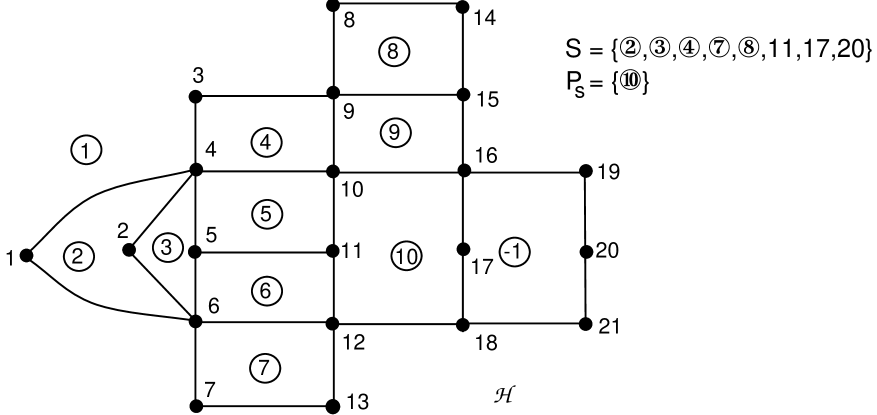
Figure 1: This is an example of a graph ${\cal H}$, a vf-set $S$, and ${\cal P}_{S}$, where a number in a circle is the index of the corresponding face.

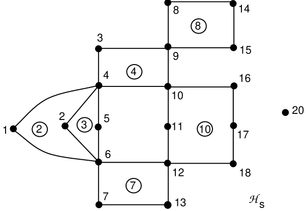
Figure 2: This is the graph ${\cal H}_{S}$ for the example of ${\cal H}$ and $S$ in Figure 1.

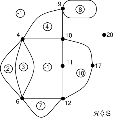
Figure 3: This is the graph ${\cal H}{\diamondsuit}S$ for the example of ${\cal H}$ and $S$ in Figure 1.

Let ${\cal P}_{S}$ be the set of the positive faces in ${\cal H}$ whose boundaries each contain at least two distinct vertices in $S\cap{\cal V}({\cal H})$. Let ${\cal H}_{S}$ be the plane subgraph of ${\cal H}$ (1) whose vertices are those in $S\cap{\cal V}({\cal H})$ and the boundary vertices of the faces in $(S\cap{\cal F}({\cal H}))\cup{\cal P}_{S}$ and (2) whose edges are the boundary edges of the faces in $(S\cap{\cal F}({\cal H}))\cup{\cal P}_{S}$. Note that ${\cal H}_{S}$ inherits a plane embedding from ${\cal H}$.

Let $U_{3}$ be the set of vertices which are of degree at least three in ${\cal H}_{S}$; note that each vertex in $U_{3}$ appears on the boundaries of at least two faces in $(S\cap{\cal F}({\cal H}))\cup{\cal P}_{S}$. A compressible path $P$ in ${\cal H}_{S}$ is a maximal path, which may be a cycle, such that (1) every internal vertex of $P$ appears only once in it, and (2) no internal vertex of $P$ is in $S\cup U_{3}$. Note that by the choice of $U_{3}$, every internal vertex of a compressible path is of degree 2 in ${\cal H}_{S}$. We use this property to further simplify ${\cal H}_{S}$. Let ${\cal H}{\diamondsuit}S$ be the plane graph obtained from ${\cal H}_{S}$ by replacing each compressible path with an edge between its endpoints. This edge is embedded by the same curve in the plane as the path is. For technical consistency, if a compressible path forms a cycle and its endpoint is not in $S\cup U_{3}$, then we replace it with a self-loop for the vertex of the cycle with the smallest index.

Each vertex in ${\cal H}{\diamondsuit}S$ is given the same index as in ${\cal H}$. Note that the closure of the interior of each face of ${\cal H}{\diamondsuit}S$ is the union of those of several faces or just one in ${\cal H}$. Let $F$ be a face in ${\cal H}{\diamondsuit}S$ and $F^{\prime}$ be one in ${\cal H}$. Let $\sigma$ (respectively, $\sigma^{\prime}$) denote the closure of the interior of $F$ (respectively, $F^{\prime}$). If $\sigma=\sigma^{\prime}$, then $F$ and $F^{\prime}$ are regarded as the same face, and $F$ is assigned the same index in ${\cal H}{\diamondsuit}S$ as $F^{\prime}$ is in ${\cal H}$. For technical conciseness, these two faces are identified with each other. If $\sigma$ is the union of the closures of the interiors of two or more faces in ${\cal H}$, $F$ is not the same as any face in ${\cal H}$ and is indexed by $-1$. This completes the definition of ${\cal H}{\diamondsuit}S$.

Lemma 3.4

1. Given ${\cal H}$ and $S$, we can compute ${\cal H}{\diamondsuit}S$ in $O(|{\cal H}|+|S|)$ time.

2. Let $S^{\prime}$ be a vf-set of ${\cal H}{\diamondsuit}S$. If $S^{\prime}\subseteq S$, then ${\cal H}{\diamondsuit}S^{\prime}=({\cal H}{\diamondsuit}S){\diamondsuit}S^{\prime}$.

3. If ${\cal H}$ simplifies ${\cal G}$ over a vf-set $S^{*}$ with $S\subseteq S^{*}$, then $|{\cal H}{\diamondsuit}S|=O(|S|)$.

Proof. Statements 1 and 2 are straightforward. To prove Statement 3, it suffices to prove $|{\cal G}{\diamondsuit}S|=O(|S|)$ since by Statement 2, ${\cal H}{\diamondsuit}S={\cal G}{\diamondsuit}S$.

To bound the number of vertices in ${\cal G}{\diamondsuit}S$, let ${\cal P}_{S}$ and $U_{3}$ be as specified in the definition of ${\cal G}{\diamondsuit}S$. Let $U_{1}$ be the set of vertices $v$ in ${\cal G}{\diamondsuit}S$ such that $v$ appears on the boundary of exactly one face in $(S\cap{\cal F}({\cal G}))\cup{\cal P}_{S}$. Then, $(S\cap{\cal V}({\cal G}))\cup U_{3}\cup U_{1}$ consists of all the vertices in ${\cal G}{\diamondsuit}S$. Note that $|U_{1}|\leq|(S\cap{\cal F}({\cal G}))\cup{\cal P}_{S}|$. Also, by Lemma 3.2(3), $|U_{3}|=O(|(S\cap{\cal F}({\cal G}))\cup{\cal P}_{S}|)$. Consequently, since by Lemma 3.2(2) $|{\cal P}_{S}|=O(|(S\cap{\cal V}({\cal G}))|)$, $|(S\cap{\cal V}({\cal G}))\cup U_{3}\cup U_{1}|=O(|S|)$ as desired.

To bound the number of edges in ${\cal G}{\diamondsuit}S$, we first examine the multiple edges. Let $u$ and $v$ be adjacent vertices in ${\cal G}{\diamondsuit}S$. Let $X_{u,v}$ be the set of faces in $(S\cap{\cal F}({\cal G}))\cup{\cal P}_{S}$ whose boundaries contain both $u$ and $v$. Then, $|X_{u,v}|\geq 1$. By Lemma 3.2(1), $|X_{u,v}|\leq 2$. If $X_{u,v}=\{F\}$, then the two boundary paths of $F$ between $u$ and $v$ may degenerate into at most two multiple edges between $u$ and $v$ in ${\cal G}{\diamondsuit}S$. If $X_{u,v}=\{F_{1},F_{2}\}$, then by the triconnectivity of ${\cal G}$, $F_{1}$ and $F_{2}$ share exactly one common boundary edge $e$, which is also an edge in ${\cal G}{\diamondsuit}S$. Let $C_{i}$ be the boundary of $F_{i}$ without $e$. $C_{1}$ and $C_{2}$ may degenerate into at most two multiple edges between $u$ and $v$ in ${\cal G}{\diamondsuit}S$. In summary, there are at most three multiple edges between two vertices in ${\cal G}{\diamondsuit}S$. Similarly, only the boundary of a face in $S\cap{\cal F}({\cal G})$ can degenerate into a self-loop in ${\cal G}{\diamondsuit}S$; so, ${\cal G}{\diamondsuit}S$ has only $O(|S|)$ self-loops. By Euler’s formula, ${\cal G}{\diamondsuit}S$ has $O(|S|)$ edges as desired.     

3.3 Algorithms for the ACF problem

Throughout this subsection, let ${\cal D}_{1},\ldots,{\cal D}_{q}$ be the vf-families in ${\cal N}$. To solve the ACF problem recursively, we use simplification to reduce the number of ${\cal D}_{i}$ and the number of sets in each ${\cal D}_{i}$.

For brevity, we define several notations. For a vf-family ${\cal D}$ of ${\cal H}$, let ${\cal H}{\diamondsuit}{\cal D}={\cal H}{\diamondsuit}(\cup_{S\in{\cal D}}S)$. For a vf-sequence ${\cal N}^{\prime}$: ${\cal D}^{\prime}_{1},\ldots,{\cal D}^{\prime}_{p}$ of ${\cal H}$, let ${\cal H}{\diamondsuit}{\cal N}^{\prime}={\cal H}{\diamondsuit}({\cal D}^{\prime}_{1}\cup\cdots\cup{\cal D}^{\prime}_{p})$. For a vf-set $S^{*}$ of ${\cal H}$ and a vf-family ${\cal D}$ of ${\cal H}$, we say ${\cal D}\leq S^{*}$ if $S\subseteq S^{*}$ for all $S\in{\cal D}$. For a vf-set $S^{*}$ of ${\cal H}$, we say ${\cal N}\leq S^{*}$ if ${\cal D}_{i}\leq S^{*}$ for all ${\cal D}_{i}$, $1\leq i\leq q$.

Lemmas 3.5 and 3.6 below reduce to $1$ the number of ${\cal D}_{i}$ in ${\cal N}$ in the ACF problem.

Lemma 3.5

Assume $q\geq 2$. Let ${\cal N}_{\ell}={\cal D}_{1},\ldots,{\cal D}_{\lceil q/2\rceil}$ and ${\cal N}_{r}={\cal D}_{\lceil q/2\rceil+1},\ldots,{\cal D}_{q}$. Let ${\cal H}_{\ell}={\cal H}{\diamondsuit}{\cal N}_{\ell}$ and ${\cal H}_{r}={\cal H}{\diamondsuit}{\cal N}_{r}$.

1. Given ${\cal H}$ and ${\cal N}$, we can compute ${\cal H}_{\ell}$ and ${\cal H}_{r}$ in $O(|{\cal H}|+|{\cal N}|)$ total time.

2. For $1\leq i\leq\lceil q/2\rceil$, ${\cal H}{\diamondsuit}{\cal D}_{i}={\cal H}_{\ell}{\diamondsuit}{\cal D}_{i}$. Similarly, for $\lceil q/2\rceil+1\leq i\leq q$, ${\cal H}{\diamondsuit}{\cal D}_{i}={\cal H}_{r}{\diamondsuit}{\cal D}_{i}$.

3. If ${\cal H}$ simplifies ${\cal G}$ over a vf-set $S^{*}$ with ${\cal N}\leq S^{*}$, then $|{\cal H}_{\ell}|=O(|{\cal N}_{\ell}|)$ and $|{\cal H}_{r}|=O(|{\cal N}_{r}|)$.

Proof. The three statements follow from those of Lemma 3.4, respectively.     

Lemma 3.6

Assume $q\geq 1$. Let ${\cal H}_{i}={\cal H}{\diamondsuit}{\cal D}_{i}$.

1. ${\rm ACF}({\cal H},{\cal D}_{i})={\rm ACF}({\cal H}_{i},{\cal D}_{i})$.

2. If ${\cal H}$ simplifies ${\cal G}$ over a vf-set $S^{*}$ with ${\cal N}\leq S^{*}$, then $|{\cal H}_{i}|=O(|{\cal D}_{i}|)$.

3. If ${\cal H}$ simplifies ${\cal G}$ over a vf-set $S^{*}$ with ${\cal N}\leq S^{*}$, then given ${\cal H}$ and ${\cal N}$, we can compute all ${\cal H}_{i}$ in $O(|{\cal H}|+|{\cal N}|\log(q+1))$ total time.

Proof. We prove the statements separately as follows.

Statement 1. The proof is straightforward. Note that a positive face in ${\cal H}_{i}$ is also a positive face in ${\cal H}$ and that a negative face in ${\cal H}_{i}$ combines one or more faces not in ${\rm ACF}({\cal H},{\cal D}_{i})$.

Statement 2. The proof follows from Lemma 3.4(3).

Statement 3. The graphs ${\cal H}_{i}$ can be computed by applying Lemma 3.5 recursively with $O(\log(q+1))$ iterations. By Lemma 3.5(1), the first iteration takes $O(|{\cal H}|+|{\cal N}|)$ time. By Lemmas 3.5(3) and 3.5(1), each subsequent iteration takes $O(|{\cal N}|)$ time. By Lemma 3.4(2), the constant coefficient in the $O(|{\cal N}|)$ term does not accumulate over recursions.     

Lemma 3.7 below solves the ACF problem with only one ${\cal D}_{i}$ in ${\cal N}$.

Lemma 3.7

Let ${\cal D}=\{S_{1},\ldots,S_{d}\}$ be a vf-family of ${\cal H}$ where $d\geq 1$. Let ${\cal D}^{\prime}_{\ell}=\{S_{1},\ldots,S_{\lceil d/2\rceil}\}$ and ${\cal D}^{\prime}_{r}=\{S_{\lceil d/2\rceil+1},\ldots,S_{d}\}$. Let ${\cal H}_{\ell}={\cal H}{\diamondsuit}{\cal D}^{\prime}_{\ell}$; ${\cal H}_{r}={\cal H}{\diamondsuit}{\cal D}^{\prime}_{r}$; and ${\cal D}^{\prime\prime}=\{{\rm ACF}({\cal H}_{\ell},{\cal D}^{\prime}_{\ell}),{\rm ACF}({\cal H}_{r},{\cal D}^{\prime}_{r})\}$.

1. ${\rm ACF}({\cal H},{\cal D})={\rm ACF}({\cal H},{\cal D}^{\prime\prime})$.

2. If ${\cal H}$ simplifies ${\cal G}$ over a vf-set $S^{*}$ with ${\cal D}\leq S^{*}$, then given ${\cal H}$ and ${\cal D}$, ${\rm ACF}({\cal H},{\cal D})$ can be computed in $O(|{\cal H}|+|{\cal D}|\log(d+1))$ time.

Proof. The statements are proved separately as follows.

Statement 1. Note that ${\rm ACF}({\cal H},{\cal D})={\rm ACF}({\cal H},\{{\rm ACF}({\cal H},{\cal D}^{\prime}_{\ell}),{\rm ACF}({\cal H},{\cal D}^{\prime}_{r})\})$ by a straightforward case analysis. Then, as Lemma 3.6(1), ${\rm ACF}({\cal H},{\cal D}^{\prime}_{\ell})={\rm ACF}({\cal H}_{\ell},{\cal D}^{\prime}_{\ell})$ and ${\rm ACF}({\cal H},{\cal D}^{\prime}_{r})={\rm ACF}({\cal H}_{r},{\cal D}^{\prime}_{r})$.

Statement 2. We compute ${\rm ACF}({\cal H},{\cal D})$ recursively via Statement 1. If $d=1$, then ${\rm ACF}({\cal H},{\cal D})=S_{1}$. If $d=2$, then ${\rm ACF}({\cal H},{\cal D})$ can be computed in $O(|{\cal H}|)$ time in a straightforward manner. For $d>2$, there are three stages:

1. Compute ${\cal H}_{\ell}$ and ${\cal H}_{r}$ in $O(|{\cal H}|+|D|)$ time in a straightforward manner.

2. Recursively compute ${\rm ACF}({\cal H}_{\ell},{\cal D}^{\prime}_{\ell})$ and ${\rm ACF}({\cal H}_{r},{\cal D}^{\prime}_{r})$.

3. Compute ${\rm ACF}({\cal H},{\cal D}^{\prime\prime})$ in $O(|{\cal H}|)$ time in a straightforward manner, which is ${\rm ACF}({\cal H},{\cal D})$ by Statement 1.

This recursive computation has $\log d+O(1)$ iterations. The recursion at the top level takes $O(|{\cal H}|+|{\cal D}|)$ time. Every subsequent level takes $O(|{\cal D}|)$ time since by Lemma 3.4(3) $O(|{\cal H}_{\ell}|)=O(|{\cal D}^{\prime}_{\ell}|)$ and $O(|{\cal H}_{r}|)=O(|{\cal D}^{\prime}_{r}|)$. Note that by Lemma 3.4(2), the constant coefficient in the $O(|{\cal D}|)$ term does not accumulate over recursions.     

The next theorem is the main result of this section.

Theorem 3.8

1. Let $d$ be the maximum number of vf-sets in any ${\cal D}_{i}$ in ${\cal N}$. If ${\cal H}$ simplifies ${\cal G}$ over a vf-set $S^{*}$ with ${\cal N}\leq S^{*}$, then the ACF problem can be solved in $O(|{\cal H}|+|{\cal N}|\log(d+q))$ time.

2. Let $d$ be the maximum number of vertex sets in any ${\cal C}_{i}$ in ${\cal M}$. Case M3 of the CFE problem can be solved in $O(|{\cal G}|+|{\cal M}|\log(d+q))$ time.

Proof. Statement 1 follows from Lemmas 3.6 and 3.7. Statement 2 follows from Observation 3.1, Statement 1, and the fact that ${\cal G}$ has a unique combinatorial embedding computable in linear time [21, 30].     

In §6.4, the algorithm for Case M2 of the CFE problem calls Theorem 3.8(2) to solve subproblems in which some $S\in{\cal C}_{i}$ may consist of a single edge $\{u,v\}$. For such subproblems, we replace $S$ by $\{u\}$ and $\{v\}$ and then apply Theorem 3.8(2).

4 Reducing Theorem 2.2 to Case M1 where ${\cal G}$ is connected.

Let ${\cal G}_{1},\ldots,{\cal G}_{k}$ be the connected components of ${\cal G}$. Let ${\cal C}_{1},\ldots,{\cal C}_{q}$ be the families in ${\cal M}$. A family ${\cal C}_{h}$ in ${\cal M}$ is global if for every $i\in\{1,\ldots,k\}$, ${\cal C}_{h}$ is not ${\cal G}_{i}$-local. Let $H$ be an edge-labeled graph defined as follows. The vertices of $H$ are $1,\ldots,k$. For each global ${\cal C}_{h}$, $H$ contains a cycle $C$ possibly of length 2 where (1) the vertices of $C$ are those $i\in\{1,\ldots,k\}$ such that some set in ${\cal C}_{h}$ is ${\cal G}_{i}$-local and (2) the edges of $C$ are all labeled $h$. See Figures 4(1) through 4(3) for an example of ${\cal G}$, ${\cal M}$ and $H$.

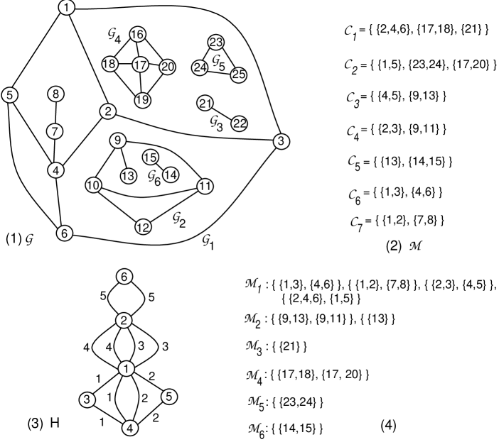
Figure 4: (1) This is a simple disconnected graph ${\cal G}$ with six connected components ${\cal G}_{1}$ through ${\cal G}_{6}$ where ${\cal V}({\cal G}_{1})=\{1,\ldots,8\}$, ${\cal V}({\cal G}_{2})=\{9,\ldots,13\}$, ${\cal V}({\cal G}_{3})=\{21,22\}$, ${\cal V}({\cal G}_{4})=\{16,\ldots,20\}$, ${\cal V}({\cal G}_{5})=\{23,\ldots,25\}$ and ${\cal V}({\cal G}_{6})=\{14,15\}$. (2) This is a sequence ${\cal M}$ of families of vertex subsets of ${\cal G}$ where ${\cal C}_{6}$ and ${\cal C}_{7}$ are ${\cal G}_{1}$-local but the rest families are global. (3) This is the graph $H$ constructed from ${\cal G}$ and ${\cal M}$. (4) These are the sequences constructed for ${\cal G}_{1}$ through ${\cal G}_{6}$, respectively.

Observation 4.1

Let $H_{1},\ldots,H_{\ell}$ be the connected components of $H$. For each $H_{j}$, let ${\cal G}^{\prime}_{j}$ be the subgraph of ${\cal G}$ formed by all ${\cal G}_{i}$ with $i\in{\cal V}(H_{j})$. Let ${\cal M}^{\prime}_{j}$ be the sequence of all ${\cal G}^{\prime}_{j}$-local families in ${\cal M}$. Then, ${\cal G}$ satisfies ${\cal M}$ if and only if every ${\cal G}^{\prime}_{j}$ satisfies ${\cal M}^{\prime}_{j}$.

By Observation 4.1, we may assume that $H$ is connected. Let $B_{1},\ldots,B_{p}$ be the blocks of $H$. Then, for each global ${\cal C}_{h}$, exactly one $B_{j}$ contains all the edges labeled $h$. For every $B_{j}$, let ${{\cal U}}_{j}=\cup_{h}{\cal C}_{h}$ where $h$ rangers over all labels on the edges of $B_{j}$. For each ${\cal G}_{i}$, let ${\cal M}_{i}$ be the sequence consisting of the ${\cal G}_{i}$-local families in ${\cal M}$ as well as the families ${{\cal U}}_{j,i}=\{U\in{{\cal U}}_{j}~{}|~{}U$ is ${\cal G}_{i}$-local$\}$ for all $B_{j}$ with $i\in{\cal V}(B_{j})$. See Figure 4(4) for an example of ${\cal M}_{1},\ldots,{\cal M}_{6}$ constructed from ${\cal G}$, ${\cal M}$ and $H$ in Figures 4(1) through 4(3).

Lemma 4.2

${\cal G}$ satisfies ${\cal M}$ if and only if every ${\cal G}_{i}$ satisfies ${\cal M}_{i}$.

Proof. The two directions are proved as follows.

$(\Longrightarrow)$ Let ${\Phi}$ be an embedding of ${\cal G}$ satisfying ${\cal M}$. Let ${\Phi}_{i}$ be the restriction of ${\Phi}$ to ${\cal G}_{i}$. For each ${\cal G}_{i}$, our goal is to prove that ${\Phi}_{i}$ satisfies ${\cal M}_{i}$. First, ${\Phi}_{i}$ satisfies each ${\cal G}_{i}$-local family in ${\cal M}$. Let $B_{j}$ be a block of $H$ with $i\in B_{j}$. We next prove that ${\Phi}_{i}$ satisfies ${{\cal U}}_{j,i}$. Let $i,i_{1},\ldots,i_{\ell}$ be the vertices of $B_{j}$. We claim that ${\cal G}$ has no cycle $C$ such that at least one but not all of ${\cal G}_{i}$, ${\cal G}_{i_{1}},\ldots,{\cal G}_{i_{\ell}}$ are inside $C$ in ${\Phi}$. To prove by contradiction, assume that such $C$ exists. Then, some ${\cal G}_{x}$ with $1\leq x\leq k$ contains $C$. However, by the construction of $H$, no connected component of $H-\{x\}$ contains all of $i$, $i_{1},\ldots,i_{\ell}$, contradicting the fact that $B_{j}$ is a block of $H$. Thus, the claim holds. Therefore, the boundary of some face $F$ in ${\Phi}$ intersects each of ${\cal G}_{i},{\cal G}_{i_{1}},\ldots,{\cal G}_{i_{\ell}}$. Since $F$ must be unique, the boundary of $F$ intersects every set in ${\cal C}_{h}$ for every ${\cal C}_{h}$ in ${\cal M}$ such that the sets in ${\cal C}_{h}$ fall into two or more of ${\cal G}_{i}$, ${\cal G}_{i_{1}}$, $\ldots$, ${\cal G}_{i_{\ell}}$. Hence, the boundary of $F$ intersects every set in ${{\cal U}}_{j}$. Consequently, ${\Phi}_{i}$ satisfies ${{\cal U}}_{j,i}$.

$(\Longleftarrow)$ Let ${\Phi}_{i}$ be an embedding of ${\cal G}_{i}$ satisfying ${\cal M}_{i}$. We construct an embedding of ${\cal G}$ satisfying ${\cal M}$ as follows. First, consider a block $B_{j}$ of $H$. Let $i_{1},\ldots,i_{\ell}$ be the vertices of $B_{j}$. Let ${\cal G}^{\prime}_{j}$ be the subgraph of ${\cal G}$ formed by ${\cal G}_{i_{1}}$, …, ${\cal G}_{i_{\ell}}$. Let ${\cal M}^{\prime}_{j}$ be the sequence consisting of ${{\cal U}}_{j}$ and the ${\cal G}_{i_{x}}$-local families in ${\cal M}$ for $x=1,\ldots,\ell$. We can assume that the boundary of the exterior face of ${\Phi}_{i_{x}}$ intersects every set in ${{\cal U}}_{j,i_{x}}$. By identifying the exterior faces of ${\Phi}_{i_{1}}$, …, ${\Phi}_{i_{\ell}}$, we can combine the embeddings into an embedding ${\Phi}^{\prime}_{j}$ of ${\cal G}^{\prime}_{j}$ satisfying ${\cal M}^{\prime}_{j}$. Next, we utilize $T=\Psi(H)$ to combine ${\Phi}^{\prime}_{1}$, …, ${\Phi}^{\prime}_{p}$ into a single embedding of ${\cal G}$. First, root $T$ at a block of $H$. For a leaf $B_{j_{1}}$ in $T$, let ${\cal G}_{i}$ and $B_{j_{2}}$ be the parent and grandparent of $B_{j_{1}}$ in $T$, respectively. Let ${{\cal L}}_{i,1}$ (respectively, ${{\cal L}}_{i,2}$) be the restriction of ${\Phi}^{\prime}_{j_{1}}$ (respectively, ${\Phi}^{\prime}_{j_{2}}$) to ${\cal G}_{i}$. Note that ${\Phi}_{i}$, ${{\cal L}}_{i,1}$, and ${{\cal L}}_{i,2}$ are topologically equivalent up to the choice of their exterior face. Thus, ${\Phi}^{\prime}_{j_{1}}$ (respectively, ${\Phi}^{\prime}_{j_{2}}$) can be obtained as follows: For every vertex $i^{\prime}\not=i$ of $B_{j_{1}}$ (respectively, $B_{j_{2}}$), put a suitable embedding ${{\cal L}}_{i^{\prime}}$ of ${\cal G}_{i^{\prime}}$ that is topologically equivalent to ${\Phi}_{i^{\prime}}$  into a suitable face $F_{i^{\prime}}$ of ${\Phi}_{i}$. This gives an embedding of those ${\cal G}_{x}\in\{{\cal G}_{1},\ldots,{\cal G}_{k}\}$ with $x\in{\cal V}(B_{j_{1}})\cup{\cal V}(B_{j_{2}})$. We replace ${\Phi}^{\prime}_{j_{2}}$ with this embedding, replace $B_{j_{2}}$ with the union of $B_{j_{1}}$ and $B_{j_{2}}$, and delete $B_{j_{1}}$ from $T$. Afterwards, if ${\cal G}_{i}$ becomes a leaf of $T$, then we further delete it from $T$. We repeat this process until $T$ is a single vertex, at which time we obtain an embedding of ${\cal G}$ satisfying ${\cal M}$.     

Theorem 4.3

Theorem 2.2 holds if it holds for Case M1.

Proof. The proof follows from Lemma 4.2 and the fact that $H$ and the sequences ${\cal M}_{i}$ above can be constructed from ${\cal G}$ and ${\cal M}$ in $O(I)$ time.     

5 Reducing Case M1 to Case M2 where ${\cal G}$ is biconnected.

This section assumes Case M1 where ${\cal G}$ is connected. We also assume that ${\cal G}$ has at least two vertices; otherwise, the problem is trivial.

Section 5.1 shows how to eliminate one cut vertex from ${\cal G}$; iterating this elimination until ${\cal G}$ has no cut vertex gives us a reduction from Case M1 to Case M2. However, this reduction is not efficient. Section 5.2 describes a more efficient reduction based on a direct elimination of all cut vertices from ${\cal G}$. Throughout the rest of this section, let ${\cal C}_{1},\ldots,{\cal C}_{q}$ be the families in ${\cal M}$.

5.1 Eliminating one cut vertex

Let $w$ be a cut vertex of ${\cal G}$. Let $W_{1}$, …, $W_{k}$ be the vertex sets of the connected components of ${\cal G}-\{w\}$. Let ${\cal G}_{i}$ be the subgraph of ${\cal G}$ induced by $\{w\}\cup W_{i}$. ${\cal G}_{1},\ldots,{\cal G}_{k}$ are called the augmented components induced by $w$. For each ${\cal C}_{h}$ in ${\cal M}$, let $U_{h,1}$, …, $U_{h,t_{h}}$ be the sets in ${\cal C}_{h}$ containing $w$; possibly $t_{h}=0$. ${\cal C}_{h}$ is $w$-global if for all $i\in\{1,\ldots,k\}$, ${\cal C}_{h}-\{U_{h,1},\ldots,U_{h,t_{h}}\}$ is not ${\cal G}_{i}$-local; otherwise, ${\cal C}_{h}$ is $w$-local.

Observation 5.1

1. Assume that ${\cal C}_{h}-\{U_{h,1},\ldots,U_{h,t_{h}}\}$ is ${\cal G}_{i}$-local for some ${\cal G}_{i}$. Then, ${\cal G}$ satisfies ${\cal M}$ if and only if ${\cal G}$ satisfies ${\cal M}$ with ${\cal C}_{h}$ replaced by $({\cal C}_{h}-\{U_{h,1},\ldots,U_{h,t_{h}}\})$ ${\cup}$ $\{U_{h,1}{\cap}{\cal V}({\cal G}_{i})$,…,$U_{h,t_{h}}{\cap}{\cal V}({\cal G}_{i})\}$.

2. Assume that ${\cal C}_{h}$ is $w$-global. Then, ${\cal G}$ satisfies ${\cal M}$ if and only if ${\cal G}$ satisfies ${\cal M}$ with ${\cal C}_{h}$ replaced by ${\cal C}_{h}-\{U_{h,1},\ldots,U_{h,t_{h}}\}$.

By Observation 5.1, we may assume that (1) each set in a $w$-global family in ${\cal M}$ does not contain $w$ and (2) each set in a family in ${\cal M}$ is ${\cal G}_{i}$-local for some ${\cal G}_{i}$. Let $H$ be an edge-labeled graph constructed as follows. The vertices of $H$ are $1,\ldots,k$. For each $w$-global family ${\cal C}_{h}$, $H$ has a cycle $C$ possibly of length 2 where (1) the vertices of $C$ are those $i\in\{1,\ldots,k\}$ such that at least one set in ${\cal C}_{h}$ is ${\cal G}_{i}$-local and (2) the edges of $C$ are all labeled $h$. See Figures 5(1) through 5(3) for an example of ${\cal G}$, ${\cal M}$ and $H$.

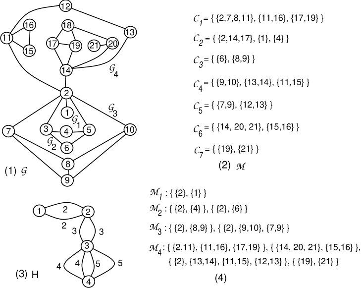
Figure 5: (1) This is a simple connected graph ${\cal G}$ with a cut vertex 2. It induces four augmented components ${\cal G}_{1}$ through ${\cal G}_{4}$ with ${\cal V}({\cal G}_{1})=\{1,2\}$, ${\cal V}({\cal G}_{2})=\{2,\ldots,6\}$, ${\cal V}({\cal G}_{3})=\{2,7,\ldots,10\}$ and ${\cal V}({\cal G}_{4})=\{2,11,\ldots,21\}$. (2) This is a sequence ${\cal M}$ of families of vertex subsets of ${\cal G}$ where only ${\cal C}_{2}$ through ${\cal C}_{5}$ are 2-global. (3) This is the graph $H$ constructed from ${\cal G}$ and ${\cal M}$. (4) These are the sequences constructed for ${\cal G}_{1}$ through ${\cal G}_{4}$, respectively.

Note that Observation 4.1 still holds for this $H$ and the augmented components ${\cal G}_{1},\ldots,{\cal G}_{k}$. Thus, we may assume that $H$ is connected. Let $B_{1}$, $\ldots$, $B_{p}$ be the blocks of $H$. Clearly, for each $w$-global family ${\cal C}_{h}\in{\cal M}$, exactly one block of $H$ contains all the edges labeled $h$. For each $B_{j}$, let ${{\cal U}}_{j}=\cup_{h}{\cal C}_{h}\cup\{\{w\}\}$ where $h$ ranges over all labels on the edges of $B_{j}$. For each ${\cal G}_{i}$, let ${\cal M}_{i}$ be the sequence consisting of the ${\cal G}_{i}$-local families in ${\cal M}$ as well as the families ${{\cal U}}_{j,i}=\{U\in{{\cal U}}_{j}~{}|~{}U$ is ${\cal G}_{i}$-local} for all $B_{j}$ with $i\in{\cal V}(B_{j})$. See Figure 5(4) for an example of ${\cal M}_{1},\ldots,{\cal M}_{4}$ constructed from ${\cal G}$, ${\cal M}$ and $H$ in Figures 5(1) through 5(3).

Lemma 5.2

${\cal G}$ satisfies ${\cal M}$ if and only if every ${\cal G}_{i}$ satisfies ${\cal M}_{i}$.

Proof. The two directions are proved as follows.

$(\Longrightarrow)$ The proof is the same as that of Lemma 4.2 except that the claim therein now implies that the boundary of some face $F$ in ${\Phi}$ intersects each of ${\cal G}_{i}-\{w\},{\cal G}_{i_{1}}-\{w\},\ldots,{\cal G}_{i_{\ell}}-\{w\}$.

$(\Longleftarrow)$ The proof is the same as that of Lemma 4.2 except that ${\Phi}^{\prime}_{j_{1}}$ (respectively, ${\Phi}^{\prime}_{j_{2}}$) now can be obtained as follows: For each vertex $i^{\prime}\not=i$ of $B_{j_{1}}$ (respectively, $B_{j_{2}}$), put a suitable embedding ${{\cal L}}_{i^{\prime}}$ of ${\cal G}_{i^{\prime}}$ that is topologically equivalent to $\Phi_{i^{\prime}}$ into a suitable face $F_{i^{\prime}}$ of ${\Phi}_{i}$, and then identify the two occurrences of $w$.     

5.2 Eliminating all cut vertices

Let $T=\Psi({\cal G})$. A block vertex of $T$ is a vertex of $T$ that is a block of ${\cal G}$. Root $T$ at a block vertex and perform a post-order traversal of $T$. For each vertex $\gamma$ of $T$, let ${\rm post}(\gamma)$ be the post-order number of $\gamma$ in the post-order traversal of $T$.

Let $W=\{w_{1},\ldots,w_{\ell}\}$ be the set of cut vertices of ${\cal G}$ where ${\rm post}(w_{1})<\cdots<{\rm post}(w_{\ell})$. For each $v\in{\cal V}({\cal G})-W$, let ${\rm post}(v)={\rm post}(B)$, where $B$ is the unique block of ${\cal G}$ with $v\in{\cal V}(B)$. We may assume ${\cal V}({\cal G})=\{1,\ldots,n\}$. For each $v\in{\cal V}({\cal G})$, the rank of $v$, denoted by ${\rm rank}(v)$, is $({\rm post}(v),v)$. The rank of a vertex $u$ is lower than that of another vertex $v$ if (1) ${\rm post}(u)<{\rm post}(v)$ or (2) ${\rm post}(u)={\rm post}(v)$ and $u<v$. For each $w_{i}\in W$, let $B_{i,1}$, …, $B_{i,k_{i}}$ be the children of $w_{i}$ in $T$. Let $B_{i,0}$ be the parent of vertex $w_{i}$ in $T$.

Theorem 5.3

Theorem 2.2 holds for Case M1 if it holds for Case M2.

Proof. It suffices to construct a sequence ${\cal M}[B]$ for each block $B$ of ${\cal G}$, with a total size of $O(I)$ in $O(I\log I)$ total time over all the blocks of ${\cal G}$, such that ${\cal G}$ satisfies ${\cal M}$ if and only if every $B$ satisfies ${\cal M}[B]$. To construct ${\cal M}[B]$ based on Observation 5.1 and Lemma 5.2, we process $w_{1}$, …, $w_{\ell}$ one at a time. During the processing of $w_{i}$, we construct ${\cal M}[B_{i,j}]$ for all $j=1,\ldots,k_{i}$. Then, we delete $w_{i}$, $B_{i,1}$, …, $B_{i,k_{i}}$ from $T$. After processing $w_{\ell}$, we are left with the root $B_{\ell,0}$ for which we then construct ${\cal M}[B_{\ell,0}]$.

We use the following data structures. See Figure 6 for an example of some of the data structures before processing the first cut vertex of ${\cal G}$.

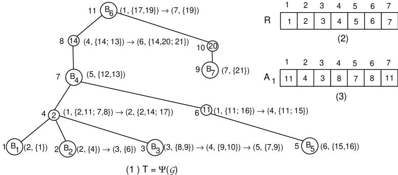
Figure 6: (1) This is $\Psi({\cal G})$ where ${\cal G}$ is the simple graph in Figure 5(1). Here, ${\cal V}(B_{1})=\{1,2\}$, ${\cal V}(B_{2})=\{2,\ldots,6\}$, ${\cal V}(B_{3})=\{2,7,\ldots,10\}$, ${\cal V}(B_{4})=\{2,11,\ldots,14\}$, ${\cal V}(B_{5})=\{11,15,16\}$, ${\cal V}(B_{6})=\{14,17,\ldots,20\}$, ${\cal V}(B_{7})=\{20,21\}$. The number to the left of each vertex $\gamma$ of $\Psi({\cal G})$ is ${\rm post}(\gamma)$, and the list to the right is $L(\gamma)$ before processing the first cut vertex of ${\cal G}$. For visibility, each set $U$ in a pair in $L(\gamma)$ with $U\cap W\neq\emptyset$ is divided into two parts via a semiclolon; the first part consists of vertices in $U\cap W$ in the increasing order of their post-order numbers. (2) These are the representatives in the union-find data structure before processing the first cut vertex of ${\cal G}$. (3) This is the array $A_{1}$ before processing the first cut vertex of ${\cal G}$.

1. During the construction, some families in ${\cal M}$ may be united, and we use a union-find data structure to maintain a collection of disjoint dynamic subsets of $\Delta=\{1,\ldots,q\}$. (Recall that $q$ is the number of families in ${\cal M}$.) Each subset of $\Delta$ in the data structure is identified by a representative member of the subset. For each $h\in\Delta$, let $R(h)$ be the representative of the subset containing $h$. Initially, each $h\in\Delta$ forms a singleton subset, and thus, $R(h)=h$.

2. Each set $U$ in a family in ${\cal M}$ is implemented as a pair $({{\cal W}}[U],{{\cal S}}[U])$, where ${{\cal W}}[U]$ is a linked list, and ${{\cal S}}[U]$ is a splay tree [28]. Initially, ${{\cal W}}[U]$ consists of the vertices in $U\cap W$ in the increasing order of their post-order numbers. ${{\cal S}}[U]$ is initialized by inserting the ranks of the vertices in $U-W$ into an empty splay tree. A splay tree supports the following operations in amortized logarithmic time per operation: (1) insert a rank and (2) delete the ranks in a given range.

3. A linked list $L[B]$, for each block $B$ of ${\cal G}$. Initially, each $L[B]$ consists of all pairs $(h,U)$ such that $h\in\Delta$, $U\in{\cal C}_{h}$, $U$ is $B$-local, and $U\cap W=\emptyset$.

4. A linked list $L[w_{i}]$, for each $w_{i}\in W$. Initially, each $L[w_{i}]$ consists of all pairs $(h,U)$ such that $h\in\Delta$, $U\in{\cal C}_{h}$, $w_{i}\in U$, and $i=\min\{j~{}|~{}w_{j}\in U\cap W\}$.

5. An array $A_{1}[1..q]$ of integers. Initially, for each $h\in\Delta$, $A_{1}[h]=\max_{\gamma}{\rm post}(\gamma)$ where $\gamma$ ranges over all vertices of $T$ such that $L[\gamma]$ contains a pair $(h,*)$ with $*$ = “don’t care”.

6. An array $A_{2}[1..q]$ of integers. Initially, for each $h\in\Delta$, $A_{2}[h]=0$.

7. An array $J[1..q]$ of linked lists of integers. Initially, for each $h\in\Delta$, $J[h]$ is empty.

8. A temporary array $Y[1..q]$ of integers.

We maintain the following invariants immediately before processing each $w_{i}$. In particular, we initialize the above data structures so that the invariants hold before $w_{1}$ is processed. It takes $O(I)$ total time to initialize the data structures except the splay trees.

1. For each vertex $\gamma$ of $T$ and each pair $(h,U)\in L[\gamma]$, (1) ${{\cal W}}[U]$ consists of the vertices in $U\cap\{w_{i},\ldots,w_{\ell}\}$ in the increasing order of their post-order numbers, (2) the rank of each vertex of $U-\{w_{i},\ldots,w_{\ell}\}$ is stored in ${{\cal S}}[U]$, and (3) for every $w_{j}\in U\cap\{w_{1},\ldots,w_{i-1}\}$, ${\rm post}(w_{j})$ and ${\rm rank}(w_{j})$ have been updated as ${\rm post}(B_{j,0})$ and $({\rm post}(B_{j,0}),w_{j})$, respectively.

2. For each block vertex $B$ of $T$ and each $(h,U)\in L[B]$, it holds that $h\in\Delta$, $U$ is $B$-local, and $U\cap\{w_{i},\ldots,w_{\ell}\}=\emptyset$.

3. For each $j\in\{i,\ldots,\ell\}$ and each $(h,U)\in L[w_{j}]$, it holds that $h\in\Delta$, $w_{j}\in U$, and $j=\min\{x~{}|~{}i\leq x\leq\ell$ and $w_{x}\in U\}$.

4. For each $h\in\Delta$ with $R(h)=h$, let ${\cal C}^{\prime}_{h}=\{U~{}|$ there is a vertex $\gamma$ of $T$ such that $L[\gamma]$ contains a pair $(h^{\prime},U)$ with $R(h^{\prime})=h\}$. Let ${\cal M}^{\prime}$ be the sequence of all families ${\cal C}^{\prime}_{h}$ such that $h\in\Delta$ and $R(h)=h$. Let ${\cal G}^{\prime}$ be the subgraph of ${\cal G}$ induced by $\cup_{B}{\cal V}(B)$, where $B$ ranges over all the block vertices of $T$. Then, ${\cal G}$ satisfies ${\cal M}$ if and only if (1) ${\cal G}^{\prime}$ satisfies ${\cal M}^{\prime}$ and (2) for each block $B$ of ${\cal G}$ that has been deleted from $T$, $B$ satisfies ${\cal M}[B]$.

5. For each $h\in\Delta$ with $R(h)=h$, $A_{1}[h]=\max_{\gamma}{\rm post}(\gamma)$ where $\gamma$ ranges over all vertices of $T$ such that $L[\gamma]$ contains a pair $(h^{\prime},*)$ with $R(h^{\prime})=h$.

6. For each $h\in\Delta$, $A_{2}[h]=0$ and $J[h]$ is empty.

We process $w_{i}$ in the following stages W1 through W4. See Figure 7 for an example of some of the data structures after processing the first cut vertex of ${\cal G}$.

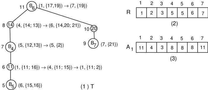
Figure 7: This is the data structure after processing the first cut vertex (i.e., the vertex 2) of the graph in Figure 7(1).

$\bullet$ Stage W1 checks whether each related family is $w_{i}$-global as follows.

1. Compute $X=\{h\in\Delta~{}|~{}R(h)=h$, and for some $j\in\{1,\ldots,k_{i}\}$, $L[B_{i,j}]$ contains a pair $(h^{\prime},*)$ with $R(h^{\prime})=h\}$. (Remark. For each $h\in\Delta-X$ with $R(h)=h$, the family ${\cal C}^{\prime}_{h}-\{U~{}|~{}w_{i}\in U\}$ is $Q_{i}$-local, where $Q_{i}$ is the augmented component of ${\cal G}^{\prime}$ induced by $w_{i}$ that is not among $B_{i,1}$, …, $B_{i,k_{i}}$. See the fourth invariant for ${\cal C}^{\prime}_{h}$ and ${\cal G}^{\prime}$.)

2. For each $h\in X$, set $Y[h]$ to be the number of integers $j\in\{1,\ldots,k_{i}\}$ such that $L[B_{i,j}]$ contains a pair $(h^{\prime},*)$ with $R(h^{\prime})=h$. (Remark. For $h\in X$, $Y[h]\geq 1$.)

3. For each $h\in X$, perform the following:

   1. If $Y[h]=1$ and $A_{1}[h]\leq{\rm post}(w_{i})$, then set $A_{2}[h]=j$ where $j$ is the unique integer in $\{1,\ldots,k_{i}\}$ such that $L[B_{i,j}]$ contains a pair $(h^{\prime},*)$ with $R(h^{\prime})=h$. (Remark. ${\cal C}^{\prime}_{h}-\{U~{}|~{}w_{i}\in U\}$ is $B_{i,j}$-local.)

   2. Otherwise set $A_{2}[h]=-1$. (Remark. ${\cal C}^{\prime}_{h}-\{U~{}|~{}w_{i}\in U\}$ is $w_{i}$-global.)

$\bullet$ Stage W2 modifies each $U$ with $w_{i}\in U$ in each $w_{i}$-local family based on Observation 5.1(1) as follows.

1. For each $(h,U)\in L[w_{i}]$ with $A_{2}[R(h)]\geq 1$, let $j=A_{2}[R(h)]$, delete all vertices outside ${\cal V}(B_{i,j})$ from $U$, and then insert $(h,U)$ to $L[B_{i,j}]$. Here, deleting all vertices outside ${\cal V}(B_{i,j})$ from $U$ is done as follows: Delete $w_{i}$ from ${{\cal W}}[U]$, delete all the ranks in the range $[-\infty..({\rm post}(B_{i,j}),0)]$ and all the ranks in the range $[({\rm post}(B_{i,j}),n+1)..\infty]$ from ${{\cal S}}[U]$, and insert $({\rm post}(B_{i,j}),w_{i})$ to ${{\cal S}}[U]$.

2. For each $(h,U)\in L[w_{i}]$ with $A_{2}[R(h)]=0$, perform the following:
   (Remark. ${\cal C}^{\prime}_{h}-\{U~{}|~{}w_{i}\in U\}$ is $Q_{i}$-local. See the remark in Step 1 of Stage W1 for $Q_{i}$.)

   1. Delete all vertices $v$ with ${\rm post}(v)<{\rm post}(w_{i})$ from $U$ as follows: Delete $w_{i}$ from ${{\cal W}}[U]$, delete all the ranks in the range $[-\infty..{\rm rank}(w_{i})]$ from ${{\cal S}}[U]$, and insert $({\rm post}(B_{i,0}),w_{i})$ to ${{\cal S}}[U]$.

   2. If ${{\cal W}}[U]=\emptyset$, i.e., $U$ has no cut vertex, then insert $(h,U)$ to $L[B_{i,0}]$ and set $A_{1}[R(h)]=\max\{{\rm post}(B_{i,0}),A_{1}[R(h)]\}$.

   3. If ${{\cal W}}[U]\not=\emptyset$, then find the first vertex $w_{j}$ in ${{\cal W}}[U]$, insert $(h,U)$ to $L[w_{j}]$, and set $A_{1}[R(h)]=\max\{{\rm post}(w_{j}),A_{1}[R(h)]\}$. (Remark. $j>i$.)

$\bullet$ Stage W3 modifies each $w_{i}$-global family based on Observation 5.1(2) as follows.

1. For each $h\in X$ with $A_{2}[h]=-1$, set $J[h]=\{j\in\{1,\ldots,k_{i}\}~{}|~{}L[B_{i,j}]$ contains a pair $(h^{\prime},*)$ with $R(h^{\prime})=h\}$.

2. For each $h\in X$ with $A_{2}[h]=-1$ and $A_{1}[h]>{\rm post}(w_{i})$, insert 0 to $J[h]$.

3. Set ${\rm post}(w_{i})={\rm post}(B_{i,0})$ and ${\rm rank}(w_{i})=({\rm post}(B_{i,0}),w_{i})$.

4. Construct an edge-labeled graph $H_{i}$ as follows. The vertices of $H_{i}$ are $0$, $1$, …, $k_{i}$. For each $h\in X$ with $A_{2}[h]=-1$, $H_{i}$ has a cycle possibly of length 2 whose vertices are the integers in $J[h]$ and whose edges are all labeled $h$.

5. For each block ${{\cal B}}$ of $H_{i}$, find the labels $h_{1},\ldots,h_{t}$ on the edges in ${{\cal B}}$ and unite those subsets in the union-find data structure that have $h_{1},\ldots,h_{t}$ as their representative, respectively; afterwards, for the representative $h_{r}$ of the resulting subset, further perform the following:

   1. Insert $(h_{r},\{w_{i}\})$ to all lists $L[B_{i,j}]$ such that $j\in{\cal V}({{\cal B}})$.

   2. If $0\in{\cal V}({{\cal B}})$, then set $A_{1}[h_{r}]=\max\{{\rm post}(B_{i,0})$, $A_{1}[h_{1}]$, …, $A_{1}[h_{t}]\}$.

$\bullet$ Stage W4 constructs the sequences ${\cal M}[B_{i,j}]$ for $1\leq j\leq k_{i}$ and updates the data structures as follows.

1. For each $j$ and each $(h,U)$ in $L[B_{i,j}]$, replace $(h,U)$ by $(R(h),U)$.

2. For each $j$, set ${\cal M}[B_{i,j}]$ to be the sequence of the families ${\cal C}^{\prime\prime}_{h}=\{U~{}|~{}(h,U)\in L[B_{i,j}]\}$, where $h$ ranges over those integers that are in a pair in $L[B_{i,j}]$.

3. Delete $w_{i}$ and its children from $T$.

4. For each $h\in X$, set $A_{2}[h]=0$ and $J[h]=\emptyset$.

By Observation 5.1 and Lemma 5.2, after the processing of $w_{i}$, the invariants hold for $i+1$.

After processing $w_{\ell}$, we construct ${\cal M}[B_{\ell,0}]$ as follows: Replace each pair $(h,U)$ in $L[B_{\ell,0}]$ by $(R(h),U)$, and then set ${\cal M}[B_{\ell,0}]$ to be the sequence of the families ${\cal C}^{\prime\prime}_{h}=\{U~{}|~{}(h,U)\in L[B_{\ell,0}]\}$, where $h$ ranges over those integers that are in a pair in $L[B_{\ell,0}]$.

By the invariants, Observation 5.1, and Lemma 5.2, ${\cal G}$ satisfies ${\cal M}$ if and only if every block $B$ of ${\cal G}$ satisfies ${\cal M}[B]$. As for the time complexity, we make the following observations:

1. When processing $w_{i}$, we create at most $n_{i}$ new sets all equal to $\{w_{i}\}$, where $n_{i}$ is the maximum number of blocks in a simple graph with $k_{i}+1$ vertices. Since $n_{i}=O(k_{i}+1)$ and $k_{i}+1$ does not exceed the degree of $w_{i}$ in ${\cal G}$, the total number of newly created sets is $O(|{\cal G}|)$.

2. If a set $U$ does not intersect $\{w_{i},\ldots,w_{\ell}\}$ immediately before the processing of $w_{i}$, then there is at most one $w_{j}\in\{w_{i},\ldots,w_{\ell}\}$ such that some vertices of $U$ are touched during the processing of $w_{j}$.

3. If $w_{i}$ is in $U$ immediately before the processing of $w_{i}$, then we either (1) touch at most $1+|\{v\in U~{}|~{}{\rm post}(v)\leq{\rm post}(w_{i})\}|$ vertices of $U$ during the processing of $w_{i}$, or (2) touch no vertex of $U$ during the processing of each $w_{j}\in\{w_{i+1},\ldots,w_{\ell}\}$.

There are at most $q$ unions and $O(I)$ finds, and at most $|{\cal G}|$ insertions into each splay tree. By the above observations, the total time spent on the union-find data structure is $O(I\log I)$, that on the splay trees is $O(I\log|{\cal G}|)$, and that on the remaining computation is $O(I)$, all within the desired time.     

6 Case M2 where ${\cal G}$ is biconnected.

This section assumes that ${\cal G}$ is biconnected. Let ${\cal C}_{1},\ldots,{\cal C}_{q}$ be the families in ${\cal M}$. For each $i\in\{1,\ldots,q\}$, let ${\cal C}_{i}=\{U_{i,1},\ldots,U_{i,r_{i}}\}$.

Theorem 6.1

Theorem 2.2 holds for Case M2.

To prove Theorem 6.1, we review a decomposition of ${\cal G}$ in §6.1, outline the basic ideas of our CFE algorithm in §6.2, detail the algorithm in §6.3, and analyze it in §6.4.

6.1 SPQR decompositions

A planar $st$-graph $G$ is a directed acyclic plane graph such that $G$ has exactly one source $s$ and exactly one sink $t$, and both vertices are on the exterior face. These two vertices are the poles of $G$. A split pair of $G$ is either a pair of adjacent vertices or a pair of vertices whose removal disconnects the graph obtained from $G$ by adding the edge $(s,t)$. A split component of a split pair $\{u,v\}$ is either an edge $(u,v)$ or a maximal subgraph $C$ of $G$ such that $C$ is a planar $uv$-graph and $\{u,v\}$ is not a split pair of $C$. A split pair $\{u,v\}$ of $G$ is maximal if there is no other split pair $\{u^{\prime},v^{\prime}\}$ in $G$ such that a split component of $\{u^{\prime},v^{\prime}\}$ contains both $u$ and $v$.

The decomposition tree $T$ of $G$ is a rooted ordered tree recursively defined in four cases as follows. The nodes of $T$ are of four types $S,P,Q$, and $R$. Each node $\mu$ of $T$ has an associated planar $st$-graph ${\rm ske}(\mu)$, called the skeleton of $\mu$. Also, $\mu$ is associated with an edge in the skeleton of the parent $\phi$ of $\mu$, called the virtual edge of $\mu$ in ${\rm ske}(\phi)$.

Case Q: $G$ is a single edge from $s$ to $t$. Then, $T$ is a Q-node whose skeleton is $G$.

Case S: $G$ is not biconnected. Let $c_{1},\ldots,c_{k-1}$ with $k\geq 2$ be the cut vertices of $G$. Since $G$ is a planar $st$-graph, each $c_{i}$ is in exactly two blocks $G_{i}$ and $G_{i+1}$ with $s\in G_{1}$ and $t\in G_{k}$. Then, $T$’s root is an S-node $\mu$, and ${\rm ske}(\mu)$ consists of the chain $e_{1},\ldots,e_{k}$, where the edge $e_{i}$ goes from $c_{i-1}$ to $c_{i}$, $c_{0}=s$, and $c_{k}=t$.

Case P: $\{s,t\}$ is a split pair of $G$ with $k$ split components where $k\geq 2$. Then, $T$’s root is a P-node $\mu$, and ${\rm ske}(\mu)$ consists of $k$ parallel edges $e_{1},\ldots,e_{k}$ from $s$ to $t$.

Case R: Otherwise. Let $\{s_{1},t_{1}\},\ldots,\{s_{k},t_{k}\}$ with $k\geq 1$ be the maximal split pairs of $G$. Let $G_{i}$ be the union of the split components of $\{s_{i},t_{i}\}$. Then, $T$’s root is an R-node $\mu$, and ${\rm ske}(\mu)$ is the simple graph obtained from $G$ by replacing each $G_{i}$ with an edge $e_{i}$ from $s_{i}$ to $t_{i}$. Note that adding the edge $(s,t)$ to ${\rm ske}(\mu)$ yields a simple triconnected graph.

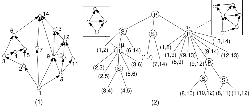
Figure 8: The tree in $($2$)$ is the decomposition tree of the graph in $($1$)$.

Figure 8 illustrates the decomposition tree of $G$ as well as the skeletons of $\mu$ and $\nu$. In the last three cases, $\mu$ has children $\chi_{1},\ldots,\chi_{k}$ in this order, such that each $\chi_{i}$ is the root of the decomposition tree of $G_{i}$. The virtual edge of $\chi_{i}$ is the edge $e_{i}$ in ${\rm ske}(\mu)$. $G_{i}$ is called the pertinent graph ${\rm pert}(\chi_{i})$ of $\chi_{i}$ as well as the expansion graph of $e_{i}$. Note that $G$ is the pertinent graph of $T$’s root. Also, no child of an S-node is an S-node, and no child of a P-node is a P-node.

The allocation nodes of a vertex $v$ of $G$ are the nodes of $T$ whose skeleton contains $v$; note that $v$ has at least one allocation node.

Lemma 6.2 (see [2])

1. $T$ has $O(|G|)$ nodes and can be constructed in $O(|G|)$ time. The total number of edges of the skeletons stored at the nodes of $T$ is $O(|G|)$.

2. The pertinent graphs of the children of $\mu$ can only share vertices of ${\rm ske}(\mu)$.

3. If $v$ is in ${\rm ske}(\mu)$, then $v$ is also in the pertinent graph of all ancestors of $\mu$.

4. If $v$ is a pole of ${\rm ske}(\mu)$, then $v$ is also in the skeleton of the parent of $\mu$. If $v$ is in ${\rm ske}(\mu)$ but is not a pole of ${\rm ske}(\mu)$, then $v$ is not in the skeleton of any ancestor of $\mu$.

5. The least common ancestor $\mu$ of the allocation nodes of $v$ itself is an allocation node of $v$, called the proper allocation node of $v$. Also, if $v\not\in\{s,t\}$, then $\mu$ is the only allocation node of $v$ such that $v$ is not a pole of ${\rm ske}(\mu)$.

6. If $v\neq s,t$, then the proper allocation node of $v$ is an R-node or S-node.

For each non-S-node $\mu$ in $T$, ${\rm pert}(\mu)$ is called a block of $G$ [2], which differs from that in §4 and §5. For a block $B={\rm pert}(\mu)$, let ${\rm node}(B)=\mu$. For an ancestor $\phi$ of ${\rm node}(B)$, the representative of $B$ in ${\rm ske}(\phi)$ is the edge in ${\rm ske}(\phi)$ whose expansion graph contains $B$.

Let $\mu$ be an R-node or P-node in $T$ with children $\chi_{1},\ldots,\chi_{b}$. For each $k\in\{1,\ldots,b\}$, let $e_{k}$ be the virtual edge of $\chi_{k}$ in ${\rm ske}(\mu)$. If $\chi_{k}$ is an S-node, ${\rm pert}(\chi_{k})$ is a chain consisting of two or more blocks. If $\chi_{k}$ is an R-node or P-node, ${\rm pert}(\chi_{k})$ is a single block. For each $k\in\{1,\ldots,b\}$, we say that the blocks in ${\rm pert}(\chi_{k})$ are on edge $e_{k}$. The minor blocks of ${\rm pert}(\mu)$ are the blocks on $e_{1}$, …, the blocks on $e_{b}$.

6.2 Basic ideas

An $st$-orientation of a planar graph is an orientation of its edges together with an embedding such that the resulting digraph is a planar $st$-graph.

Lemma 6.3 (see [1, 2])

If an $n$-vertex simple planar graph has an $st$-orientation, then every embedding, where $s$ and $t$ are on the exterior face, of this graph can be obtained from this orientation through a sequence of $O(n)$ following operations:

1. Flip an R-node’s skeleton around its poles.

2. Permute a P-node’s children (and consequently their skeletons with respect to their common poles).

Let $\{s,t\}$ be an edge of ${\cal G}$. Since ${\cal G}$ is a simple biconnected graph, we convert ${\cal G}$ to a planar $st$-graph in $O(n)$ time [12] for technical convenience. For the remainder of §6, let $T$ be the decomposition tree of ${\cal G}$.

The CFE algorithm processes the nodes of $T$ in a bottom-up manner. It first processes the leaf nodes of $T$. When processing a node $\mu$, for each ${\cal C}_{i}$ such that ${\rm pert}(\mu)$ is the smallest block that intersects every set in ${\cal C}_{i}$, the algorithm looks for an embedding of ${\rm pert}(\mu)$ that satisfies ${\cal C}_{i}$. If this is impossible, the algorithm outputs “no” and stops; otherwise, it continues on to process the next node of $T$. We note, in passing, that Theorem 3.8(2) is used when processing R-nodes.

Let $\mu$ be a node of $T$. $T_{\mu}$ denotes the subtree of $T$ rooted at $\mu$ and $0pt(\mu)$ denotes the distance from $T$’s root to $\mu$. We need the following definitions:

1. $U_{i,j}$ is contained in ${\rm pert}(\mu)$ if the vertices of $U_{i,j}$ are all in ${\rm pert}(\mu)$; $U_{i,j}$ is strictly contained in ${\rm pert}(\mu)$ if in addition, no pole of ${\rm pert}(\mu)$ is in $U_{i,j}$.

2. Let ${\rm done}(U_{i,j})$ be the deepest node $\mu$ in $T$ such that $U_{i,j}$ is strictly contained in ${\rm pert}(\mu)$, if such a node exists. If no such $\mu$ exists, then $U_{i,j}$ contains a pole of ${\cal G}$ and let ${\rm done}(U_{i,j})$ be $T$’s root.

3. A family ${\cal C}_{i}$ straddles ${\rm pert}(\mu)$ if at least one set in ${\cal C}_{i}$ is strictly contained in ${\rm pert}(\mu)$, and at least one set in ${\cal C}_{i}$ has no vertex in ${\rm pert}(\mu)$.

4. Let ${\rm done}({\cal C}_{i})$ be the deepest node $\mu$ in $T$ such that for every $U_{i,j}\in{\cal C}_{i}$, at least one vertex of $U_{i,j}$ is in ${\rm pert}(\mu)$.

5. Let ${\rm sub}(\mu)=\{U_{i,j}~{}|~{}{\rm done}(U_{i,j})=\mu\}$ and ${\rm fam}(\mu)=\{{\cal C}_{i}~{}|~{}{\rm done}({\cal C}_{i})=\mu\}$.

6. If $\mu$ is a P-node or R-node, let ${\rm xfam}(\mu)={\rm fam}(\mu)\cup(\cup_{\chi_{k}}{\rm fam}(\chi_{k}))$ and ${\rm xsub}(\mu)={\rm sub}(\mu)\cup(\cup_{\chi_{k}}{\rm sub}(\chi_{k}))$, where $\chi_{k}$ ranges over all S-children of $\mu$.

In a fixed embedding of a block $B$, the poles of $B$ divide the boundary of its exterior face into two paths ${\rm side}_{1}(B)$ and ${\rm side}_{2}(B)$, called the two sides of $B$. $U_{i,j}$ is two-sided for $B$ if both ${\rm side}_{1}(B)$ and ${\rm side}_{2}(B)$ intersect $U_{i,j}$. In particular, $U_{i,j}$ is two-sided for $B$ if it contains a pole of $B$. $U_{i,j}$ is side-1 (respectively, side-2) for $B$ if only ${\rm side}_{1}(B)$ (respectively, ${\rm side}_{2}(B)$) intersects $U_{i,j}$. Assume that $B$ is a minor block of ${\rm pert}(\mu)$ for some $\mu$. Let $e_{k}$ be the representative of $B$ in ${\rm ske}(\mu)$. In a fixed embedding of ${\rm ske}(\mu)$, $e_{k}$ separates two faces $F$ and $F^{\prime}$. When embedding ${\rm pert}(\mu)$, we can embed ${\rm side}_{1}(B)$ towards either $F$ or $F^{\prime}$, referred to as the two orientations of $B$ in ${\rm pert}(\mu)$.

A family ${\cal C}_{i}$ is side-0 (respectively, side-1 or side-2) exterior-forcing for $B$ if ${\rm done}({\cal C}_{i})$ is an ancestor of ${\rm node}(B)$ in $T$ and some $U_{i,j}\in{\cal C}_{i}$ strictly contained in $B$ is two-sided (respectively, side-1 or side-2) for $B$. For $p=0$, 1, 2, define

1. ${\rm ext}_{p}(B)=$ $\min\{0pt({\rm done}({\cal C}_{i}))~{}|~{}{\cal C}_{i}$, $1\leq i\leq q$, is side-$p$ exterior-forcing for $B\}$, if at least one family in ${\cal M}$ is side-$p$ exterior-forcing for $B$;

2. ${\rm ext}_{p}(B)=\infty$ otherwise.

Assume ${\rm ext}_{p}(B)\not=\infty$. Let $\mu={\rm node}(B),\phi_{1},\phi_{2},\ldots,\phi_{h}$ be the path in $T$ from $\mu$ to $\phi_{h}$, where $0pt(\phi_{h})={\rm ext}_{p}(B)$. For each $\ell\in\{1,\ldots,h-1\}$, the representative of $B$ in ${\rm ske}(\phi_{\ell})$ must be an exterior edge in any satisfying embedding of ${\rm ske}(\phi_{\ell})$. In addition, if $p=1$ or 2, ${\rm side}_{p}(B)$ must be embedded towards the exterior face of the embedding of ${\rm pert}(\phi_{\ell})$.

Since $(s,t)$ is an edge of ${\cal G}$, the root $\rho$ of $T$ is a P-node and has a child Q-node $\phi$ representing $(s,t)$. A subtle difference between $\rho$ and each non-root node of $T$ is that the two sides of ${\cal G}={\rm pert}(\rho)$ is actually on the same face. To eliminate this difference, we delete $\phi$ from $T$; afterwards, if $\rho$ has only one child, we further delete $\rho$ from $T$. From here onwards, $T$ denotes this modified tree.

6.3 The CFE algorithm

The CFE algorithm processes $T$ from bottom up. A ready node $\mu$ of $T$ is either (1) a leaf node or (2) a P-node or R-node such that the non-S-children of $\mu$ and the children of every S-child of $\mu$ all have been processed. The CFE algorithm processes the ready nodes of $T$ in an arbitrary order. An S-node is processed when its parent is processed. We detail how to process $\mu$ as follows.

For the case where $\mu$ is a leaf node of $T$, note that ${\rm pert}(\mu)$ is a single edge of ${\cal G}$. Since no $U_{i,j}$ is strictly contained in ${\rm pert}(\mu)$, ${\rm sub}(\mu)=\emptyset$. Also, each ${\cal C}_{i}\in{\rm fam}(\mu)$ is satisfied by every embedding of ${\cal G}$. Therefore, we simply set ${\rm ext}_{p}({\rm pert}(\mu))=\infty$ for $p=0,1,2$.

We next consider the case where $\mu$ is a non-leaf ready node. Before $\mu$ is processed, an embedding of every minor block of ${\rm pert}(\mu)$ is already fixed, except for a possible flip around its poles. Moreover, for each minor block $B$ of ${\rm pert}(\mu)$ and each $p\in\{0,1,2\}$, ${\rm ext}_{p}(B)$ is known. When processing $\mu$, the CFE algorithm checks whether some embedding ${\Phi}_{\mu}$ of ${\rm pert}(\mu)$ satisfies the following two conditions:

1. ${\Phi}_{\mu}$ satisfies every ${\cal C}_{i}$ in ${\rm xfam}(\mu)$.

2. For each ${\cal C}_{i}$ straddling ${\rm pert}(\mu)$ and each $U_{i,j}\in{\cal C}_{i}$ strictly contained in ${\rm pert}(\mu)$, at least one vertex of $U_{i,j}$ is embedded on the exterior face of ${\Phi}_{\mu}$. (Remark. This ensures the existence of an embedding of ${\rm pert}({\rm done}({\cal C}_{i}))$ satisfying ${\cal C}_{i}$ later.)

If no such ${\Phi}_{\mu}$ exists, then ${\cal G}$ cannot satisfy ${\cal M}$ and the CFE algorithm outputs “no” and stops. Otherwise, it finds such an ${\Phi}_{\mu}$ and fixes it except for a possible flip around its poles. It also computes ${\rm ext}_{p}({\rm pert}(\mu))$ for $p=0$, 1, 2.

To detail how to process $\mu$, we classify the sets $U_{i,j}$ that intersect ${\rm pert}(\mu)$ into four types and define a set ${\rm img}(U_{i,j},\mu)$ for each type as follows.

Type 1: $U_{i,j}$ contains at least one pole of ${\rm ske}(\mu)$. Then, ${\rm done}(U_{i,j})$ is an ancestor of $\mu$. Let ${\rm img}(U_{i,j},\mu)=\{v\in U_{i,j}~{}|~{}v$ is a vertex in ${\rm ske}(\mu)\}$.

Type 2: $U_{i,j}$ contains at least one vertex but no pole of ${\rm ske}(\mu)$. Then, ${\rm done}(U_{i,j})=\mu$. Let ${\rm img}(U_{i,j},\mu)$ as in the case of type 1.

Type 3: $U_{i,j}$ is strictly contained in ${\rm pert}(\chi)$ for some S-node child $\chi$ of $\mu$ and $U_{i,j}$ contains at least one vertex in ${\rm ske}(\chi)$. Then, ${\rm done}(U_{i,j})=\chi$. Let ${\rm img}(U_{i,j},\mu)$ consist of the virtual edge of $\chi$ in ${\rm ske}(\mu)$.

Type 4: $U_{i,j}$ is strictly contained in a minor block $B$ of ${\rm pert}(\mu)$. Then, ${\rm done}(U_{i,j})$ is ${\rm node}(B)$ or its descendent. Let ${\rm img}(U_{i,j},\mu)$ consist of the representative of $B$ in ${\rm ske}(\mu)$.

Each element of ${\rm img}(U_{i,j},\mu)$ is called an image of $U_{i,j}$ in ${\rm ske}(\mu)$. The remainder of §6.3 details how to process $\mu$.

6.3.1 Processing an S-child of $\mu$

When processing $\mu$, for each S-child $\chi$ of $\mu$, we need to find an embedding of ${\rm pert}(\chi)$ satisfying certain conditions. We call this process the S-procedure and describe it below.

Let $\chi$ be an S-child of $\mu$. Then, ${\rm ske}(\chi)$ is a path. Let $e_{1}$, …, $e_{b}$ be the edges in ${\rm ske}(\chi)$. For each $k\in\{1,\ldots,b\}$, let $B_{k}$ be the expansion graph of $e_{k}$. Before the S-procedure is called on $\chi$, the following requirements are met:

1. For each $k\in\{1,\ldots,b\}$, an embedding of $B_{k}$ has been fixed, except for a possible flip around its poles.

2. For some integers $k\in\{1,\ldots,b\}$ and $p\in\{1,2\}$, ${\rm side}_{p}(B_{k})$ is required to face either the left or the right side of ${\rm ske}(\chi)$.

Our only choice for embedding ${\rm pert}(\chi)$ is to flip $B_{1}$, …, $B_{b}$ around their poles. We need to check whether for some combination of flippings of $B_{1}$, …, $B_{b}$, (1) the resulting embedding satisfies every ${\cal C}_{i}\in{\rm fam}(\chi)$ and (2) the second requirement above is met.

The S-procedure consists of the following five stages:

$\bullet$ Stage S1 constructs an auxiliary graph $D=(V_{D},E_{D})$ with $V_{D}=\{k_{p}~{}|~{}1\leq k\leq b,~{}p=1,2\}$ as follows. For each ${\cal C}_{i}\in{\rm fam}(\chi)$, insert an arbitrary path $P_{i}$ into $D$ to connect all $k_{p}\in V_{D}$ such that for some type-4 $U_{i,j}\in{\cal C}_{i}$, (a) ${\rm img}(U_{i,j},\chi)=\{e_{k}\}$ and (b) $U_{i,j}$ is side-$p$ for $B_{k}$. To avoid confusion, we call the elements of $V_{D}$ points, and the connected components of $D$ clusters. Those points $k_{p}\in V_{D}$ such that ${\rm side}_{p}(B_{k})$ is required to face the left side of ${\rm ske}(\chi)$ are called $L$-points. R-points are defined similarly. Note that for each cluster $C$ of $D$, all ${\rm side}_{p}(B_{k})$ where $k_{p}$ ranges over all the points in $C$ must be embedded toward the same side of ${\rm ske}(\chi)$. Also, each type-3 $U_{i,j}$ in ${\cal C}_{i}$ contains a vertex in ${\rm ske}(\chi)$ which is on both sides of ${\rm ske}(\chi)$. For this reason, such sets were not considered when constructing $D$.

$\bullet$ Stage S2 checks whether there is a cluster of $D$ containing both an $L$-point and an R-point. If such a cluster exists, then S2 outputs “no” and stops. Suppose that no such cluster exists. If a cluster $C$ contains an $L$-point (respectively, $R$-point), we call $C$ an $L$-cluster (respectively, $R$-cluster).

$\bullet$ Stage S3 constructs another auxiliary graph $RD=(V_{RD},E_{RD})$ from $D$ as follows. The vertices of $RD$ are the clusters of $D$. For each $k\in\{1,\ldots,b\}$, there is an edge $\{C_{1},C_{2}\}$ in $RD$, where $C_{1}$ (respectively, $C_{2}$) is the cluster of $D$ containing point $k_{1}$ (respectively, $k_{2}$). Note that $RD$ may have self-loops.

$\bullet$ Stage S4 checks whether $RD$ is bipartite. If it is not, then S4 outputs “no” and stops. Otherwise, for each connected component $K$ of $RD$, the clusters in $K$ can be uniquely partitioned into two independent subsets $V_{K,1}$ and $V_{K,2}$ of clusters. If $V_{K,1}$ or $V_{K,2}$ contains both an $L$-cluster and an R-cluster, S4 outputs “no” and stops. Otherwise, $V_{RD}$ can be partitioned into two independent subsets $V_{RD}^{L}$ and $V_{RD}^{R}$ of clusters such that all $L$-clusters are in $V_{RD}^{L}$ and all R-clusters are in $V_{RD}^{R}$. Let $V_{D}^{L}=\{k_{p}~{}|~{}k_{p}$ is in a cluster in $V_{RD}^{L}\}$ and $V_{D}^{R}=\{k_{p}~{}|~{}k_{p}$ is in a cluster in $V_{RD}^{R}\}$.

$\bullet$ Stage S5 embeds ${\rm side}_{p}(B_{k})$ toward the left side of ${\rm ske}(\chi)$ for each $k_{p}\in V_{D}^{L}$.

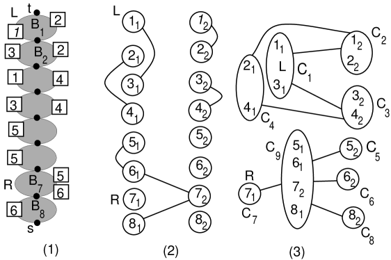
Figure 9: The graph in $($1$)$ is ${\rm pert}(\chi)$ for an S-node $\chi$, the graph in $($2$)$ is $D$, and that in $($3$)$ is $RD$.

Example 1

In Figure 9, ${\rm pert}(\chi)$ has 8 blocks $B_{1},\ldots,B_{8}$. The left side of each $B_{k}$ is ${\rm side}_{1}(B_{k})$. Also, ${\rm fam}(\chi)=\{{\cal C}_{1},\ldots,{\cal C}_{6}\}$. An integer $i$ in a small square on ${\rm side}_{p}(B_{k})$ for $p=1$ or 2 indicates that $k_{p}$ is on $P_{i}$. For example, the points on $P_{5}$ are $5_{1}$, $6_{1}$, and $7_{2}$. The letter $L$ is marked on ${\rm side}_{1}(B_{1})$, indicating that ${\rm side}_{1}(B_{1})$ must face left. The letter $R$ is marked on ${\rm side}_{1}(B_{7})$, indicating that ${\rm side}_{1}(B_{7})$ must face right. $D$ is shown in Figure 9(2). $1_{1}$ is an $L$-point while $7_{1}$ is an R-point. $RD$ is shown in Figure 9(3). $C_{1}$ is an $L$-cluster and $C_{7}$ is an R-cluster. $RD$ is bipartite and $V_{RD}$ can be partitioned into $V_{RD}^{L}=\{C_{1},C_{4},C_{9}\}$ and $V_{RD}^{R}=\{C_{2},C_{3},C_{5},C_{6},C_{7},C_{8}\}$. Thus $V_{D}^{L}=\{1_{1},2_{1},3_{1},4_{1},5_{1},6_{1},7_{2},8_{1}\}$ and $V_{D}^{R}=\{1_{2},2_{2},3_{2},4_{2},5_{2},6_{2},7_{1},8_{2}\}$. Flipping $B_{7}$ in Figure 9(1) gives a satisfying embedding of ${\rm pert}(\chi)$. If $8_{2}$ were also on $P_{5}$, there would be an edge $\{7_{2},8_{2}\}$ in $D$, which would cause $C_{9}$ and $C_{8}$ to be merged in $RD$ with a self-loop attached to it. In that case, $RD$ would not be bipartite and the CFE algorithm would output “no”.

6.3.2 $\mu$ is an R-node

In this case, adding the edge $(s,t)$ to ${\rm ske}(\mu)$ yields a simple triconnected graph. Thus, the unique embedding of ${\rm ske}(\mu)$ with both $s$ and $t$ on the exterior face is ${\rm ske}(\mu)$ itself. Let $\chi_{1}$,…, $\chi_{b}$ be the children of $\mu$ in $T$. For each $k\in\{1,\ldots,b\}$, let $B_{k,1}$,…, $B_{k,s_{k}}$ be the minor blocks of ${\rm pert}(\mu)$ in ${\rm pert}(\chi_{k})$. Note that $s_{k}=1$ when $\chi_{k}$ is an R-node or P-node. To process $\mu$, the CFE algorithm proceeds in five stages:

$\bullet$ Stage R1 first computes ${\cal C}^{\prime}_{i}=\{{\rm img}(U_{i,j},\mu)~{}|~{}U_{i,j}\in{\cal C}_{i}\}$ for every ${\cal C}_{i}\in{\rm fam}(\mu)$. Let ${\cal M}^{\prime}(\mu)$ be the sequence of all ${\cal C}^{\prime}_{i}$ with ${\cal C}_{i}\in{\rm fam}(\mu)$. Then R1 calls Theorem 3.8(2) to solve the CFE problem on input ${\rm ske}(\mu)$ and ${\cal M}^{\prime}(\mu)$. If the output is “no”, R1 outputs “no” and stops. Otherwise, for each ${\cal C}^{\prime}_{i}$ in ${\cal M}^{\prime}(\mu)$, there is a face $F_{i}$ in ${\rm ske}(\mu)$ whose boundary intersects each ${\rm img}(U_{i,j},\mu)\in{\cal C}^{\prime}_{i}$. Note that $F_{i}$ must be unique or else ${\rm done}({\cal C}_{i})$ would be a descendent of $\mu$, contradicting the fact ${\cal C}_{i}\in{\rm fam}(\mu)$.

$\bullet$ Stage R2 computes the minor block $B_{k,l}$ of ${\rm pert}(\mu)$ strictly containing $U_{i,j}$ for each ${\cal C}_{i}\in{\rm fam}(\mu)$ and each type-4 $U_{i,j}\in{\cal C}_{i}$. If $U_{i,j}$ is two-sided for $B_{k,l}$, either side of $B_{k,l}$ may be embedded toward the face $F_{i}$; otherwise, for some $p\in\{1,2\}$, $U_{i,j}$ is side-$p$ for $B_{k,l}$ and it requires that ${\rm side}_{p}(B_{k,l})$ be embedded towards $F_{i}$.

$\bullet$ Stage R3 makes sure that for every ${\cal C}_{i}$ straddling ${\rm pert}(\mu)$ and for every $U_{i,j}\in{\cal C}_{i}$ strictly contained in ${\rm pert}(\mu)$, a vertex in $U_{i,j}$ is embedded on the exterior face of ${\rm pert}(\mu)$. This is done by checking whether the following statements are all false.

1. There are an exterior edge $e_{k}$ of ${\rm ske}(\mu)$ and a minor block $B_{k,l}$ of ${\rm pert}(\mu)$ on $e_{k}$ with $\max_{p\in\{1,2\}}{\rm ext}_{p}(B_{k,l})<0pt(\mu)$; thus, both ${\rm side}_{1}(B_{k,l})$ and ${\rm side}_{2}(B_{k,l})$ must be embedded towards the exterior face of ${\rm ske}(\mu)$.

2. There are an interior edge $e_{k}$ of ${\rm ske}(\mu)$ and a minor block $B_{k,l}$ of ${\rm pert}(\mu)$ on $e_{k}$ with $\min_{p\in\{0,1,2\}}{\rm ext}_{p}(B_{k,l})<0pt(\mu)$; thus, at least one of ${\rm side}_{1}(B_{k,l})$ and ${\rm side}_{2}(B_{k,l})$ must be embedded towards the exterior face of ${\rm ske}(\mu)$.

3. There is a $U_{i,j}\in{\rm sub}(\mu)$ with $0pt({\rm done}({\cal C}_{i}))<0pt(\mu)$ (i.e., ${\cal C}_{i}$ straddles ${\rm pert}(\mu)$) and neither side of ${\rm ske}(\mu)$ contains an image in ${\rm img}(U_{i,j},\mu)$.

4. There are an S-child $\chi_{k}$ of $\mu$ and a $U_{i,j}\in{\rm sub}(\chi_{k})$ such that $0pt({\rm done}({\cal C}_{i}))<0pt(\mu)$ and the virtual edge $e_{k}$ of $\chi_{k}$ is an interior edge in ${\rm ske}(\mu)$.

If at least one statement above holds, R3 outputs “no” and stops. Otherwise, for each minor block $B_{k,l}$ of ${\rm pert}(\mu)$ such that ${\rm ext}_{p}(B_{k,l})<0pt(\mu)$ for some $p\in\{1,2\}$, it requires that ${\rm side}_{p}(B_{k,l})$ be embedded towards the exterior face of ${\rm ske}(\mu)$. Note that since the above 2 is false, the representative $e_{k}$ of $B_{k,l}$ in ${\rm ske}(\mu)$ must be an exterior edge of ${\rm ske}(\mu)$.

$\bullet$ Stage R4 first checks whether for some minor block $B_{k,l}$ of ${\rm pert}(\mu)$, the orientation requirements imposed on $B_{k,l}$ in Stage R2 or R3 are in conflict. If they are, R4 outputs “no” and stops. Otherwise, for each R-child or P-child $\chi_{k}$ of $\mu$, the minor block ${\rm pert}(\chi_{k})$ can be oriented according to the requirements imposed on it, or arbitrarily if no requirement was imposed on it. Afterwards, for each S-child $\chi_{k}$ of $\mu$, it calls the S-procedure on input $\chi_{k}$ together with the orientation requirements that were imposed on the minor blocks in ${\rm pert}(\chi_{k})$ in Stage R2 or R3. If the S-procedure on a $\chi_{k}$ outputs “no”, R4 outputs “no” and stops because ${\rm pert}(\chi_{k})$ cannot be successfully embedded; otherwise, it has found a satisfying embedding of ${\rm pert}(\mu)$.

$\bullet$ Stage R5 computes ${\rm ext}_{p}({\rm pert}(\mu))$ for $p=0$, 1, 2 as follows. Let ${\rm xsub}^{\prime}(\mu)=\{U_{i,j}\in{\rm xsub}(\mu)~{}|$ $0pt({\rm done}({\cal C}_{i}))<0pt(\mu)\}$; i.e., ${\rm xsub}^{\prime}(\mu)$ consists of all $U_{i,j}\in{\rm xsub}(\mu)$ such that ${\cal C}_{i}$ straddles ${\rm pert}(\mu)$. Partition ${\rm xsub}^{\prime}(\mu)$ into $A_{0}$, $A_{1}$, $A_{2}$ where $A_{0}$ (respectively, $A_{1}$ or $A_{2}$) consists of all $U_{i,j}\in{\rm xsub}^{\prime}(\mu)$ such that $U_{i,j}$ is two-sided (respectively, side-1 or side-2) for ${\rm pert}(\mu)$. For $i\in\{1,2\}$, let $\beta_{i}=\min_{p,B_{k,l}}{\rm ext}_{p}(B_{k,l})$ where $p$ ranges over all integers in $\{0,1,2\}$ and $B_{k,l}$ ranges over all minor blocks on an edge of ${\rm side}_{i}({\rm ske}(\mu))$. Then, set

$${\rm ext}_{0}({\rm pert}(\mu)) = \min_{U_{i,j}\in A_{0}}0pt({\rm done}({\cal C}_{i}));$$

$${\rm ext}_{1}({\rm pert}(\mu)) = \min\{\beta_{1},\min_{U_{i,j}\in A_{1}}0pt({\rm done}({\cal C}_{i}))\};$$

$${\rm ext}_{2}({\rm pert}(\mu)) = \min\{\beta_{2},\min_{U_{i,j}\in A_{2}}0pt({\rm done}({\cal C}_{i}))\}.$$

This completes the processing of $\mu$.

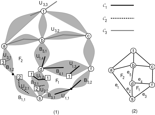
Figure 10: The graph in $($1$)$ is ${\rm pert}(\mu)$ for an R-node $\mu$, and the graph in $($2$)$ is ${\rm ske}(\mu)$.

Example 2

In Figure 10, the circles denote the vertices in ${\rm ske}(\mu)$, where $s$ and $t$ are the poles of ${\rm pert}(\mu)$. An integer $i$ in a small square at a side of a block $B_{k,l}$ indicates that a set in ${\cal C}_{i}$ has a vertex on that side of $B_{k,l}$. Also, ${\rm fam}(\mu)=\{{\cal C}_{1},{\cal C}_{2}\}$. ${\cal C}_{1}=\{U_{1,1},\ldots,U_{1,4}\}$. $U_{1,1}$ is of type 3 and ${\rm img}(U_{1,1},\mu)=\{e_{3}\}$. $U_{1,2}$ and $U_{1,3}$ are of type 4, ${\rm img}(U_{1,2},\mu)=\{e_{2}\}$, and ${\rm img}(U_{1,3},\mu)=\{e_{4}\}$. $U_{1,2}$ is two-sided for $B_{2,1}$. $U_{1,4}$ is of type 2 and ${\rm img}(U_{1,4},\mu)=\{d\}$. ${\cal C}_{2}$ consists of $U_{2,1}$ and $U_{2,2}$, which are of type 4. ${\rm img}(U_{2,1},\mu)=\{e_{1}\}$ and ${\rm img}(U_{2,2},\mu)=\{e_{2}\}$. ${\cal C}_{3}$ is the only family straddling ${\rm pert}(\mu)$. $U_{3,1}$, $U_{3,2}$, and $U_{3,3}$ are the sets in ${\cal C}_{3}$ that intersect ${\rm pert}(\mu)$; the other sets in ${\cal C}_{3}$ are not shown in this figure. $U_{3,1}$ is of type 4 and ${\rm img}(U_{3,1},\mu)=\{e_{1}\}$. $U_{3,2}$ is of type 2 and is two-sided for ${\rm pert}(\mu)$; ${\rm img}(U_{3,2},\mu)=\{a,b,c\}$. Since $U_{3,3}$ is not strictly contained in ${\rm pert}(\mu)$, it is not tested during the processing of $\mu$. Note that ${\rm pert}(\mu)$ has a satisfying embedding as shown. For $i=1,2$, the boundary of $F_{i}$ intersects each set in ${\cal C}_{i}$. The exterior face of ${\rm pert}(\mu)$ contains an image of every set in ${\cal C}_{3}$ strictly contained in ${\rm pert}(\mu)$. The side of $B_{4,1}$ on which $1$ is marked must be embedded toward $F_{1}$. In contrast, whichever side of $B_{2,1}$ is embedded toward $F_{1}$, the boundary of $F_{1}$ intersects $U_{1,2}$. In the embedding of ${\rm pert}(\mu)$, ${\cal C}_{3}$ is side-1 (respectively, side-0) exterior-forcing for ${\rm pert}(\mu)$ because of $U_{3,1}$ (respectively, $U_{3,2}$).

6.3.3 $\mu$ is a P-node

In this case, ${\rm ske}(\mu)$ consists of parallel edges $e_{1},e_{2},\ldots,e_{b}$ between its two poles with $b\geq 2$. Let $\chi_{1}$,…, $\chi_{b}$ be the children of $\mu$ in $T$. For each $k\in\{1,\ldots,b\}$, let $B_{k,1}$,…, $B_{k,s_{k}}$ be the minor blocks of ${\rm pert}(\mu)$ in ${\rm pert}(\chi_{k})$. When embedding ${\rm ske}(\mu)$, edges $e_{1}$ through $e_{b}$ can be embedded in any order. The CFE algorithm first finds a proper embedding of ${\rm ske}(\mu)$ in three stages:

$\bullet$ Stage P1 constructs an auxiliary graph $H=(V_{H},E_{H})$ with $V_{H}=\{e_{1},\ldots,e_{b}\}$ by performing the following steps in turn for every ${\cal C}_{i}\in{\rm fam}(\mu)$:

1. Compute $S_{i}=\cup_{U_{i,j}}{\rm img}(U_{i,j},\mu)$, where $U_{i,j}$ ranges over all type-3 or type-4 sets in ${\cal C}_{i}$. Let $m_{i}$ be the number of edges in $S_{i}$. Then, $m_{i}\geq 2$; otherwise ${\cal C}_{i}$ would be in ${\rm fam}(\chi_{k})$ for some $k\in\{1,\ldots,b\}$.

2. If $m_{i}\geq 3$, then output “no” and stop since ${\rm pert}(\mu)$ does not satisfy ${\cal C}_{i}$.

3. Insert edge $\{e_{k},e_{k^{\prime}}\}$ to $H$, where $e_{k}$ and $e_{k^{\prime}}$ are the two edges in $S_{i}$.

Note that for each ${\cal C}_{i}\in{\rm fam}(\mu)$, no set in ${\cal C}_{i}$ is of type 2, and each type-1 set in ${\cal C}_{i}$ contains a pole of ${\rm pert}(\mu)$, which is on every face of all embeddings of ${\rm ske}(\mu)$. For this reason, neither type-1 nor type-2 set in ${\cal C}_{i}$ is considered in the construction of $H$.

$\bullet$ Stage P2 checks whether both statements below are false in order to ensure that for every ${\cal C}_{i}$ straddling ${\rm pert}(\mu)$ and every $U_{i,j}\in{\cal C}_{i}$ strictly contained in ${\rm pert}(\mu)$, a vertex in $U_{i,j}$ is embedded on the exterior face of ${\rm pert}(\mu)$.

1. There is a minor block $B_{k,l}$ of ${\rm pert}(\mu)$ with $\max_{p\in\{1,2\}}{\rm ext}_{p}(B_{k,l})<0pt(\mu)$.

2. There are at least three edges $e_{k}$ in ${\rm ske}(\mu)$ such that (1) there is a minor block $B_{k,l}$ on $e_{k}$ with $\min_{p\in\{0,1,2\}}{\rm ext}_{p}(B_{k,l})<0pt(\mu)$; or (2) $\chi_{k}$ is an S-node and there exists $U_{i,j}$ in ${\rm sub}(\chi_{k})$ with $0pt({\rm done}({\cal C}_{i}))<0pt(\mu)$.

If Statement 1 or 2 holds, P2 outputs “no” and stops. Otherwise, it marks each $e_{k}\in V_{H}$ for which Statement 2(a) or 2(b) holds. Note that at most two $e_{k}\in V_{H}$ are marked, and each marked $e_{k}\in V_{H}$ must be an exterior edge in any satisfying embedding of ${\rm ske}(\mu)$.

$\bullet$ Stage P3 outputs “no” and stops if an $e_{k}\in V_{H}$ has degree at least three in $H$ or a marked $e_{k}\in V_{H}$ has degree 2 in $H$. Otherwise, P3 finds and fixes an embedding of ${\rm ske}(\mu)$ where (1) each marked $e_{k}\in V_{H}$ is in the exterior face and (2) for every $\{e_{k},e_{k^{\prime}}\}\in E_{H}$, $e_{k}$ and $e_{k^{\prime}}$ form the boundary of a face. For each ${\cal C}_{i}\in{\rm fam}(\mu)$, let $F_{i}$ be the face in the fixed embedding of ${\rm ske}(\mu)$ whose boundary is formed by the two edges in $S_{i}$. Note that for each $U_{i,j}\in{\cal C}_{i}$, the boundary of $F_{i}$ intersects ${\rm img}(U_{i,j},\mu)$.

Next, the CFE algorithm tries to embed ${\rm pert}(\mu)$ based on the embedding of ${\rm ske}(\mu)$ fixed in Stage P3 through the same stages as Stages R2 through R5 in §6.3.2 except that in the stage corresponding to R5, $A_{0}=\emptyset$ and the algorithm sets ${\rm ext}_{0}({\rm pert}(\mu))=\infty$. This completes the processing of $\mu$.

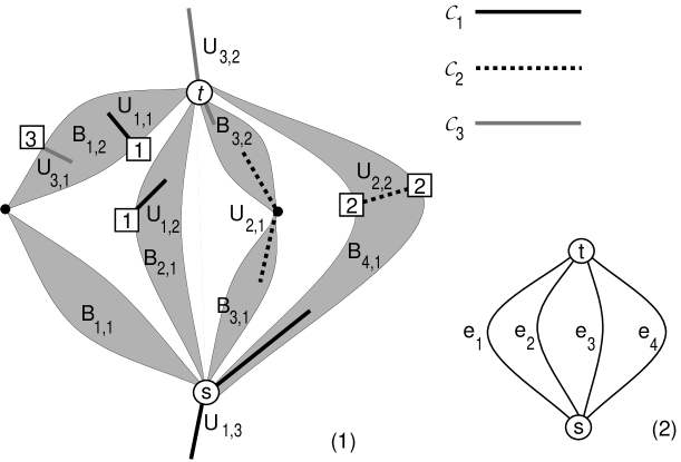
Figure 11: The graph in $($1$)$ is ${\rm pert}(\mu)$ for a P-node $\mu$, and that in $($2$)$ is ${\rm ske}(\mu)$.

Example 3

In Figure 11, ${\rm fam}(\mu)=\{{\cal C}_{1},{\cal C}_{2}\}$. ${\cal C}_{1}=\{U_{1,1},U_{1,2},U_{1,3}\}$. Both $U_{1,1}$ and $U_{1,2}$ are of type 4; ${\rm img}(U_{1,1},\mu)=\{e_{1}\}$ and ${\rm img}(U_{1,2},\mu)=\{e_{2}\}$. $U_{1,3}$ is of type 1 and needs not be tested during the processing of $\mu$. ${\cal C}_{2}=\{U_{2,1},U_{2,2}\}$. $U_{2,1}$ is of type 3 and ${\rm img}(U_{2,1},\mu)=\{e_{3}\}$. $U_{2,2}$ is of type 4 and ${\rm img}(U_{2,2},\mu)=\{e_{4}\}$. ${\cal C}_{3}$ is the only family straddling ${\rm pert}(\mu)$. $\{U_{3,1}$ and $U_{3,2}\}$ are the sets in ${\cal C}_{3}$ that intersect ${\rm pert}(\mu)$; the other sets in ${\cal C}_{3}$ are not shown in this figure. Since $U_{3,2}$ contains the pole $t$ of ${\rm pert}(\mu)$, it is not tested during the processing of $\mu$. $U_{3,1}$ is of type 4 and ${\rm img}(U_{3,1},\mu)=\{e_{1}\}$. $V_{H}=\{e_{1},e_{2},e_{3},e_{4}\}$ and $E_{H}=\{\{e_{1},e_{2}\},\{e_{3},e_{4}\}\}$. Only $e_{1}$ is marked in graph $H$. Figure 11(2) shows an embedding of ${\rm ske}(\mu)$ that might be found and fixed in Stage P3. This embedding of ${\rm ske}(\mu)$ results in a satisfying embedding of ${\rm pert}(\mu)$ as shown. If either ${\cal C}_{1}$ had another set strictly contained in block $B_{4,1}$ or ${\cal C}_{3}$ had another set strictly contained in $B_{2,1}$, then ${\rm pert}(\mu)$ has no satisfying embedding.

This completes the description of the CFE algorithm. Its correctness follows from the above discussion and Fact 6.3.

6.4 Implementation and analysis

We implement the CFE algorithm as follows. The nodes of $T$ are identified by their pre-order numbers. At each node $\mu\in T$, we store $0pt(\mu)$ and the pre-order number of the largest node in $T_{\mu}$. Let $\chi_{1},\ldots,\chi_{b}$ be the children of $\mu$. The nodes in $T_{\chi_{1}},\ldots,T_{\chi_{b}}$ form an ordered partition of the nodes in $T_{\mu}-\{\mu\}$. For a node $\nu$, we can check whether $\nu$ is in $T_{\mu}$ in $O(1)$ time. If $\nu\in T_{\mu}$, we can find the subtree $T_{\chi_{k}}$ containing $\nu$ in $O(\log|{\cal G}|)$ time, by binary searching the children of $\mu$. We equip $T$ with a data structure which can be constructed in linear time and outputs a least common ancestor query in $O(1)$ time [16, 27].

We also store ${\rm ske}(\mu)$ at $\mu$. Each $\mu$ has a pointer to its virtual edge in its parent’s skeleton. For each non-pole vertex of ${\rm ske}(\mu)$, we mark $\mu$ as its proper allocation node. This takes $O(|{\cal G}|)$ total time by Fact 6.2(1). Each edge $e$ of ${\cal G}$ has a pointer to the leaf node in $T$ that represents $e$.

Lemma 6.4

Given ${\cal G}$, ${\cal M}$, and $T$, we can compute ${\rm fam}(\mu)$, ${\rm sub}(\mu)$, ${\rm done}({\cal C}_{i})$, and ${\rm done}(U_{i,j})$ for all nodes $\mu$ of $T$, all ${\cal C}_{i}$ in ${\cal M}$, and all $U_{i,j}$ in ${\cal C}_{i}$ in $O(I)$ total time.

Proof. For each vertex $v$ of ${\cal G}$, let ${\rm low}(v)$ be the deepest allocation node of $v$ in $T$. In $O(|{\cal G}|)$ time, we can compute ${\rm low}(v)$ for all vertices $v$ of ${\cal G}$. For a set $U_{i,j}\in{\cal C}_{i}$, if a pole of ${\cal G}$ is in $U_{i,j}$, then ${\rm done}(U_{i,j})$ is the root of $T$; otherwise, ${\rm done}(U_{i,j})$ is the least common ancestor of all ${\rm low}(v)$ with $v\in U_{i,j}$. So, ${\rm done}(U_{i,j})$ can be computed in $O(|U_{i,j}|)$ time. Let ${\rm low}(U_{i,j})$ be the deepest one among all ${\rm low}(v)$ with $v\in U_{i,j}$. We can compute ${\rm low}(U_{i,j})$ in $O(|U_{i,j}|)$ time. Since ${\rm done}({\cal C}_{i})$ is the least common ancestor of all ${\rm low}(U_{i,j})$ with $U_{i,j}\in{\cal C}_{i}$, it can be computed in $O(|{\cal C}_{i}|)$ time. Thus, in $O(I)$ total time, we can compute ${\rm done}(U_{i,j})$ and ${\rm done}({\cal C}_{i})$ for all ${\cal C}_{i}$ in ${\cal M}$ and all $U_{i,j}$ in ${\cal C}_{i}$. Afterwards, in $O(I)$ total time, we can compute ${\rm fam}(\mu)$ and ${\rm sub}(\mu)$ for all nodes $\mu$ of $T$.     

After processing $\mu$, the CFE algorithm records the following information:

1. the embedding of ${\rm ske}(\mu)$;

2. ${\rm ext}_{p}({\rm pert}(\mu))$ for $p=0$, 1, and 2;

3. the edges and vertices on ${\rm side}_{1}({\rm ske}(\mu))$ and ${\rm side}_{2}({\rm ske}(\mu))$, respectively;

4. an integer $p=0$, 1 or 2, for each $U_{i,j}\in{\rm xsub}(\mu)$, indicating whether $U_{i,j}$ is two-sided, side-1, or side-2 for ${\rm pert}(\mu)$, respectively.

The CFE algorithm processes a P-node or R-node $\mu$ with the five operations below.

Operation 1 uses $O(|U_{i,j}|+\log|{\cal G}|)$ time to determine the type of a given $U_{i,j}$ in ${\rm xfam}(\mu)$ and finds ${\rm img}(U_{i,j},\mu)$ as follows. Let $\nu={\rm done}(U_{i,j})$.

Case 1: $0pt(\nu)\leq 0pt(\mu)$. Then, $U_{i,j}$ is of type 1 or 2 for ${\rm pert}(\mu)$. $U_{i,j}$ is of type 1 if and only if it contains a pole of ${\rm pert}(\mu)$. Also, ${\rm img}(U_{i,j},\mu)$ consists of all $v\in U_{i,j}$ which are also in ${\rm ske}(\mu)$. Note that $v\in{\rm ske}(\mu)$ if and only if $\mu$ is the proper allocation node of $v$ or $v$ is a pole of ${\rm pert}(\mu)$.

Case 2: $0pt(\nu)=0pt(\mu)+1$ and $\nu$ is an S-node. Then, $U_{i,j}$ is of type 3 for ${\rm pert}(\mu)$. Also, ${\rm img}(U_{i,j},\mu)$ consists of the virtual edge of $\nu$ in ${\rm ske}(\mu)$.

Case 3: otherwise. Then, $U_{i,j}$ is of type-4 for ${\rm pert}(\mu)$. Also, ${\rm img}(U_{i,j},\mu)$ is the virtual edge of $\chi_{k}$ in ${\rm ske}(\mu)$, where $\chi_{k}$ is the child of $\mu$ such that $\nu$ is in the subtree $T_{\chi_{k}}$.

Operation 2 checks in $O(|U_{i,j}|)$ time whether a given $U_{i,j}\in{\rm xsub}(\mu)$ has a vertex on either side of ${\rm pert}(\mu)$ after an embedding of ${\rm pert}(\mu)$ is fixed. If $U_{i,j}\in{\rm sub}(\mu)$, we check whether a vertex in ${\rm img}(U_{i,j},\mu)$ is on either side of ${\rm ske}(\mu)$. If $U_{i,j}\in{\rm sub}(\chi_{k})$ for an S-child $\chi_{k}$ of $\mu$, we check whether the virtual edge $e_{k}$ of $\chi_{k}$ is on either side of ${\rm ske}(\mu)$.

Operation 3 uses $O(1)$ time to check whether a given $U_{i,j}\in{\rm xsub}(\mu)$ is in ${\rm xsub}^{\prime}(\mu)$ by checking whether $0pt({\rm done}({\cal C}_{i}))<0pt(\mu)$.

Operation 4 checks whether a given $U_{i,j}$ is strictly contained in ${\rm pert}(\mu)$ and if so, further computes the minor block $B$ of ${\rm pert}(\mu)$ strictly containing $U_{i,j}$ in $O(|U_{i,j}|+\log|{\cal G}|)$ total time. For the first task, we check whether (1) $\nu={\rm done}(U_{i,j})$ is a descendent of $\mu$, or (2) $\nu=\mu$ and $U_{i,j}$ contains no pole of ${\rm pert}(\mu)$. For the second task, we first find the child $\chi_{k}$ of $\mu$ such that $T_{\chi_{k}}$ contains $\nu$. If $\chi_{k}$ is not an S-node, ${\rm pert}(\chi_{k})$ is $B$; otherwise, $B$ is ${\rm pert}(\eta)$ where $\eta$ is the child of $\chi_{k}$ such that $T_{\eta}$ contains $\nu$.

Operation 5 checks in $O(\log|{\cal G}|)$ time whether a given type-4 $U_{i,j}$ for ${\rm pert}(\mu)$ is side-1, side-2, or two-sided for the minor block $B_{k,l}$ in ${\rm pert}(\mu)$ strictly containing $U_{i,j}$. Let $\eta={\rm node}(B_{k,l})$ and $\nu={\rm done}(U_{i,j})$. Note that $\eta$ has been processed. If $\eta=\nu$, this operation takes $O(1)$ time using the information stored for $\eta$. If $\nu$ is a descendent of $\eta$, the representative $e$ of $\nu$ in ${\rm ske}(\eta)$ can be found in $O(\log|{\cal G}|)$ time. Then, it takes $O(\log|{\cal G}|)$ time to check whether $e$ is on ${\rm side}_{1}({\rm ske}(\eta))$ or ${\rm side}_{2}({\rm ske}(\eta))$ using the information stored for $\eta$.

Lemma 6.5

1. $\{{\rm xfam}(\mu)~{}|~{}\mu$ is a P-node or R-node} is a partition of $\{{\cal C}_{1},\ldots,{\cal C}_{q}\}$.

2. $\{{\rm xsub}(\mu)~{}|~{}\mu$ is a P-node or R-node} is a partition of ${\cal C}_{1}\cup\cdots\cup{\cal C}_{q}$.

3. Each input family ${\cal C}_{i}$ is processed exactly once.

4. Each input $U_{i,j}$ is processed at most twice, and the total time spent on processing $U_{i,j}$ is $O(|U_{i,j}|+\log|{\cal G}|)$.

Proof. Statements 1 and 2 are straightforward. Statement 3 holds since each ${\cal C}_{i}$ is processed only when the node $\mu$ with ${\cal C}_{i}\in{\rm xfam}(\mu)$ is processed. Each $U_{i,j}$ is processed once when the node $\mu$ with $U_{i,j}\in{\rm xsub}(\mu)$ is processed and once when the node $\phi$ with ${\cal C}_{i}\in{\rm xfam}(\phi)$ is processed. When $U_{i,j}$ is processed, we perform some of Operations 1 through 5 on it. Since an operation takes $O(|U_{i,j}|+\log|{\cal G}|)$ time, Statement 4 holds.     

We now bound the time of processing an R-node or P-node $\mu$. Let ${\rm xske}(\mu)$ be obtained from ${\rm ske}(\mu)$ by replacing the virtual edge of each S-child $\chi_{k}$ of $\mu$ with ${\rm ske}(\chi_{k})$. Let $n_{\mu}$ be the number of vertices in ${\rm xske}(\mu)$. Let $N_{\mu}=\sum_{{\cal C}_{i}\in{\rm xfam}(\mu)}|{\cal C}_{i}|$. Recall that $\mu$ is processed using some of the following operations:

1. Process the sets $U_{i,j}$ in the families ${\cal C}_{i}\in{\rm xfam}(\mu)$.

2. Call Theorem 3.8(2) on input ${\rm ske}(\mu)$ and ${\cal M}^{\prime}(\mu)$.

3. Call the S-procedure on $\chi_{k}$ for the S-children $\chi_{k}$ of $\mu$.

4. Compute ${\rm ext}_{p}({\rm pert}(\mu))$ for $p=0$, 1, and 2.

5. Construct auxiliary graphs $D$, $RD$ and $H$, and operate on them.

Note that each $K\in\{D,RD,H\}$ is constructed and operated on in $O(|K|)$ total time. Since $\sum_{K}|K|\leq n_{\mu}$ where $K$ ranges over all auxiliary graphs constructed during the processing of $\mu$, it takes $O(n_{\mu})$ total time to process the auxiliary graphs for $\mu$. Therefore, the above operations take $O((n_{\mu}+N_{\mu})\log I)$ time in total. By summing over all P-nodes and R-nodes $\mu$ of $T$, and by Theorem 3.8, Fact 6.2(1), and Lemma 6.5, the CFE algorithm runs in the desired total time, completing the proof of Theorem 6.1.

7 Directions for further research

We have proved that the CFE problem can be solved in $O(I\log I)$ time for the special case where for each input family ${{\cal C}}_{i}$, each set in ${{\cal C}}_{i}$ induces a connected subgraph of the input graph ${\cal G}$. One direction for further research would be to reduce the running time to linear. Such a result might lead to substantial simplification of the SPQR decomposition or an entirely different data structure. Another worthy direction would be to solve more general cases in similar time bounds. Beyond these technical open problems, it would be of significance to find further applications of the CFE problem than VLSI layout and topological inference as well as to identify novel and fundamental constrained planar embeddings.

References

- [1] G. D. Battista and R. Tamassia. On-line graph algorithms with SPQR-trees. Algorithmica, 15:302–318, 1996.
- [2] G. D. Battista and R. Tamassia. On-line planarity testing. SIAM J. Comput., 25(5):956–997, 1996.
- [3] D. Bienstock and C. L. Monma. On the complexity of covering vertices by faces in a planar graph. SIAM Journal on Computing, 17(1):53–76, 1988.
- [4] K. Booth and G. Lueker. Testing for the consecutive ones property, interval graphs, and graph planarity using PQ-tree algorithms. Journal of Computer and System Sciences, 13:335–379, 1976.
- [5] J. Boyer and W. Myrvold. Stop minding your P’s and Q’s: A simplified planar embedding algorithm. In Proceedings of the 10th Annual ACM-SIAM Symposium on Discrete Algorithms, 1999. To appear.
- [6] Z.-Z. Chen, M. Grigni, and C. H. Papadimitriou. Planar map graphs. In Proceedings of the 30th Annual ACM Symposium on Theory of Computing, pages 514–523, 1998.
- [7] Z. Z. Chen, X. He, and M. Y. Kao. Nonplanar topological inference and political-map graphs. In Proceedings of the 10th Annual ACM-SIAM Symposium on Discrete Algorithms, pages 195–204, 1999.
- [8] M. J. Egenhofer. Reasoning about binary topological relations. In O. Gunther and H. J. Schek, editors, Proc. Advances in Spatial Database (SSD’91), pages 143–160, 1991.
- [9] M. J. Egenhofer and J. Sharma. Assessing the consistency of complete and incomplete topological information. Geographical Systems, 1:47–68, 1993.
- [10] G. Ehrlich, S. Even, and R. E. Tarjan. Intersection graphs of curves in the plane. Combinatorial Theory Ser. B, 21(1:):8–20, 1976.
- [11] R. E. Erickson, C. L. Monma, and A. F. Veinott, Jr. Send-and-split method for minimum-concave-cost network flows. Mathematics of Operations Research, 12(4):634–664, 1987.
- [12] S. Even and R. E. Tarjan. Computing an -numbering. Theoretical Computer Science, 2:339–344, 1976.
- [13] G. N. Frederickson. Using cellular graph embeddings in solving all pairs shortest paths problems. Journal of Algorithms, 19(1):45–85, 1995.
- [14] M. Garey and D. Johnson. Computers and Intractability: A Guide to the Theory of NP-Completeness. Freeman, New York, NY, 1979.
- [15] M. Grigni, D. Papadias, and C. H. Papadimitriou. Topological inference. In Proc. 14th IJCAI, pages 901–906, 1995.
- [16] D. Harel and R. E. Tarjan. Fast algorithms for finding nearest common ancestors. SIAM Journal on Computing, 13:338–355, 1984.
- [17] G. Kant and X. He. Regular edge labeling of 4-connected plane graphs and its applications in graph drawing problems. Theoretical Computer Science, 172:175–193, 1997.
- [18] M. Y. Kao, M. Fürer, X. He, and B. Raghavachari. Optimal parallel algorithms for straight-line grid embeddings of planar graphs. SIAM Journal on Discrete Mathematics, 7(4):632–646, 1994.
- [19] B. Mohar. Embedding graphs in an arbitrary surface in linear time. In Proceedings of the 28th Annual ACM Symposium on Theory of Computing, pages 392–397, 1996.
- [20] J. Nešetřil and M. Rosenfeld. Embedding graphs in Euclidean spaces, an exploration guided by Paul Erdős. Geombinatorics, 6(4):143–155, 1997.
- [21] T. Nishizeki and N. Chiba. Planar Graphs: Theory and Algorithms. North-Holland, 1988.
- [22] O. Ore. The Four-Color Problem. Academic Press, 1967.
- [23] D. Papadias and T. Sellis. The qualitative representation of spatial knowledge in two-dimensional space. Very Large Data Bases Journal, 4:479–516, 1994.
- [24] C. H. Papadimitriou, D. Suciu, and V. Vianu. Topological queries in spatial databases. In Proc. 1996 PODS, 1996.
- [25] J. S. Provan. Convexity and the Steiner tree problem. Networks, 18(1):55–72, 1988.
- [26] V. Ramachandran and J. Reif. Planarity testing in parallel. Journal of Computer and System Sciences, 49(3):517–561, Dec. 1994.
- [27] B. Schieber and U. Vishkin. On finding lowest common ancestors: Simplification and parallelization. SIAM Journal on Computing, 17(6):1253–1262, Dec. 1988.
- [28] D. D. Sleator and R. E. Tarjan. Self-adjusting binary search tree. Journal of the ACM, 32:652–686, 1985.
- [29] I. G. Tollis. Graph drawing and information visualization. ACM Computing Surveys, 28(4es):19, 1996.
- [30] H. Whitney. 2-isomorphic graphs. Amer. J. Math., 55:245–254, 1933.