Compact Encodings of Planar Graphs
via Canonical Orderings and Multiple Parentheses

Abstract

Let $G$ be a plane graph of $n$ nodes, $m$ edges, $f$ faces, and no self-loop. $G$ need not be connected or simple (i.e., free of multiple edges). We give three sets of coding schemes for $G$ which all take $O(m+n)$ time for encoding and decoding. Our schemes employ new properties of canonical orderings for planar graphs and new techniques of processing strings of multiple types of parentheses.

For applications that need to determine in $O(1)$ time the adjacency of two nodes and the degree of a node, we use $2m+{(5+\frac{1}{k})}n+o(m+n)$ bits for any constant $k>0$ while the best previous bound by Munro and Raman is $2m+8n+o(m+n)$. If $G$ is triconnected or triangulated, our bit count decreases to $2m+3n+o(m+n)$ or $2m+2n+o(m+n)$, respectively. If $G$ is simple, our bit count is $\frac{5}{3}m+{(5+\frac{1}{k})}n+o(n)$ for any constant $k>0$. Thus, if a simple $G$ is also triconnected or triangulated, then $2m+2n+o(n)$ or $2m+n+o(n)$ bits suffice, respectively.

If only adjacency queries are supported, the bit counts for a general $G$ and a simple $G$ become $2m+\frac{14}{3}n+o(m+n)$ and $\frac{4}{3}m+5n+o(n)$, respectively.

If we only need to reconstruct $G$ from its code, a simple and triconnected $G$ uses $\frac{3\log_{2}3}{2}m+O(1)\approx 2.38m+O(1)$ bits while the best previous bound by He, Kao, and Lu is $2.84m$.

1 Introduction

This paper investigates the problem of encoding a given graph $G$ into a binary string $S$ with the requirement that $S$ can be decoded to reconstruct $G$. This problem has been extensively studied with three objectives: (1) minimizing the length of $S$, (2) minimizing the time needed to compute and decode $S$, and (3) supporting queries efficiently.

As these objectives are often in conflict, a number of coding schemes with different trade-offs have been proposed. The standard adjacency-list encoding of a graph is widely useful but requires $2m\lceil\log n\rceil$ bits where $m$ and $n$ are the numbers of edges and nodes, respectively. A folklore scheme uses $2n$ bits to encode a rooted $n$-node tree into a string of $n$ pairs of balanced parentheses. Since the total number of such trees is at least $\frac{1}{2(n-1)}{\cdot}\frac{(2n-2)!}{(n-1)!(n-1)!}$, the minimum number of bits needed to differentiate these trees is the log of this quantity, which is $2n-o(n)$ by Stirling’s approximation formula. Thus, two bits per edge up to an additive $o(1)$ term is an information-theoretic tight bound for encoding rooted trees. The rooted trees are the only nontrivial graph family with a known polynomial-time coding scheme whose code length matches the information-theoretic bound.

For certain graph families, Kannan, Naor and Rudich [12] gave schemes that encode each node with $O(\log n)$ bits and support $O(\log n)$-time testing of adjacency between two nodes. For dense graphs and complement graphs, Kao, Occhiogrosso, and Teng [17] devised two compressed representations from adjacency lists to speed up basic graph techniques. Galperin and Wigderson [7] and Papadimitriou and Yannakakis [22] investigated complexity issues arising from encoding a graph by a small circuit that computes its adjacency matrix. For labeled planar graphs, Itai and Rodeh [10] gave an encoding of $\frac{3}{2}n\log n+O(n)$ bits. For unlabeled general graphs, Naor [21] gave an encoding of ${\frac{1}{2}}n^{2}-n\log{n}+O(n)$ bits.

Let $G$ be a plane graph with $n$ nodes, $m$ edges, $f$ faces, and no self-loop. $G$ need not be connected or simple (i.e., free of multiple edges). We give coding schemes for $G$ which all take $O(m+n)$ time for encoding and decoding. The bit counts of our schemes depend on the level of required query support and the structure of the encoded family of graphs. In particular, whether multiple edges (or self-loops) are permitted plays a significant role.

For applications that require support of certain queries, Jacobson [11] gave an $\Theta(n)$-bit encoding for a connected and simple planar graph $G$ that supports traversal in $\Theta(\log{n})$ time per node visited. Munro and Raman [20] recently improved this result and gave schemes to encode binary trees, rooted ordered trees and planar graphs. For a general planar $G$, they used $2m+8n+o(m+n)$ bits while supporting adjacency and degree queries in $O(1)$ time. We reduce this bit count to $2m+{(5+\frac{1}{k})}n+o(m+n)$ for any constant $k>0$ with the same query support. If $G$ is triconnected or triangulated, our bit count further decreases to $2m+3n+o(m+n)$ or $2m+2n+o(m+n)$, respectively. With the same query support, we can encode a simple $G$ using only $\frac{5}{3}m+{(5+\frac{1}{k})}n+o(n)$ bits for any constant $k>0$. As a corollary, if a simple $G$ is also triconnected or triangulated, the bit count is $2m+2n+o(n)$ or $2m+n+o(n)$, respectively.

If only $O(1)$-time adjacency queries are supported, our bit counts for a general $G$ and a simple $G$ become $2m+\frac{14}{3}n+o(m+n)$ and $\frac{4}{3}m+5n+o(n)$, respectively. All our schemes mentioned so far as well as that of [20] can be modified to accommodate self-loops with $n$ additional bits.

If we only need to reconstruct $G$ with no query support, the code length can be substantially shortened. For this case, Turán [25] used $4m$ bits for $G$ that may have self-loops; this bound was improved by Keeler and Westbrook [18] to $3.58m$ bits. They also gave coding schemes for several important families of planar graphs. In particular, they used $1.53m$ bits for a triangulated simple $G$, and $3m$ bits for a connected $G$ free of self-loops and degree-one nodes. For a simple triangulated $G$, He, Kao, and Lu [9] improved the count to $\frac{4}{3}m+O(1)$. Tutte [26] gave an information-theoretic tight bound of roughly $1.08m$ bits for a triangulated $G$. For a simple $G$ that is free of self-loops, triconnected and thus free of degree-one nodes, He, Kao, and Lu [9] improved the count to at most $2.84m$. We further improve the bit count to at most $\frac{3\log 3}{2}m+O(1)$. Figure 1 summarizes our results and compares them with previous ones.

	adjacency and degree		adjacency		no query
	[20]	ours	old	ours	[18, 9]	ours
self-loops					$3.58m$
general	$2m+8n$	$2m+{(5+\frac{1}{k})}n$		$2m+\frac{14}{3}n$
simple		$\frac{5}{3}m+{(5+\frac{1}{k})}n$		$\frac{4}{3}m+5n$
degree-one free					$3m$
triconnected		$2m+3n$		$2m+3n$
simple & triconnected		$2m+2n$		$2m+2n$	$2.84m$	$\frac{3\log 3}{2}m$
triangulated		$2m+2n$		$2m+2n$
simple & triangulated		$2m+n$		$2m+n$	$\frac{4}{3}m$

Figure 1: This table compares our results with previous ones, where $n$ is the number of nodes, $m$ is the number of edges, and $k$ is a positive constant. The lower-order terms are omitted. All but row 1 assume that $G$ has no self-loop.

Our coding schemes employ two new tools. One is new techniques of processing strings of multiple types of parentheses. This generalizes the results on strings of a single type of parentheses in [20]. The other tool is new properties of canonical orderings for plane graphs. Such orderings were introduced by de Fraysseix, Pach and Pollack [5] and extended by Kant [13]. These structures and closely related ones have proven useful also for drawing plane graphs in organized and compact manners [15, 16, 23, 24].

Section 2 discusses the new tools. Section 3 describes the coding schemes that support queries. Section 4 presents the more compact coding schemes which do not support queries. The methods used in §3 and §4 are independent, and these two sections can be read in the reverse order.

Remark. Throughout this paper, for all our coding schemes, it is straightforward to verify that both encoding and decoding take linear time in the size of the input graph. Hence for the sake of conciseness, the corresponding theorems do not state this time complexity.

2 New Encoding Tools

2.1 Basics

A simple (respectively, multiple) graph is one that does not contain (respectively, may contain) multiple edges between two distinct nodes. The simple version of a multiple graph is one obtained from the multiple graph by deleting all but one copy of each edge.

In this paper, all graphs are multiple and unlabeled unless explicitly stated otherwise. Furthermore, for technical simplicity, a multiple graph is formally a simple one with positive integral edge weights, where each edge’s weight indicates its multiplicity.

The degree of a node $v$ in a graph is the number of edges, counting multiple edges, incident to $v$ in the graph. A node $v$ is a leaf of a tree $T$ if $v$ has exactly one neighbor in $T$. Since $T$ may have multiple edges, a leaf of $T$ may have a degree greater than one. We say $v$ is internal in $T$ if $v$ has more than one neighbor in $T$. See [3, 8] for other graph-theoretic terminology used in this paper.

For a given problem of size $n$, this paper uses the $\log n$-bit word model of computation in [11, 19, 20], where operations such as read, write, add and multiply on $O(\log n)$ consecutive bits take $O(1)$ time. The model can be implemented using the following techniques. If a given chunk of $O(\log n)$ consecutive bits do not fit into a single word, they can be read or written by $O(1)$ accesses of consecutive words. Basic operations can be implemented by table look-up methods similar to the Four Russian algorithm [1].

2.2 Multiple Types of Parentheses

A string is binary if it contains at most two kinds of symbols; e.g., a string of one type of parentheses is a binary string.

Fact 1 (see [2, 6])

Let $k=O(1)$. Given any strings $S_{1},S_{2},\ldots,S_{k}$ with total length $O(n)$, there exists an auxiliary binary string $\lambda$ such that

• the string $\lambda$ has $O(\log n)$ bits and can be computed in $O(n)$ time;

• given the concatenation of $\lambda,S_{1},S_{2},\ldots,S_{k}$ as input, the index of the first symbol of any given $S_{i}$ in the concatenation can be computed in $O(1)$ time.

Let $S_{1}+S_{2}+\cdots+S_{k}$ denote the concatenation of $\lambda,S_{1},S_{2},\ldots,S_{k}$ as in Fact 1.

Let $S$ be a string. Let $|S|$ be the length of $S$. Let $S[i]$ be the symbol at the $i$-th position of $S$. $S[k]$ is enclosed by $S[i]$ and $S[j]$ in $S$ if $i<k<j$. Let ${\rm select}({S,i,\Box})$ be the position of the $i$-th $\Box$ in $S$. Let ${\rm rank}({S,k,\Box})$ be the number of $\Box$’s before or at the $k$-th position of $S$. Clearly, if $k={\rm select}({S,i,\Box})$, then $i={\rm rank}({S,k,\Box})$.

Now let $S$ be a string of multiple types of parentheses. For an open parenthesis $S[i]$ and a close one $S[j]$ of the same type where $i<j$, the two match in $S$ if every parenthesis of the same type that is enclosed by them matches one enclosed by them. $S$ is balanced if every parenthesis in $S$ belongs to a matching parenthesis pair.

Here are some queries defined for $S$:

• Let ${\rm match}({S,i})$ be the position of the parenthesis in $S$ that matches $S[i]$.

• Let ${\rm first}_{k}({S,i})$ (respectively, ${\rm last}_{k}({S,i})$) be the position of the first (respectively, last) parenthesis of the $k$-th type after (respectively, before) $S[i]$.

• Let ${\rm enclose}_{k}({S,i_{1},i_{2}})$ be the positions $(j_{1},j_{2})$ of the closest matching parenthesis pair of the $k$-th type that encloses $S[i_{1}]$ and $S[i_{2}]$.

The answer to a query may be undefined; e.g., ${\rm match}({S,i})$ is undefined for some $i$ if $S$ is not balanced. If there is only one type of parentheses in $S$, the subscript $k$ in ${\rm first}_{k}({S,i})$, ${\rm last}_{k}({S,i})$, and ${\rm enclose}_{k}({S,i,j})$ may be omitted; thus, ${\rm first}({S,i})=i+1$ and ${\rm last}({S,i})=i-1$. If it is clear from the context, the parameter $S$ may also be omitted.

Fact 2 (see [4, 19, 20])

1. Let $S$ be a binary string. An auxiliary binary string $\mu_{1}(S)$ of length $o(|S|)$ is obtainable in $O(|S|)$ time such that ${\rm rank}({S,i,\Box})$ and ${\rm select}({S,i,\Box})$ can be answered from $S+\mu_{1}(S)$ in $O(1)$ time.

2. Let $S$ be a balanced string of one type of parentheses. An auxiliary binary string $\mu_{2}(S)$ of length $o(|S|)$ is obtainable in $O(|S|)$ time such that ${\rm match}({S,i})$ and ${\rm enclose}({S,i,j})$ can be answered from $S+\mu_{2}(S)$ in $O(1)$ time.

The next theorem generalizes Fact 2.

Theorem 2.1

Let $S$ be a string of $O(1)$ types of parentheses that may be unbalanced. An auxiliary $o(|S|)$-bit string $\alpha(S)$ is obtainable in $O(|S|)$ time such that ${\rm rank}({S,i,\Box})$, ${\rm select}({S,i,\Box})$, ${\rm first}_{k}({S,i})$, ${\rm last}_{k}({S,i})$, ${\rm match}({S,i})$, and ${\rm enclose}_{k}({S,i,j})$ can be answered from $S+\alpha(S)$ in $O(1)$ time.

Proof. The case of ${\rm rank}({S,i,\Box})$ and ${\rm select}({S,i,\Box})$ is a straightforward generalization of Fact 2(1). The case of ${\rm first}_{k}({S,i})$ is proved as follows. Let $f(S,i,\Box)$ be the position of the first $\Box$ after $S[i]$. Then,

$$f(S,i,\Box) = {\rm select}({S,1+{\rm rank}({S,i,\Box}),\Box});$$

$${\rm first}_{k}({S,i}) = \min\{{f(S,i,{\mbox{\tt(}}),f(S,i,{\mbox{\tt)}})}\},$$

where ( and ) are the open and close parentheses of the $k$-th type in $S$, respectively. The case of ${\rm last}_{k}({S,i})$ can be shown similarly.

To prove the case of ${\rm match}({S,i})$ and ${\rm enclose}_{k}({S,i,j})$, we first generalize Fact 2(2) for an unbalanced binary $S$. Let $R$ be the shortest balanced superstring of $S$. Let $d=|R|-|S|$. $R$ is either $S$ appended by $d$ close parentheses or $d$ open parentheses appended by $S$. Let $\beta(S)$ be $\mu_{2}(R)$ appended to $1+\lceil\log(n+1)\rceil$ bits which record $d$ and whether $S$ is a prefix or a suffix of $R$. Then, a query for $S$ can be answered from $S+\beta(S)$ in $O(1)$ time.

Now suppose that $S$ is of $\ell$ types of parentheses. Let $S_{k}$ with $1\leq k\leq\ell$ be the string obtained from $S$ as follows.

• Every open (respectively, close) parenthesis of the $k$-th type is replaced by two consecutive open (respectively, close) parentheses of the $k$-th type.

• Every parenthesis of any other type is replaced by a matching parenthesis pair of the $k$-th type.

Each $S_{k}$ is a string of length $2|S|$ using one type of parentheses. Each symbol $S_{k}[i]$ can be determined from $S[{\lfloor{i/2}\rfloor}]$ in $O(1)$ time. For example,

$S$	=	[ [ ( { ) ] ( { } } ( ] )
$S_{1}$	=	()()((()))()((()()()((()))
$S_{2}$	=	[[[[[][][]]][][][][][]]][]
$S_{3}$	=	{}{}{}{{{}{}{}{{}}}}{}{}{}

A query for $S$ can be answered by answering the queries for some $S_{k}$ as follows.

• ${\rm match}({S,i})={\lfloor{{\rm match}({S_{k},2i})/2}\rfloor}$, where $S[i]$ is a parenthesis of the $k$-th type.

• Let $i$ and $j$ be two positions. Let

  $$A = \{{2i,2i+1,{\rm match}({S_{k},2i}),{\rm match}({S_{k},2i+1})}\}\cup$$

  $$\{{2j,2j+1,{\rm match}({S_{k},2j}),{\rm match}({S_{k},2j+1})}\}.$$

  Let $i_{1}=\min A$, $j_{1}=\max A$, and $(i_{2},j_{2})={\rm enclose}({S_{k},i_{1},j_{1}})$. Then, ${\rm enclose}_{k}({S,i,j})=({\lfloor{i_{2}/2}\rfloor},{\lfloor{j_{2}/2}\rfloor})$.

Each query above on $S_{k}$ can be answered in $O(1)$ time from $S_{k}+\beta(S_{k})$. Since each symbol $S_{k}[i]$ can be determined from $S[{\lfloor{i/2}\rfloor}]$ in $O(1)$ time, the theorem holds by letting $\alpha(S)=\beta(S_{1})+\beta(S_{2})+\cdots+\beta(S_{\ell})$.        

Given $k$ strings $S_{1},\ldots,S_{k}$ of $O(1)$ types of parentheses, let $\alpha(S_{1},S_{2},\ldots,S_{k})$ denote $\alpha(S_{1})+\alpha(S_{2})+\cdots+\alpha(S_{k})$.

2.3 Encoding Trees

An encoding for a plane graph $G$ is weakly convenient if it takes linear time to reconstruct $G$; $O(1)$ time to determine the adjacency of two nodes in $G$; $O(d)$ time to determine the degree $d$ of a node; and $O(d)$ time to list the neighbors of a node of degree $d$. A weakly convenient encoding for $G$ is convenient if it takes $O(1)$ time to determine the degree of a node.

For a simple rooted tree $T$, the folklore encoding $F(T)$ is defined as follows. Initially, $F(T)$ is a balanced string of one type of parentheses representing the preordering of $T$. An open (respectively, close) parenthesis denotes a descending (respectively, ascending) edge traversal. Then, this string is enclosed by an additional matching parenthesis pair. Note that each node of $T$ corresponds to a matching parenthesis pair in $F(T)$.

Fact 3

Let $v_{i}$ be the $i$-th node in the preordering of a simple rooted tree $T$.

1. The parenthesis pair for $v_{i}$ encloses that for $v_{j}$ in $F(T)$ if and only if $v_{i}$ is an ancestor of $v_{j}$.

2. The parenthesis pair for $v_{i}$ precedes that for $v_{j}$ in $F(T)$ if and only if $v_{i}$ and $v_{j}$ are not related and $i<j$.

3. The $i$-th open parenthesis in $F(T)$ belongs to the parenthesis pair for $v_{i}$.

Fact 4 (see [20])

For a simple rooted tree $T$ of $n$ nodes, $F(T)+\mu_{1}(F(T))+\mu_{2}(F(T))$ is a weakly convenient encoding of $2n+o(n)$ bits.

Based on Theorem 2.1, we show that Fact 4 holds even if $F(T)$ is interleaved with other types of parentheses.

Theorem 2.2

Let $T$ be a simple rooted tree. Let $S$ be a string of $O(1)$ types of parentheses such that a given type of parentheses in $S$ gives $F(T)$. Then $S+\alpha(S)$ is a weakly convenient encoding of $T$.

Proof. Let the parentheses, denoted by ( and ), in $S$ used by $F(T)$ be the $k$-th type. Let $v_{1},\ldots,v_{n}$ be the preordering of $T$. Let $p_{i}={\rm select}({S,i,{\mbox{\tt(}}})$ and $q_{i}={\rm match}({S,p_{i}})$; i.e., $S[p_{i}]$ and $S[q_{i}]$ are the matching parenthesis pair corresponding to $v_{i}$ by Fact 3(3). By Theorem 2.1, each $p_{i}$ and $q_{i}$ are obtainable from $S+\alpha(S)$ in $O(1)$ time. Moreover, the index $i$ is obtainable from $p_{i}$ or $q_{i}$ in $O(1)$ time by $i={\rm rank}({S,p_{i},{\mbox{\tt(}}})={\rm rank}({S,{\rm match}({S,q_{i}}),{\mbox{\tt(}}})$. The queries for $T$ are supported as follows.

Case 1: adjacency queries. Suppose $i<j$. Then, $(p_{i},q_{i})={\rm enclose}_{k}({p_{j},q_{j}})$ if and only if $v_{i}$ is adjacent to $v_{j}$ in $T$, i.e., $v_{i}$ is the parent of $v_{j}$ in $T$.

Case 2: neighbor queries. Suppose that $v_{i}$ has degree $d$ in $T$. The neighbors of $v_{i}$ in $T$ can be listed in $O(d)$ time as follows. First, if $i\neq 1$, output $v_{j}$, where $(p_{j},q_{j})={\rm enclose}_{k}({p_{i},q_{i}})$. Then, let $p_{j}={\rm first}_{k}({p_{i}})$. As long as $p_{j}<q_{i}$, we repeatedly output $v_{j}$ and update $p_{j}$ by ${\rm first}_{k}({{\rm match}({p_{j}})})$.

Case 3: degree queries. Since $T$ is simple, the degree $d$ of $v_{i}$ in $T$ is the number of neighbors in $T$, which is obtainable in $O(d)$ time.        

The next theorem improves Theorem 2.2 and is important for our later coding schemes. A related result in [20] shows that a $k$-page graph of $n$ nodes and $m$ edges has a convenient encoding of $2m+2kn+o(m+n)$ bits. Since $T$ is a one-page graph, this result gives a longer convenient encoding for $T$ than the next theorem.

For a condition $P$, let $\delta(P)=1$, if $P$ holds; $\delta(P)=0$, otherwise.

Theorem 2.3

Let $T$ be a rooted tree of $n$ nodes, $n^{*}$ leaves and $m$ edges. Let $S+\alpha(S)$ be a weakly convenient encoding of the simple version $T_{s}$ of $T$.

1. A string $D$ of $2m-n+n^{*}$ bits is obtainable in $O(m+n)$ time such that $S+D+\alpha(S,D)$ is a convenient encoding for $T$.

2. If $T=T_{s}$, a string $D$ of $n^{*}$ bits and a string $Y$ of $n$ bits are obtainable in $O(m+n)$ time such that $S+D+\alpha(S,D,Y)$ is a convenient encoding for $T$.

Remark. In Statement 2, the convenient encoding contains $\alpha(Y)$ but not $Y$ itself, which is only used in the decoding process and is not explicitly stored. This technique is also used in our other schemes. Proof. Let $v_{1},\ldots,v_{n}$ be the preordering of $T_{s}$. Let $d_{i}$ be the degree of $v_{i}$ in $T$. We show how to use $D$ to store the information required to obtain $d_{i}$ in $O(1)$ time.

Statement 1. Let $\delta_{i}=\delta(\mbox{$v_{i}$ is internal in $T_{s}$})$. Since $S+\alpha(S)$ is a weakly convenient encoding for $T_{s}$, each $\delta_{i}$ is obtainable in $O(1)$ time from $S+\alpha(S)$. Initially, $D$ is $n$ copies of $1$. Let $b_{i}=d_{i}-1-\delta_{i}$. We add $b_{i}$ copies of $0$ right after the $i$-th 1 in $D$ for each $v_{i}$. Since the number of internal nodes in $T_{s}$ is $n-n^{*}$, the bit count of $D$ is $n+\sum_{i=1}^{n}(d_{i}-1-\delta_{i})=2m-n+n^{*}$. $D$ is obtainable from $T$ in $O(m+n)$ time. The number $b_{i}$ of 0’s right after the $i$-th 1 in $D$ is ${\rm select}({D,i+1,\mbox{1}})-{\rm select}({D,i,\mbox{1}})-1$. Since $d_{i}=1+\delta_{i}+b_{i}$, the degree of $v_{i}$ in $T$ can be computed in $O(1)$ time from $S+D+\alpha(S,D)$.

Statement 2. Let $n_{2}$ be the number of nodes of degree two in $T$. Initially, $D$ is $n-n^{*}-n_{2}$ copies of $1$, one for each node of degree at least three in $T$. Suppose that $v_{i}$ is the $h_{i}$-th node in $v_{1},\ldots,v_{n}$ of degree at least three. We put $d_{i}-3$ copies of $0$ right after the $h_{i}$-th 1 in $D$. The bit count of $D$ is $(n-n^{*}-n_{2})+\sum_{i,d_{i}\geq 3}(d_{i}-3)=(n-n^{*}-n_{2})+(\sum_{i=1}^{n}d_{i}-n^{*}-2n_{2})-3(n-n^{*}-n_{2})=n^{*}-2<n^{*}$.

Since $S+\alpha(S)$ is a weakly convenient encoding for $T$, it takes $O(1)$ time to determine whether $d_{i}\geq 3$ from $S+\alpha(S)$. If $d_{i}<3$, $d_{i}$ can also be computed in $O(1)$ time from $S+\alpha(S)$. To compute $d_{i}$ when $d_{i}\geq 3$, note that since $d_{i}=3+{\rm select}({D,h_{i}+1,\mbox{1}})-{\rm select}({D,h_{i},\mbox{1}})-1$, it suffices to compute $h_{i}$ in $O(1)$ time. Let $Y$ be an $n$-bit string such that $Y[i]=1$ if and only if $d_{i}\geq 3$. Then, $h_{i}={\rm rank}({Y,i,\mbox{1}})$, obtainable in $O(1)$ time from $Y+\alpha(Y)$. Each symbol $Y[i]$ can be determined from $S+\alpha(S)$ in $O(1)$ time, and we do not need to store $Y$ in our encoding.        

2.4 Canonical Orderings

This section reviews canonical orderings of plane graphs [5, 13] and proves new properties needed in our coding schemes.

All graphs in this section are simple. Let $G$ be a plane graph. Let $v_{1},v_{2},\ldots,v_{n}$ be an ordering of the nodes of $G$. Let $G_{i}$ be the subgraph of $G$ induced by $v_{1},v_{2},\ldots,v_{i}$. Let $H_{i}$ be the boundary of the exterior face of $G_{i}$. This ordering is canonical if the interval $[3,n]$ can be partitioned into $I_{1},\ldots,I_{K}$ with the following properties for each $I_{j}$. Suppose $I_{j}=[k,k+q]$. Let $C_{j}$ be the path $v_{k},v_{k+1},\ldots,v_{k+q}$.

• $G_{k+q}$ is biconnected. $H_{k+q}$ contains the edge $(v_{1},v_{2})$ and $C_{j}$. $C_{j}$ has no chord in $G$.

  Remark. Since $H_{k+q}$ is a cycle, to enhance visual intuitions, we draw its nodes in the clockwise order from left to right above the edge $(v_{1},v_{2})$.

• If $q=0$, $v_{k}$ has at least two neighbors in $G_{k-1}$, all on $H_{k-1}$. If $q>0$, $C_{j}$ has exactly two neighbors in $G_{k-1}$, both on $H_{k-1}$, where the left neighbor is incident to $C_{j}$ only at $v_{k}$ and the right neighbor only at $v_{k+q}$.

  Remark. Whether $q=0$ or not, let $v_{\ell}$ and $v_{r}$ denote the leftmost neighbor and the rightmost neighbor of $C_{j}$ on $H_{k-1}$.

• For each $v_{i}$ where $k\leq i\leq k+q$, if $i<n$, $v_{i}$ has at least one neighbor in $G-G_{k+q}$.

Figure 2 shows a canonical ordering of a triconnected plane graph; Figure 3(1) illustrates one for a plane triangulation.

Fact 5 (see [5, 13])

1. If $G$ is triconnected or triangulated, then it has a canonical ordering that can be constructed in linear time.

2. For every canonical ordering of a triangulated $G$,

   • each $I_{j}$ consists of exactly one node, i.e., $q=0$;

   • the neighbors of $v_{k}$ in $G_{k-1}$ form a subinterval of the path $H_{k-1}-\{(v_{1},v_{2})\}$, where $H_{2}-\{(v_{1},v_{2})\}$ is regarded as the edge $(v_{1},v_{2})$ itself.

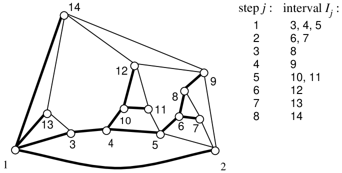
Figure 2: A triconnected plane graph $G$ and a canonical ordering of $G$.

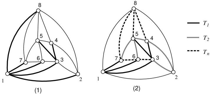
Figure 3: $(1)$ a canonical ordering of a plane triangulation $G$; $(2)$ a realizer of $G$.

Given a canonical ordering of $G$ with its unique partition $I_{1},I_{2},\ldots,I_{K}$, $G=G_{n}$ is obtainable from $G_{2}=\{(v_{1},v_{2})\}$ in $K$ steps, one for each $I_{j}$. Step $j$ obtains $G_{k+q}$ from $G_{k-1}$ by adding the path $v_{k},v_{k+1},\ldots,v_{k+q}$ and its incident edges to $G_{k-1}$. This process is called the construction algorithm for $G$ corresponding to the ordering.

For the given ordering, the canonical spanning tree $T$ of $G$ rooted at $v_{1}$ is the one formed by the edge $(v_{1},v_{2})$ together with the paths $C_{j}$ and the edges $(v_{\ell},v_{k})$ over all $I_{j}$. In Figures 2 and 3(1), $T$ is indicated by thick lines.

Lemma 2.4

1. For every edge $(v_{i},v_{i^{\prime}})$ in $G-T$, $v_{i}$ and $v_{i^{\prime}}$ are not related in $T$.

2. For each node $v_{i}$, the edges incident to $v_{i}$ in $G$ form the following pattern around $v_{i}$ in the counterclockwise order: an edge to its parent in $T$; followed by a block of nontree edges to lower-numbered nodes; followed by a block of tree edges to its children in $T$; followed by a block of nontree edges to higher-numbered nodes, where a block may be empty.

Proof.

Statement 1. Suppose that $(v_{i},v_{i^{\prime}})$ is added at step $j$ of the construction algorithm for $G$. Either $v_{i}$ or $v_{i^{\prime}}$ is on the path $v_{k},v_{k+1},\ldots,v_{k+q}$ and the other is to the right of $v_{\ell}$ on $H_{k-1}$. Hence $v_{i}$ is neither an ancestor nor a descendant of $v_{i^{\prime}}$ in $T$.

Statement 2. Suppose that $v_{i}$ is added at step $j$. The tree edge from $v_{i}$ to its parent, i.e., $v_{\ell}$ or $v_{i-1}$, and all the nontree edges between $v_{i}$ and its lower-numbered neighbors are added during this step; if $i<k+q$, no such nontree edge exists. All such nontree edges precede other edges incident to $v_{i}$ in the counterclockwise order. Any edge $e=(v_{i},v_{i^{\prime}})$ with $i<i^{\prime}$ is added during step $j^{\prime}$ with $j<j^{\prime}$. Let $I_{j^{\prime}}=[k^{\prime},k^{\prime}+q^{\prime}]$. Thus, $e$ is a tree edge only if $i^{\prime}=k^{\prime}$ and $v_{i}$ is the leftmost neighbor of $v_{i^{\prime}}$ in $H_{i^{\prime}-1}$ for otherwise $e$ would be a nontree edge. The tree edges between $v_{i}$ and its children, which are higher numbered, precede the nontree edges between $v_{i}$ and its higher-numbered neighbors in the counterclockwise order.        

Let $T^{\prime}$ be a tree embedded on the plane. Let $(x,y)$ be an edge of $T^{\prime}$. The counterclockwise preordering of $T^{\prime}$ starting at $x$ and $y$ is defined as follows. We perform a preorder traversal on $T^{\prime}$ starting at $x$ and using $(x,y)$ as the first visited edge. Once a node $v$ is visited via $(w,v)$, the unvisited nodes adjacent to $v$ are visited in the counterclockwise order around $v$ starting from the first edge following $(w,v)$.

Fact 6 (see [14, 9])

For every triconnected plane graph, the counterclockwise preordering of any canonical spanning tree is also a canonical ordering of the graph.

Remark. The canonical ordering in Figure 2 is the counterclockwise preordering of $T$.

Assume that $G$ is a triangulation with exterior nodes $v_{1},v_{2},v_{n}$ in the counterclockwise order. A realizer of $G$ is a partition of the interior edges of $G$ into three trees $T_{1},T_{2},T_{n}$ rooted at $v_{1},v_{2},v_{n}$ respectively with the following properties [24]:

1. All the interior edges incident to $v_{1}$ ($v_{2}$ or $v_{n}$, respectively) belong to $T_{1}$ ($T_{2}$ or $T_{n}$, respectively) and oriented to $v_{1}$ ($v_{2}$ or $v_{n}$, respectively).

2. For each interior node $v$, the edges incident to $v$ form the following pattern around $v$ in the counterclockwise order: an edge in $T_{1}$ leaving $v$; followed by a block of edges in $T_{n}$ entering $v$; an edge in $T_{2}$ leaving $v$; followed by a block of edges in $T_{1}$ entering $v$; an edge in $T_{n}$ leaving $v$; followed by a block of edges in $T_{2}$ entering $v$, where a block may be empty.

Figure 3(2) illustrates a realizer of the plane triangulation of Figure 3(1). The next fact relates a canonical ordering and a realizer via counterclockwise tree preordering.

Fact 7 (see [14, 24])

Let $G$ be a plane triangulation.

1. Let $v_{1},v_{2},\ldots,v_{n}$ be a canonical ordering of $G$. Note that each $I_{j}$ consists of a node $v_{k}$. Orient and partition the interior edges of $G$ into three subsets $T_{1},T_{2},T_{n}$ as follows. For each $v_{k}$ with $k\geq 3$, $(v_{k},v_{\ell})$ is in $T_{1}$ oriented to $v_{\ell}$; $(v_{k},v_{r})$ is in $T_{2}$ oriented to $v_{r}$; the edges $(v_{k},v_{i})$ where $\ell<i<r$ are in $T_{n}$ oriented to $v_{k}$. Then $T_{1},T_{2},T_{n}$ is a realizer of $G$. Consequently, every plane triangulation has a realizer that can be constructed in linear time.

2. For a realizer $T_{1},T_{2},T_{n}$ of $G$, let $T=T_{1}\cup\{(v_{1},v_{2}),(v_{1},v_{n})\}$. Let $v_{1},v_{2},\ldots,v_{n}$ be the counterclockwise preordering of $T$ that starts at $v_{1}$ and uses $(v_{1},v_{2})$ as the first visited edge. Then $v_{1},v_{2},\ldots,v_{n}$ is a canonical ordering of $G$, and $T$ is a canonical spanning tree rooted at $v_{1}$.

In Figure 3(1), the tree $T$ stated in Fact 7(2) is indicated by thick lines, and the canonical ordering shown is the counterclockwise preordering of $T$.

3 Schemes with Query Support

This section presents our coding schemes that support queries. We give a weakly convenient encoding in §3.1. This encoding illustrates the basic techniques applicable to our coding schemes with query support. We then give the schemes for triconnected, triangulated, and general plane graphs in §3.2,  §3.3, and §3.4, respectively. We show how to accommodate self-loops in §3.5.

3.1 Basic Techniques

• Let $G_{s}$ be a simple plane graph with $n$ nodes and $m_{s}$ edges.

• Let $T$ be a spanning tree of $G_{s}$ that satisfies Lemma 2.4. Let $n^{*}$ be the number of leaves in $T$. Let $v_{1},\ldots,v_{n}$ be the counterclockwise preordering of $T$.

• Let $G_{a}$ be a graph obtained from $G_{s}$ by adding multiple edges between adjacent nodes in $G_{s}-T$. Let $m_{a}$ be the number of edges in $G_{a}$, counting multiple edges.

We now give a weakly convenient encoding for $G_{a}$ using parentheses to encode $T$ and brackets to encode the edges in $G_{a}-T$. Initially, let $S=F(T)$. Let ${\mbox{\tt(}_{i}}$ and ${\mbox{\tt)}_{i}}$ be the parenthesis pair corresponding to $v_{i}$ in $S$. We insert into $S$ a pair ${\mbox{\tt[}_{e}}$ and ${\mbox{\tt]}_{e}}$ for each edge $e=(v_{i},v_{j})$ of $G_{a}-T$ with $i<j$ as follows.

• ${\mbox{\tt[}_{e}}$ is placed right after ${\mbox{\tt)}_{i}}$, and

• ${\mbox{\tt]}_{e}}$ is placed right after ${\mbox{\tt(}_{j}}$.

For example, the string $S$ for the graph in Figure 3 is:

(()[[[(](])[[(])[[[)[(]])[(]])[(]]]]))

122 3 4 4 5 5 3 6 6 7 7 8 81

Note that if $v_{i}$ is adjacent to $\ell_{i}$ lower-numbered nodes and $h_{i}$ higher-numbered nodes in $G_{a}-T$, then in $S$ the open parenthesis ${\mbox{\tt(}_{i}}$ is immediately followed by $\ell_{i}$ close brackets, and the close parenthesis ${\mbox{\tt)}_{i}}$ by $h_{i}$ open brackets.

Lemma 3.1

The last parenthesis that precedes an open $($respectively, close$)$ bracket in $S$ is close $($respectively, open$)$.

Proof. Straightforward.        

Let $e=(v_{i},v_{j})$ be an edge of $G_{a}-T$ with $i<j$. By Lemma 2.4(1), $v_{i}$ and $v_{j}$ are not related. By Fact 3(2), ${\mbox{\tt)}_{i}}$ precedes ${\mbox{\tt(}_{j}}$ in $S$. Also, ${\mbox{\tt[}_{e}}$ precedes ${\mbox{\tt]}_{e}}$ in $S$ for every edge $e$ in $G_{a}-T$, counting multiple edges. Note that ${\mbox{\tt[}_{e}}$ and ${\mbox{\tt]}_{e}}$ do not necessarily match each other in $S$. In the next lemma, let $S[p]<S[q]$ denote that $S[p]$ precedes $S[q]$ in $S$, i.e., $p<q$.

Lemma 3.2

Let $e$ and $f$ be two edges in $G_{a}-T$ with no common endpoint. If ${\mbox{\tt[}_{e}}<{\mbox{\tt[}_{f}}$, then either ${\mbox{\tt[}_{e}}<{\mbox{\tt]}_{e}}<{\mbox{\tt[}_{f}}<{\mbox{\tt]}_{f}}$ or ${\mbox{\tt[}_{e}}<{\mbox{\tt[}_{f}}<{\mbox{\tt]}_{f}}<{\mbox{\tt]}_{e}}$.

Proof. Suppose $e=(v_{i},v_{j})$ and $f=(v_{k},v_{h})$, where $i<j$ and $k<{h}$. Assume for a contradiction that ${\mbox{\tt[}_{e}}<{\mbox{\tt[}_{f}}<{\mbox{\tt]}_{e}}<{\mbox{\tt]}_{f}}$. Since $e$ and $f$ have no common endpoint, ${\mbox{\tt)}_{i}}<{\mbox{\tt)}_{k}}<{\mbox{\tt(}_{j}}<{\mbox{\tt(}_{{h}}}$. There are four possible cases:

1. ${\mbox{\tt(}_{k}}<{\mbox{\tt(}_{i}}<{\mbox{\tt)}_{i}}<{\mbox{\tt)}_{k}}<{\mbox{\tt(}_{j}}<{\mbox{\tt(}_{{h}}}<{\mbox{\tt)}_{{h}}}<{\mbox{\tt)}_{j}}$; see Figure 4(1).

2. ${\mbox{\tt(}_{i}}<{\mbox{\tt)}_{i}}<{\mbox{\tt(}_{k}}<{\mbox{\tt)}_{k}}<{\mbox{\tt(}_{j}}<{\mbox{\tt(}_{{h}}}<{\mbox{\tt)}_{{h}}}<{\mbox{\tt)}_{j}}$; see Figure 4(2).

3. ${\mbox{\tt(}_{k}}<{\mbox{\tt(}_{i}}<{\mbox{\tt)}_{i}}<{\mbox{\tt)}_{k}}<{\mbox{\tt(}_{j}}<{\mbox{\tt)}_{j}}<{\mbox{\tt(}_{{h}}}<{\mbox{\tt)}_{{h}}}$; see Figure 4(3).

4. ${\mbox{\tt(}_{i}}<{\mbox{\tt)}_{i}}<{\mbox{\tt(}_{k}}<{\mbox{\tt)}_{k}}<{\mbox{\tt(}_{j}}<{\mbox{\tt)}_{j}}<{\mbox{\tt(}_{{h}}}<{\mbox{\tt)}_{{h}}}$; see Figure 4(4).

In Figure 4, the dark lines are paths in $T$ and the dashed ones are edges in $G_{a}-T$. The relation among these lines follows from Fact 3 and Lemma 2.4(2). In all the cases, $e$ crosses $f$, contradicting the fact that $G_{a}$ is a plane graph.        

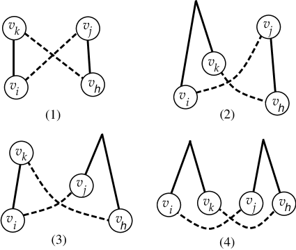
Figure 4: Edge crossing

By Lemma 3.2, ${\mbox{\tt]}_{e}}$ and the bracket that matches ${\mbox{\tt[}_{e}}$ in $S$ are in the same block of brackets. From here onwards, we rename the close brackets by redefining ${\mbox{\tt]}_{e}}$ to be the close bracket that matches ${\mbox{\tt[}_{e}}$ in $S$. Note that Lemma 3.1 still holds for $S$.

Lemma 3.3

$S+\alpha(S)$ is a weakly convenient encoding for $G_{a}$.

Proof. Since $T$ is simple, by Theorem 2.2 $S+\alpha(S)$ is a weakly convenient encoding for $T$. We next show that $S+\alpha(S)$ is also a weakly convenient encoding for $G_{a}-T$. Let $p_{i}$ and $q_{i}$ be the positions of ${\mbox{\tt(}_{i}}$ and ${\mbox{\tt)}_{i}}$ in $S$, respectively.

Case 1: adjacency queries. Suppose $i<j$. Then, $v_{i}$ and $v_{j}$ are adjacent in $G_{a}-T$ if and only if $q_{i}<p<q<{\rm first}_{1}({p_{j}})$, where $(p,q)={\rm enclose}_{2}({{\rm first}_{1}({q_{i}}),p_{j}})$ as shown below.

$$\begin{array}[]{cccccc}{\mbox{\tt)}_{i}}&{\mbox{\tt[}}&&{\mbox{\tt(}_{j}}&{\mbox{\tt]}}\\ \uparrow&\uparrow&\uparrow&\uparrow&\uparrow&\uparrow\\ q_{i}&p&{\rm first}_{1}({q_{i}})&p_{j}&q&{\rm first}_{1}({p_{j}})\end{array}$$

Case 2: neighbor and degree queries. The neighbors and thus the degree of a degree-$d$ node $v_{i}$ in $G_{a}-T$ are obtainable in $O(d)$ time as follows.

For each position $p$ such that $q_{i}<p<{\rm first}_{1}({q_{i}})$, we output $v_{j}$, where $p_{j}={\rm last}_{1}({{\rm match}({p})})$ as shown below. Note that $(v_{i},v_{j})$ is an edge in $G_{a}-T$ with $j>i$.

$$\begin{array}[]{ccccc}{\mbox{\tt)}_{i}}&{\mbox{\tt[}}&&{\mbox{\tt(}_{j}}&{\mbox{\tt]}}\\ \uparrow&\uparrow&\uparrow&\uparrow&\uparrow\\ q_{i}&p&{\rm first}_{1}({q_{i}})&p_{j}&{\rm match}({p})\end{array}$$

For each position $q$ such that $p_{i}<q<{\rm first}_{1}({p_{i}})$, we output $v_{j}$, where $q_{j}={\rm last}_{1}({{\rm match}({q})})$ as shown below. Note that $(v_{i},v_{j})$ is an edge in $G_{a}-T$ with $j<i$.

$$\begin{array}[]{cccccc}{\mbox{\tt)}_{j}}&{\mbox{\tt[}}&{\mbox{\tt(}_{i}}&{\mbox{\tt]}}\\ \uparrow&\uparrow&\uparrow&\uparrow&\uparrow\\ q_{j}&{\rm match}({q})&p_{i}&q&{\rm first}_{1}({p_{i}})\end{array}$$

     

Since $|S|=2n+2(m_{a}-n+1)=2m_{a}+2$ and $S$ uses four symbols, $S$ can be encoded by $4m_{a}+4$ bits. The next lemma improves this bit count.

Lemma 3.4

Let $S^{\prime}$ be a string of $s_{1}$ parentheses and $s_{2}$ brackets that satisfies Lemma 3.1. Then $S^{\prime}$ can be encoded by a string of $2s_{1}+s_{2}+o(s_{1}+s_{2})$ bits, from which each $S^{\prime}[i]$ can be determined in $O(1)$ time.

Proof. Let $S^{\prime}_{1}$ and $S^{\prime}_{2}$ be two binary strings defined as follows, both obtainable in $O(|S^{\prime}|)$ time:

• $S^{\prime}_{1}[i]=1$ if and only if $S^{\prime}[i]$ is a parenthesis for $1\leq i\leq s_{1}+s_{2}$;

• $S^{\prime}_{2}[j]=1$ if and only if the $j$-th parenthesis in $S^{\prime}$ is open for $1\leq j\leq s_{1}$.

Each $S^{\prime}[i]$ can be determined from $S^{\prime}_{1}+S^{\prime}_{2}+\alpha(S^{\prime}_{1})$ in $O(1)$ time as follows. Let $j={\rm rank}({S^{\prime}_{1},i,\mbox{1}})$. If $S^{\prime}_{1}[i]=1$, $S^{\prime}[i]$ is a parenthesis. Whether it is open or close can be determined from $S^{\prime}_{2}[j]$. If $S^{\prime}_{1}[i]=0$, $S^{\prime}[i]$ is a bracket. Whether it is open or close can be determined from $S^{\prime}_{2}[{\rm select}({S^{\prime}_{1},{\rm rank}({S^{\prime}_{1},i,\mbox{1}}),\mbox{1}})]$ by Lemma 3.1.        

The next lemma summarizes the above discussion.

Lemma 3.5

$G_{a}$ has a weakly convenient encoding of $2m_{a}+2n+o(m_{a}+n)$ bits, from which the degree of a node in $G_{a}-T$ is obtainable in $O(1)$ time.

Proof. This lemma follows from Lemmas 3.1, 3.3, and 3.4 and the fact that $S$ contains $2n$ parentheses and $2(m_{a}-n+1)$ brackets.        

3.2 Triconnected Plane Graphs

This section adopts all the notation of §3.1 with the following further definitions.

• Let $G$ be a triconnected plane graph.

• Let $G_{s}$ be the simple version of $G$.

• Let $T$ be a canonical spanning tree of $G_{s}$, which therefore satisfies Lemma 2.4.

Note that $G$ is obtained from $G_{a}$ be adding multiple edges between adjacent nodes in $T$. We next show that the weakly convenient encoding for $G_{a}$ in Lemma 3.5 can be shortened to $2(m_{a}+n-n^{*})+o(n)$ bits. We also give a convenient encoding for $G_{a}$ of $2m_{a}+2n+o(n)$ bits. Then we augment both encodings to accommodate multiple edges in $T$. This gives encodings of $G$.

Let $v_{h}$ be a leaf of $T$ with $2<h<n$. By the definitions of $T$ and a canonical ordering, $v_{h}$ is adjacent to at least one higher-numbered node and at least two distinct lower-numbered nodes in $G_{a}$. By the definition of $T$, the parent of $v_{h}$ in $T$, i.e., the only neighbor of $v_{h}$ in $T$, has a lower number than $v_{h}$. Thus, $v_{h}$ is adjacent to a higher-numbered node and a lower-numbered one in $G_{a}-T$. Thus, ${\mbox{\tt(}_{h}}$ is immediately succeeded by a ], and ${\mbox{\tt)}_{h}}$ by a [. With these observations, we can remove a pair of brackets for every $v_{h}$ from $S$ without losing any information on $G_{a}$ as follows. Let $P$ be the string obtained from $S$ by removing the ] that immediately succeeds ${\mbox{\tt(}_{h}}$ as well as the [ that immediately succeeds ${\mbox{\tt)}_{h}}$ for every $v_{h}$. Let $Q$ be the string obtained from $S$ by removing ${\mbox{\tt(}_{h}}$ and ${\mbox{\tt)}_{h}}$ for every $v_{h}$.

Note that $|P|=|Q|$. Also, $Q[i]$ is obtainable from $P+\alpha(P)$ in $O(1)$ time as follows:

$$Q[i]=\left\{\begin{array}[]{ll}{\mbox{\tt]}}&\mbox{if $P[i]={\mbox{\tt(}}$, $P[{\rm first}_{1}({P,i})]={\mbox{\tt)}}$, and $2<{\rm rank}({P,i,{\mbox{\tt(}}})<n$};\\ {\mbox{\tt[}}&\mbox{if $P[i]={\mbox{\tt)}}$, $P[{\rm last}_{1}({P,i})]={\mbox{\tt(}}$, and $2<{\rm rank}({P,i,{\mbox{\tt(}}})<n$};\\ P[i]&\mbox{otherwise}.\end{array}\right.$$

Lemma 3.6

$P+Q+\alpha(P,Q)$ is a weakly convenient encoding for $G_{a}$, and a convenient encoding for $G_{a}-T$.

Proof. Note that the parentheses in $P$ form $F(T)$. Thus, by Theorem 2.2, it suffices to show that $P+Q+\alpha(P,Q)$ is a convenient encoding for $G_{a}-T$ as follows.

Case 1: adjacency queries. Given $i<j$, let $(p,q)={\rm enclose}_{2}({Q,{\rm first}_{1}({P,q_{i}}),p_{j}-1})$; the $-1$ in the last parameter accounts for the possibility that $Q[p_{j}]$ is a bracket. Note that $v_{i}$ is adjacent to $v_{j}$ if and only if $q_{i}\leq p<q<{\rm first}_{1}({P,p_{j}})$ as shown below. Here, the first inequality accounts for the possibility of $Q[q_{i}]$ being a bracket.

$$\begin{array}[]{ccccccc}P&{\mbox{\tt)}_{i}}&&&{\mbox{\tt(}_{j}}\\ Q&&{\mbox{\tt[}}&&&{\mbox{\tt]}}\\ &\uparrow&\uparrow&\uparrow&\uparrow&\uparrow&\uparrow\\ &q_{i}&p&{\rm first}_{1}({P,q_{i}})&p_{j}&q&{\rm first}_{1}({P,p_{j}})\end{array}$$

Case 2: neighbor queries. The neighbors of $v_{i}$ can be listed as follows.

For every position $p$ with $q_{i}-\delta(Q[q_{i}]={\mbox{\tt[}})<p<{\rm first}_{1}({P,q_{i}})$, we output $v_{j}$, where $p_{j}={\rm last}_{1}({P,{\rm match}({Q,p})+1})$ as shown below. Note that the $+1$ in the last parameter accounts for the possibility of $P[{\rm match}({Q,p})]$ being a parenthesis. Also, $(v_{i},v_{j})$ is an edge in $G_{a}-T$ with $j>i$.

$$\begin{array}[]{ccccccc}P&{\mbox{\tt)}_{i}}&&&{\mbox{\tt(}_{j}}\\ Q&&{\mbox{\tt[}}&&&{\mbox{\tt]}}\\ &\uparrow&\uparrow&\uparrow&\uparrow&\uparrow\\ &q_{i}&p&{\rm first}_{1}({P,q_{i}})&p_{j}&{\rm match}({Q,p})\end{array}$$

For every position $q$ with $p_{i}-\delta(Q[p_{i}]={\mbox{\tt]}})<q<{\rm first}_{1}({P,p_{i}})$, we output $v_{j}$, where $q_{j}={\rm last}_{1}({P,{\rm match}({Q,q})+1})$ as shown below. Note that the $+1$ in the last parameter accounts for the possibility of $P[{\rm match}({Q,q})]$ being a parenthesis. Note that $(v_{i},v_{j})$ is an edge in $G_{a}-T$ with $j<i$.

$$\begin{array}[]{ccccccc}P&{\mbox{\tt)}_{j}}&&{\mbox{\tt(}_{i}}&&\\ Q&&{\mbox{\tt[}}&&{\mbox{\tt]}}&\\ &\uparrow&\uparrow&\uparrow&\uparrow&\uparrow\\ &q_{j}&{\rm match}({Q,q})&p_{i}&q&{\rm first}_{1}({P,p_{i}})\end{array}$$

Case 3: degree queries. The degree of $v_{i}$ in $G_{a}-T$ is ${\rm first}_{1}({P,q_{i}})-q_{i}+\delta(Q[q_{i}]={\mbox{\tt[}})+{\rm first}_{1}({P,p_{i}})-p_{i}+\delta(Q[p_{i}]={\mbox{\tt]}})-2$, obtainable from $P+Q+\alpha(P,Q)$ in $O(1)$ time.        

Lemma 3.7

$G_{a}$ has a weakly convenient encoding of $2m_{a}+2n-2n^{*}+o(m_{a}+n)$ bits, from which the degree of a node in $G_{a}-T$ is obtainable in $O(1)$ time. Moreover, $G_{a}$ has a convenient encoding of $2m_{a}+2n-n^{*}+o(m_{a}+n)$ bits.

Proof. Since each $Q[i]$ is obtainable from $P+\alpha(P)$ in $O(1)$ time, by Lemma 3.6, $P+\alpha(P,Q)$ is also a weakly convenient encoding for $G_{a}$. Since $S$ satisfies Lemma 3.1 and $P$ is obtained from $S$ by removing some brackets, $P$ also satisfies Lemma 3.1. Since $P$ has $2n$ parentheses and $2(m_{a}-(n-1)-n^{*})$ brackets, by Lemma 3.4, $G_{a}$ has a weakly convenient encoding of $2(m_{a}+n-n^{*})+o(m_{a}+n)$ bits. To augment this weakly convenient encoding into a convenient one, note that the degree of $v_{i}$ in $G_{a}-T$ is obtainable in $O(1)$ time from $P+Q+\alpha(P,Q)$. By Theorem 2.3(2), $n^{*}+o(n)$ additional bits suffice for supporting a degree query for $T$ in $O(1)$ time. Thus, $G_{a}$ has a convenient encoding of $2m_{a}+2n-n^{*}+o(m_{a}+n)$ bits.        

The next theorem summarizes the above discussion and extends Lemma 3.7 to accommodate multiple edges in $T$.

Theorem 3.8

Let $G$ be a triconnected plane graph of $n$ nodes and $m$ edges. Let $G_{s}$ be the simple version of $G$ with $m_{s}$ edges. Let $n^{*}$ be the number of leaves in a canonical spanning tree $T$ of $G_{s}$. Then $G$ $($respectively, $G_{s}$$)$ has a convenient encoding of $2m+3n-n^{*}+o(m+n)$ $($respectively, $2m_{s}+2n-n^{*}+o(n)$$)$ bits.

Proof. The statement for $G_{s}$ follows immediately from Lemma 3.7 with $G_{a}=G_{s}$.

To prove the statement for $G$, let $G_{a}$ be the graph obtained from $G_{s}$ by adding the multiple edges of $G$ between adjacent nodes in $G_{s}-T$. By Lemma 3.7, if $G_{a}$ has $m_{a}$ edges, then $G_{a}$ has a weakly convenient encoding of $2(m_{a}+n-n^{*})+o(m_{a}+n)$ bits, from which a degree query for $G_{a}-T$ takes $O(1)$ time. Next, let $T_{b}=G-(G_{a}-T)$. To support degree queries for $T_{b}$, note that $T_{b}$ is a multiple tree of $n$ nodes and $m-m_{a}+n-1$ edges. By Theorem 2.3(1), $2(m-m_{a}+n-1)-n+n^{*}+o(m)$ additional bits suffice for supporting a degree query of $T_{b}$ in $O(1)$ time. Thus, $G$ has a convenient encoding of $2m+3n-n^{*}+o(m)$ bits.        

3.3 Plane Triangulations

Since every plane triangulation is triconnected, all the coding schemes of Theorem 3.8 are applicable to plane triangulations. The next theorem shortens their encodings. The theorem and its proof adopt the notation of §3.1 and §3.2.

Theorem 3.9

Assume that $G$ is a plane triangulation of $n$ nodes and $m$ edges. Let $G_{s}$ be the simple version of $G$ with $m_{s}=3n-6$ edges. Then $G$ $($respectively, $G_{s}$$)$ has a convenient encoding of $2m+2n+o(m+n)$ $($respectively, $2m_{s}+n+o(n)$$)$ bits.

Proof. By the definition of a canonical ordering, every $v_{i}$ with $1<i<n$ is adjacent to a higher-numbered and a lower-numbered node in $G_{s}-T$. Thus when computing the $P$ of §3.2 from $S$, we can also remove the [ right after ${\mbox{\tt)}_{i}}$ even if $v_{i}$ is internal in $T$. Then, the string $Q$ of length $|P|$ is redefined as follows:

$$Q[i]=\left\{\begin{array}[]{ll}{\mbox{\tt]}}&\mbox{if $P[i]={\mbox{\tt(}}$, $P[{\rm first}_{1}({P,i})]={\mbox{\tt)}}$, and $2<{\rm rank}({P,i,{\mbox{\tt(}}})<n$};\\ {\mbox{\tt[}}&\mbox{if $P[i]={\mbox{\tt)}}$ and $1<{\rm rank}({P,i,{\mbox{\tt(}}})<n$};\\ P[i]&\mbox{otherwise}.\end{array}\right.$$

The proof of Lemma 3.6 works identically. Since the count of brackets decreases by $n-n^{*}+O(1)$, each encoding in Theorem 3.8 has $n-n^{*}+O(1)$ fewer bits.        

3.4 General Plane Graphs

This section assumes that if a plane graph has more than one connected component, then no connected component is inside an interior face of another connected component.

Let $\hat{G}_{s}$ be a simple plane graph with $n$ nodes, $\hat{m}_{s}$ edges, and $c$ connected components $\hat{M}_{1},\hat{M}_{2},\ldots,\hat{M}_{c}$. Let $\hat{n}_{j}$ and $\hat{m}_{j}$ be the numbers of nodes and edges in $\hat{M}_{j}$.

For each $\hat{M}_{j}$, we define a graph $M_{j}$ as follows. If $\hat{n}_{j}<3$, let $M_{j}=\hat{M}_{j}$. If $\hat{n}_{j}\geq 3$, let $M_{j}$ be a graph obtained by triangulating $\hat{M}_{j}$. Among the $3\hat{n}_{j}-6$ edges in $M_{j}$, the ones in $\hat{M}_{j}$ are called real, and the others are unreal.

For each $M_{j}$, we define a spanning tree $T_{j}$ as follows. If $\hat{n}_{j}<3$, let $T_{j}$ be an arbitrary rooted spanning tree of $M_{j}$. For $\hat{n}_{j}\geq 3$, recall that by Fact 7(1), $M_{j}$ has a realizer formed by three edge-disjoint trees. Furthermore, three canonical spanning trees $T_{j}^{1},T_{j}^{2},T_{j}^{3}$ of $M_{j}$ are obtainable by adding to each of these three trees two boundary edges of the exterior face of $M_{j}$. Let $T_{j}$ be a tree among $T_{j}^{1},T_{j}^{2},T_{j}^{3}$ with the least number of unreal edges.

Let $T$ be the tree rooted at a new node $v_{0}$ by joining the root of each $T_{j}$ to $v_{0}$ with an unreal edge; note that $T$ is obtainable in $O(n)$ time by Fact 7. Let $m_{u}$ be the number of the unreal edges of $T$; thus, $T$ has $n-m_{u}$ real edges. Let $v_{0},v_{1},v_{2},\ldots,v_{n}$ be a counterclockwise preordering of $T$. Let $d_{i}$ be the degree of $v_{i}$ in $T$. Let $N_{k}$ be the number of nodes of degree more than $k$ in $T$.

Let $G_{s}$ be the simple graph composed of the edges in $\hat{G}_{s}$ and the unreal edges in $T$. A node of $G_{s}$ is real if its incidental edge to its parent in $T$ is real; note that each child of $v_{0}$ in $T$ is unreal.

Let $E_{a}$ be a set of $\ell_{a}$ multiple edges between adjacent nodes in $G_{s}-T$. Let $G_{a}=G_{s}\cup E_{a}$ and $\hat{G}_{a}=\hat{G}_{s}\cup E_{a}$. Let $m_{a}$ and $\hat{m}_{a}$ be the numbers of edges in $G_{a}$ and $\hat{G}_{a}$, respectively; i.e., $m_{a}=m_{s}+\ell_{a}$ and $\hat{m}_{a}=\hat{m}_{s}+\ell_{a}$.

Lemma 3.10

1. $m_{u}\leq n-\frac{1}{3}\hat{m}_{s}.$

2. $m_{u}-c\leq\frac{2}{3}n.$

3. $N_{k}\leq\frac{n}{k}.$

Proof.

Statement 1. Let $u_{j}$ be the number of unreal edges of $T_{j}$. Clearly $m_{u}=c+u_{1}+u_{2}+\cdots+u_{c}$. Since $\hat{m}_{s}=\hat{m}_{1}+\hat{m}_{2}+\cdots+\hat{m}_{c}$, it suffices to prove the claim that $u_{j}\leq\hat{n}_{j}-\frac{1}{3}\hat{m}_{j}-1$ for every $j=1,2,\ldots,c$. For $\hat{n}_{j}\leq 2$, the claim holds trivially. Now suppose $\hat{n}_{j}\geq 3$. For $t=1,2,3$, let $r_{t}$ and $u_{t}$ be the numbers of real and unreal edges in $T_{j}^{t}$, respectively. Since the three trees in a realizer of $M_{j}$ are edge disjoint, $r_{1}+r_{2}+r_{3}+u_{1}+u_{2}+u_{3}-6=3\hat{n}_{j}-9$. Since $r_{1}+r_{2}+r_{3}\geq\hat{m}_{j}$ and $u_{1}+u_{2}+u_{3}\geq 3u_{j}$, the claim holds.

Statement 2.

$$m_{u}-c=\sum_{1\leq j\leq c}u_{j}\leq\sum_{1\leq j\leq c}(\hat{n}_{j}-\frac{1}{3}\hat{m}_{j}-1)\leq\sum_{1\leq j\leq c}(\hat{n}_{j}-\frac{1}{3}(\hat{n}_{j}-1)-1)\leq\frac{2}{3}n.$$

Statement 3. Let $n_{i}$ be the number of nodes of degree $i$ in $T$. Since $T$ is a tree of $n+1$ nodes, we have

$$2n = \sum_{i\geq 1}i\cdot n_{i}\geq n^{*}+n_{2}+\cdots+n_{k}+(k+1)\cdot N_{k};$$

$$n+1 = n^{*}+n_{2}+\cdots+n_{k}+N_{k}.$$

$N_{k}\leq\frac{n}{k}$ follows immediately.        

Lemma 3.11

1. $\hat{G}_{a}$ has a weakly convenient encoding of $2\hat{m}_{a}+2m_{u}+3n+o(\hat{m}_{a}+n)$ bits, from which the degree of a node in $\hat{G}_{a}-T$ is obtainable in $O(1)$ time.

2. $\hat{G}_{a}$ has a convenient encoding of $2\hat{m}_{a}+m_{u}+(4+\frac{1}{k})n+o(\hat{m}_{a}+n)$ bits, for any positive constant $k$.

Proof.

Statement 1. Since each $T_{j}$ is a spanning tree of $M_{j}$ that satisfies Lemma 2.4, $T$ is also a spanning tree of $G_{s}$ that satisfies Lemma 2.4. Then, by Lemma 3.5, $G_{a}$ has a weakly convenient encoding of $2m_{a}+2n+o(m_{a}+n)$ bits, from which the degree of a node in $G_{a}-T$ is obtainable in $O(1)$ time. We next extend this encoding to a desired weakly convenient encoding $X$ for $\hat{G}_{a}$. Since $\hat{G}_{a}-T=G_{a}-T$, it suffices to add an $n$-bit binary string $R$ such that $R[i]=1$ if and only if $v_{i}$ is real. Since $m_{a}=\hat{m}_{a}+m_{u}$, the statement follows.

Statement 2. To augment the above encoding $X$ into a convenient one for $\hat{G}_{a}$, it suffices to support in $O(1)$ time a query on the number $r_{i}$ of real children of $v_{i}$ in $T$. Fix an integer $k$. Let $D$ be a binary string that contains $N_{k}$ copies of $1$. If $v_{i}$ is the $h_{i}$-th node in $v_{1},\ldots,v_{n}$ of degree more than $k$ in $T$, we put $r_{i}$ copies of $0$ right after the $h_{i}$-th $1$ in $D$. The length of $D$ is at most $N_{k}+n-m_{u}$. Since $k=O(1)$, by the definition of a weakly convenient encoding, it takes $O(1)$ time to determine whether $d_{i}>k$ from $X$. If $d_{i}\leq k$, $d_{i}$ and thus the number of real neighbors of $v_{i}$ in $T$ can be computed in $O(1)$ time from $X$. If $d_{i}>k$, the number of real neighbors of $v_{i}$ in $T$ is ${\rm select}({D,h_{i}+1,\mbox{1}})-{\rm select}({D,h_{i},\mbox{1}})-1+R[i]$. To compute $h_{i}$ in $O(1)$ time, let $Y$ be an $n$-bit binary string such that $Y[i]=1$ if and only if $d_{i}>k$. Clearly if $d_{i}>k$, then $h_{i}={\rm rank}({Y,i,\mbox{1}})$, computable in $O(1)$ time from $Y+\alpha(Y)$. Since each $Y[i]$ can be determined in $O(1)$ time from $X$, $Y$ need not be stored in our encoding. In summary, $X+D+\alpha(D,Y)$ is a convenient encoding for $\hat{G}_{a}$, which can be coded in $2\hat{m}_{a}+m_{u}+4n+N_{k}+o(\hat{m}_{a}+n)$ bits. The statement follows immediately from Lemma 3.10(3).        

The next theorem summarizes the above discussion and extends Lemma 3.11 to accommodate multiple edges in $T$.

Theorem 3.12

Let $\hat{G}$ be a plane graph of $n$ nodes and $\hat{m}$ edges. Assume that $\hat{G}_{s}$ is the simple version of $\hat{G}$.

1. $\hat{G}$ $($respectively, $\hat{G}_{s}$$)$ has a weakly convenient encoding of bit count $2\hat{m}+\frac{14}{3}n+o(\hat{m}+n)$ $($respectively, $\frac{4}{3}\hat{m}_{s}+5n+o(n)$$)$.

2. $\hat{G}$ $($respectively, $\hat{G}_{s}$$)$ has a convenient encoding of $2\hat{m}+{(5+\frac{1}{k})}n+o(\hat{m}+n)$ $($respectively, $\frac{5}{3}\hat{m}_{s}+{(5+\frac{1}{k})}n+o(n)$$)$ bits, for any positive constant $k$.

Proof. The statements for $\hat{G}_{s}$ follow immediately from Lemmas 3.10(1) and 3.11 with $\hat{G}_{a}=\hat{G}_{s}$. To prove the statements for $\hat{G}$, we first choose $E_{a}$ to be the set of multiple edges such that $(G_{s}-T)\cup E_{a}$ is composed of the multiple edges of $\hat{G}$ between adjacent nodes in $G_{s}-T$. Also, let $E_{b}=\hat{G}-\hat{G}_{a}$; let $\ell_{b}$ be the number of edges in $E_{b}$.

Statement 1. Continuing the proof of Lemma 3.11(1), we augment the weakly convenient encoding $X$ for $\hat{G}_{a}$ into one for $\hat{G}$. We support in $O(1)$ time a query for the number $a_{i}$ of multiple edges of $\hat{G}$ between $v_{i}$ and its parent in $T$ as follows.

Initially, $L_{0}$ is $n-c$ copies of $1$, one for each node that is not in the first two levels of $T$; recall that all nodes in the first two levels of $T$ are unreal. For $1\leq i\leq n$, suppose that $v_{i}$ is the $g_{i}$-th node in $v_{1},\ldots,v_{n}$ that is not in the first two levels of $T$. We put $a_{i}$ copies of $0$ right after the $g_{i}$-th $1$ in $L_{0}$. Since $\hat{G}$ has $n+\ell_{b}-m_{u}$ edges between adjacent nodes in $T$, $L_{0}$ has $2n-c+\ell_{b}-m_{u}$ bits.

Let $L$ be an $n$-bit binary string such that for $1\leq i\leq n$, $L[i]=1$ if and only if $v_{i}$ is not in the first two levels of $T$. Clearly if $L[i]=1$, then $g_{i}={\rm rank}({L,i,1})$. Since $L[i]$ is obtainable from $X$ in $O(1)$ time, $a_{i}$ is obtainable in $O(1)$ time from $X+L_{0}+\alpha(L_{0},L)$. Moreover, since $R[i]=1$ if and only $a_{i}\geq 1$, $R$ can be removed from $X$. Thus, $\hat{G}$ has a weakly convenient encoding $\hat{X}$ of $2\hat{m}_{a}+m_{u}+4n-c+\ell_{b}+o(\hat{m}_{a}+n)$ bits. The statement follows from Lemma 3.10(2) and the fact that $\hat{m}=\hat{m}_{a}+\ell_{b}$.

Statement 2. We now augment the above encoding $\hat{X}$ into a convenient one for $\hat{G}$. It suffices to support in $O(1)$ time a query on the number $r_{i}$ of the real multiple edges $\hat{G}$ between $v_{i}$ and its children in $T$. Initially, $D$ is $N_{k}$ copies of $1$. Suppose that $v_{i}$ is the $h_{i}$-th node in $v_{1},\ldots,v_{n}$ of degree more than $k$ in $T$. We put $r_{i}$ copies of $0$ right after the $h_{i}$-th $1$ in $D$. As in the proof of Lemma 3.11(2), $h_{i}$ is obtainable from $Y+\alpha(Y)$ in $O(1)$ time, where $Y$ is not stored in the encoding. If $d_{i}>k$, $r_{i}$ is computable as ${\rm select}({D,h_{i}+1,\mbox{1}})-{\rm select}({D,h_{i},\mbox{1}})-1$ in $O(1)$ time. If $d_{i}\leq k$, $r_{i}$ is computable in $O(k)$ time from $\hat{X}$. $D$ has at most $N_{k}+n+\ell_{b}-m_{u}$ bits. Hence $G$ has a convenient encoding $\hat{X}+D+\alpha(D,Y)$ of $2\hat{m}_{a}+5n+2\ell_{b}+N_{k}-c+o(\hat{m}_{a}+\ell_{b}+n)$ bits. Then, this statement follows from Lemma 3.10(3) and the fact $\hat{m}=\hat{m}_{a}+\ell_{b}$.        

3.5 Graphs with Self-loops

Remark. The encodings of Theorems 3.8, 3.9, and 3.12 assume that $G$ has no self-loops. To facilitate the coding of self-loops, we assume that the self-loops incident to a node in a plane graph are recorded at that node by their number. Then, to augment each cited encoding to accommodate self-loops, we only need to add $1$ to the coefficient of the term $n$ in the bit count as follows. Initially, $Z$ is $n$ copies of $1$. Then, for $1\leq i\leq n$, we put $z_{i}$ copies of $0$ right after the $i$-th $1$ in $Z$, where $z_{i}$ is the number of self-loops incident to $v_{i}$. We augment the encoding in question with $Z$ by means of Fact 1. Since the bit count of $Z$ is $n$ plus the number of self-loops, our claims follows from the fact that the coefficient of the term $m$ in the bit count in question is at least one.

4 More Compact Schemes

For applications that require no query support, we obtain more compact encodings for triconnected plane graphs in this section. All graphs in this section are simple.

Let $G$ be a triconnected plane graph with $n>3$ nodes. Let $T$ be a canonical spanning tree of $G$. Let $v_{1},\ldots,v_{n}$ be the counterclockwise preordering of $T$, which by Fact 6 is also a canonical ordering of $G$.

Let $I_{1},\ldots,I_{K}$ be the interval partition for the ordering $v_{1},\ldots,v_{n}$. Recall that the construction algorithm of §2.4 builds $G$ from a single edge $(v_{1},v_{2})$ through a sequence of $K$ steps. The $j$-th step corresponds to the interval $I_{j}=[k,k+q]$. There are two cases, which are used throughout this section.

Case 1: $q=0$, and a single node $v_{k}$ is added.

Case 2: $q>0$, and a chain of $q+1$ nodes $v_{k},\ldots,v_{k+q}$ is added.

The last node added during a step is called type a; the other nodes are type b. Thus for a Case 1 step, $v_{k}$ is type a. For a Case 2 step, $v_{k},v_{k+1},\ldots,v_{k+q-1}$ are type b, and the node $v_{k+q}$ is type a. To define further terms, let $c_{1}=v_{1},c_{2},\ldots,c_{t}=v_{2}$ be the nodes of $H_{k-1}$ ordered consecutively along $H_{k-1}$ from left to right above the edge $(v_{1},v_{2})$.

Case 1. Let $c_{\ell}$ and $c_{r}$, where $1\leq\ell<r\leq t$, be the leftmost and rightmost neighbors of $v_{k}$ in $H_{k-1}$, respectively. The edge $(c_{r},v_{k})$ is called external. The edges $(c_{i},v_{k})$ where $\ell<i<r$, if present, are internal. Note that $(c_{\ell},v_{k})$ is in $T$.

Case 2. Let $c_{\ell}$ and $c_{r}$, where $1\leq\ell<r\leq t$, be the neighbors of $v_{k}$ and $v_{k+q}$ in $H_{k-1}$, respectively. The edge $(c_{r},v_{k})$ is called external. Observe that the edges $(c_{\ell},v_{k}),(v_{k},v_{k+1}),\ldots$, $(v_{k+q-1},v_{k+q})$ are in $T$.

For each $v_{h}$, where $1\leq h\leq n-1$, let $B(v_{h})$ denote the edge set $\{(v_{h},v_{j})~{}|~{}h<j\}$. By the definition of a canonical ordering and Lemma 2.4, the edges in $B(v_{h})$ form the following pattern around $v_{h}$ in the counterclockwise order: a block (maybe empty) of tree edges; followed by at most one internal edge; followed by a block (maybe empty) of external edges. Note that $B(v_{1}),B(v_{2}),\ldots,B(v_{n-1})$ form a partition of the edges of $G$. Also, $B(v_{h})$ is not empty since by the definition of a canonical ordering, every $v_{h}$ is adjacent to some $v_{j}$ with $h<j$.

Lemma 4.1

Given $B(v_{h})$ for $1\leq h\leq n-1$ and the type of $v_{h}$ for $3\leq h\leq n$, we can uniquely reconstruct $G$.

Proof. We first draw $(v_{1},v_{2})$ and then perform the following $K$ steps. Step $j$ processes $I_{j}=[k,k+q]$. Before this step, $G_{k-1}$ and $H_{k-1}$ have been built. Let $c_{1}=v_{1},c_{2},\ldots,c_{t}=v_{2}$ be the nodes on $H_{k-1}$ from left to right. We know the numbers of remaining tree and external edges at each $c_{i}$, i.e., those in $B(c_{i})$ not yet added to $G$. We next find the leftmost neighbor $c_{\ell}$ and the rightmost neighbor $c_{r}$ of the nodes added during this step. Note that $(c_{\ell},v_{k})$ is in $T$. Since $v_{1},\ldots,v_{n}$ is the counterclockwise preordering of $T$, $c_{\ell}$ is the rightmost node with a remaining tree edge; $c_{r}$ is the leftmost node to the right of $c_{\ell}$ with a remaining external edge. There are two cases:

If $v_{k}$ is type a, then this is a Case 1 step and $v_{k}$ is the single node added during this step. We add $(c_{\ell},v_{k})$ and $(c_{r},v_{k})$. For each $c_{i}$ with $\ell<i<r$, if $B(c_{i})$ contains an internal edge, we also add $(c_{i},v_{k})$.

If $v_{k}$ is type b, then this is a Case 2 step. Let $q$ be the integer such that $v_{k},v_{k+1},\ldots,$ $v_{k+q-1}$ are type b and $v_{k+q}$ is type a. The chain $v_{k},\ldots,v_{k+q}$ is added between $c_{\ell}$ and $c_{r}$.

Finally, the number of remaining tree (respectively, external) edges at $c_{\ell}$ (respectively, $c_{r}$) decreases by 1. The numbers of tree, internal, and external edges remaining at each $v_{i}$ for $k\leq i\leq k+q$ are set to those of all tree, internal, and external edges in $B(v_{i})$. This finishes the $j$-th step. When the $K$-th step ends, we have $G$.        

By Lemma 4.1, we can encode $G$ by encoding the types of all $v_{h}$ and $B(v_{h})$ for $1\leq h\leq n-1$ using two strings $S_{1}$ and $S_{2}$. $S_{1}$ is a binary string containing one bit for each $v_{h}$, indicating the type of $v_{h}$. $S_{2}$ encodes the sets $B(v_{h})$ using three symbols $0,1,*$. The code for $B(v_{h})$ is a block of 0’s, followed by a block of 1’s, followed by a block of $*$’s. The number of 0’s (respectively, 1’s and $*$’s) in the first (respectively, second and third) block is that of the tree (respectively, external and internal) edges in $B(v_{h})$. However, since these three numbers can be zero, we need a fourth symbol to separate the codes for $B(v_{h})$. Now if we use two bits to encode each of the 4 symbols used in $S_{2}$, then $S_{2}$ has a longer binary encoding than desired. We next present a shorter encoding by eliminating the symbol used to separate the codes for $B(v_{h})$.

The type of $B(v_{h})$ is defined to be a combination of symbols $T,X$ and $I$, which denote the existences of tree, external or internal edges in $B(v_{h})$, respectively. For example, if $B(v_{h})$ is type $TI$, then it has at least one tree edge, exactly one internal edge, and no external edge; recall that each $B(v_{h})$ has at most one internal edge. Moreover, for all $v_{h}$ of type a, if $B(v_{h})$ has no tree edge, then we call $v_{h}$ type a1; otherwise, $v_{h}$ is type a2. For $v_{h}$ of type b, since $v_{h}$ is added in a Case 2 step and is not the last node added, $B(v_{h})$ has at least one tree edge and thus no similar typing is needed.

Our encoding of $G$ uses two strings $S_{1}$ and $S_{2}$. $S_{1}$ has length $n$. For $1\leq h\leq n$, $S_{1}[h]$ indicates whether $v_{h}$ is type a1, a2, or b, which is recorded by symbols $0,1$, or $*$, respectively. For convenience, let $v_{1}$ be type a2 and $v_{2}$ be type a1. $S_{2}$ uses the same three symbols to encode $B(v_{h})$ for $1\leq h\leq n-1$. $B(v_{h})$ is specified by a codeword ${\rm code}[v_{h}]$ defined in Figure 5. $S_{2}$ is the concatenation of the codewords ${\rm code}[v_{h}]$.

type of $v_{h}$	type of $B(v_{h})$	${\rm code}[v_{h}]$
a1	$XI$	$\underbrace{1^{\beta}}_{X}\underbrace{0}_{I}$
	$I$	$\underbrace{0}_{I}$
	$X$	$\underbrace{1^{\beta-1}*}_{X}$
a2 or b	$T$	$\underbrace{0^{\alpha-1}*}_{T}$
	$TXI$	$\underbrace{1^{\alpha}}_{T}\underbrace{0^{\beta}}_{X}\underbrace{*}_{I}$
	$TX$	$\underbrace{1^{\alpha-1}0}_{T}\underbrace{0^{\beta-1}1}_{X}$
	$TI$	$\underbrace{1^{\alpha}}_{T}\underbrace{*}_{I}$

Figure 5: This code book gives ${\rm code}[v_{h}]$. The length of ${\rm code}[v_{h}]$ is the number of edges in $B(v_{h})$. The numbers of the tree and external edges in $B(v_{h})$ are denoted by $\alpha$ and $\beta$, respectively. Recall that $B(v_{h})$ contain either 0 or 1 internal edge. The notation $z^{t}$ denotes a string of $t$ copies of symbol $z$. A symbol $T$, $X$, or $I$ under ${\rm code}[v_{h}]$ denotes the portion in ${\rm code}[v_{h}]$ corresponding to the tree, external, or internal edges, respectively.

Lemma 4.2

For $1\leq h\leq n-1$, the sets $B(v_{h})$ and the types of all $v_{h}$ can be uniquely determined from $S_{1}$ and $S_{2}$.

Proof. We can look up the type of $v_{h}$ in $S_{1}$. To recover $B(v_{h})$, we perform the following $n-1$ steps. Before step $h$, we know the start index of ${\rm code}[v_{h}]$ in $S_{2}$. With the cases below, step $h$ finds the numbers of tree, external, and internal edges in $B(v_{h})$ as well as the length of ${\rm code}[v_{h}]$, which tells us the start index of ${\rm code}[v_{h+1}]$ in $S_{2}$.

Case A: $v_{h}$ is type a1. There are three subcases.

Case A1: ${\rm code}[v_{h}]$ starts with 0. Then $B(v_{h})$ is type $I$ and contains only one internal edge. Also, ${\rm code}[v_{h}]$ has length 1.

Case A2: ${\rm code}[v_{h}]$ starts with $*$. Then $B(v_{h})$ is type $X$ with $\beta=1$ external edge. Also, ${\rm code}[v_{h}]$ has length 1.

Case A3: ${\rm code}[v_{h}]$ starts with 1. Let $\Theta=1^{\gamma}$ be the maximal block of 1’s in $S_{2}$ at the start of ${\rm code}[v_{h}]$. Then, ${\rm code}[v_{h}]$ has length $\gamma+1$. Let $x$ be the symbol after $\Theta$ in $S_{2}$. There are two further subcases.

If $x=*$, $B(v_{h})$ is type $X$ and has $\beta=\gamma+1$ external edges.

If $x=0$, $B(v_{h})$ is type $XI$ and has $\beta=\gamma$ external edges and one internal edge.

Case B: $v_{h}$ is type a2 or b. Then $B(v_{h})$ contains at least one tree edge. There are three subcases.

Case B1: ${\rm code}[v_{h}]$ starts with $*$. Then $B(v_{h})$ is type $T$ and contains $\alpha=1$ tree edge. Also, ${\rm code}[v_{h}]$ has length 1.

Case B2: ${\rm code}[v_{h}]$ starts with 0. Let $\Theta=0^{\gamma}$ be the maximal block of 0’s in $S_{2}$ at the start of ${\rm code}[v_{h}]$. Then ${\rm code}[v_{h}]$ has length $\gamma+1$. Let $x$ be the symbol after $\Theta$ in $S_{2}$. There are two further subcases:

If $x=*$, then $B(v_{h})$ is type $T$ and has $\alpha=\gamma+1$ tree edges.

If $x=1$, then $B(v_{h})$ is type $TX$ and has 1 tree edge and $\beta=\gamma$ external edges.

Case B3: ${\rm code}[v_{h}]$ starts with 1. Let $\Theta=1^{\gamma}$ be the maximal block of 1’s in $S_{2}$ at the start of ${\rm code}[v_{h}]$. There are three further subcases:

If $*$ follows $\Theta$ in $S_{2}$, then $B(v_{h})$ is type $TI$ and has $\alpha=\gamma$ tree edges and one internal edge. Also, ${\rm code}[v_{h}]$ has length $\gamma+1$.

If $0^{\delta}*$ follows $\Theta$ in $S_{2}$, then $B(v_{h})$ is type $TXI$ and has $\alpha=\gamma$ tree edges, $\beta=\delta$ external edges, and one internal edge. Also, ${\rm code}[v_{h}]$ has length $\gamma+\delta+1$.

If $0^{\delta}1$ follows $\Theta$ in $S_{2}$, then $B(v_{h})$ is type $TX$ and has $\alpha=\gamma+1$ tree edges and $\beta=\delta$ external edges. Also, ${\rm code}[v_{h}]$ has length $\gamma+\delta+1$.

This completes the description of the $h$-th step. In any case above, we can determine the length of ${\rm code}[v_{h}]$ and recover $B(v_{h})$.        

The next theorem summarizes the above discussion.

Theorem 4.3

Let $G$ be a simple triconnected plane graph with $n>3$ nodes, $m$ edges, and $f$ faces.

1. $G$ can be encoded using at most $\log 3{\cdot}(n+m)+1$ bits.

2. $G$ can be encoded using at most $\log 3{\cdot}(\min\{n,f\}+m)+2\leq\frac{3\log 3}{2}m+4$ bits.

Remark. The decoding procedure assumes that the encoding of $G$ is given together with $n$ or $f$ as appropriate, which can be appended to $S$ by means of Fact 1.

Proof.

Statement 1. In the above discussion, $S_{1}$ has length $n$, and $S_{2}$ has length $m$. The encoding $S$ of $G$ is the concatenation of $S_{1}$ and $S_{2}$. Treated as an integer of base 3, $S$ uses at most $\log 3{\cdot}(n+m)+1$ bits.

Statement 2. Let $G^{*}$ be the dual of $G$. $G^{*}$ has $f$ nodes, $m$ edges and $n$ faces. Since $G$ is triconnected, $G^{*}$ is also triconnected. Furthermore, since $n>3$, $f>3$ and $G^{*}$ has no self-loop or multiple edge. Thus, we can use Statement 1 to encode $G^{*}$ with at most $\log 3{\cdot}(f+m)+1$ bits. Since $G$ can be uniquely determined from $G^{*}$, to encode $G$, it suffices to encode $G^{*}$. To shorten $S$, if $n\leq f$, we encode $G$ using at most $\log 3{\cdot}(n+m)+1$ bits; otherwise, we encode $G^{*}$ using at most $\log 3{\cdot}(f+m)+1$ bits. This new encoding uses at most $\log 3{\cdot}(\min\{n,f\}+m)+1$ bits. Since $\min\{n,f\}\leq\frac{n+f}{2}=0.5m+1$, the bit count is at most $\log 3{\cdot}(1.5m)+3$. For the sake of decoding, we use one extra bit to denote whether we encode $G$ or $G^{*}$.

References

- [1] A. V. Aho, J. E. Hopcroft, and J. D. Ullman, The Design and Analysis of Computer Algorithms, Addison-Wesley, Reading, MA, 1974.
- [2] T. C. Bell, J. G. Cleary, and I. H. Witten, Text Compression, Prentice-Hall, Englewood Cliffs, NJ, 1990.
- [3] C. Berge, Graphs, North-Holland, New York, NY, second revised ed., 1985.
- [4] D. R. Clark, Compact Pat Trees, PhD thesis, University of Waterloo, 1996.
- [5] H. de Fraysseix, J. Pach, and R. Pollack, How to draw a planar graph on a grid, Combinatorica, 10 (1990), pp. 41–51.
- [6] P. Elias, Universal codeword sets and representations of the integers, IEEE Transactions on Information Theory, IT-21 (1975), pp. 194–203.
- [7] H. Galperin and A. Wigderson, Succinct representations of graphs, Information and Control, 56 (1983), pp. 183–198.
- [8] M. Grötschel, L. Lovász, and A. Schrijver, Geometric Algorithms and Combinatorial Optimization, Springer-Verlag, New York, NY, 1988.
- [9] X. He, M. Y. Kao, and H. I. Lu, Linear-time succinct encodings of planar graphs via canonical orderings, SIAM Journal on Discrete Mathematics, (1999). To appear.
- [10] A. Itai and M. Rodeh, Representation of graphs, Acta Informatica, 17 (1982), pp. 215–219.
- [11] G. Jacobson, Space-efficient static trees and graphs, in Proceedings of the 30th Annual IEEE Symposium on Foundations of Computer Science, 1989, pp. 549–554.
- [12] S. Kannan, M. Naor, and S. Rudich, Implicit representation of graphs, SIAM Journal on Discrete Mathematics, 5 (1992), pp. 596–603.
- [13] G. Kant, Drawing planar graphs using the -ordering, in Proceedings of the 33rd Annual IEEE Symposium on Foundations of Computer Science, 1992, pp. 101–110.
- [14] , Algorithms for Drawing Planar Graphs, PhD thesis, University of Utrecht, 1993.
- [15] G. Kant and X. He, Regular edge labeling of 4-connected plane graphs and its applications in graph drawing problems, Theoretical Computer Science, 172 (1997), pp. 175–193.
- [16] M. Y. Kao, M. Fürer, X. He, and B. Raghavachari, Optimal parallel algorithms for straight-line grid embeddings of planar graphs, SIAM Journal on Discrete Mathematics, 7 (1994), pp. 632–646.
- [17] M. Y. Kao, N. Occhiogrosso, and S. H. Teng, Simple and efficient compression schemes for dense and complement graphs, Journal of Combinatorial Optimization, 2 (1999), pp. 351–359.
- [18] K. Keeler and J. Westbrook, Short encodings of planar graphs and maps, Discrete Applied Mathematics, 58 (1995), pp. 239–252.
- [19] J. I. Munro, Tables, in Lecture Notes in Computer Science 1180: Proceedings of the 16th Conference on Foundations of Software Technology and Theoretical Computer Science, Springer-Verlag, New York, NY, 1996, pp. 37–42.
- [20] J. I. Munro and V. Raman, Succinct representation of balanced parentheses, static trees and planar graphs, in Proceedings of the 38th Annual IEEE Symposium on Foundations of Computer Science, 1997, pp. 118–126.
- [21] M. Naor, Succinct representations of general unlabeled graphs, Discrete Applied Mathematics, 28 (1990), pp. 303–307.
- [22] C. H. Papadimitriou and M. Yannakakis, A note on succinct representations of graphs, Information and Control, 71 (1986), pp. 181–185.
- [23] R. C. Read, A new method for drawing a planar graph given the cyclic order of the edges at each vertex, Congressus Numerantium, 56 (1987), pp. 31–44.
- [24] W. Schnyder, Embedding planar graphs on the grid, in Proceedings of the 1st Annual ACM-SIAM Symposium on Discrete Algorithms, 1990, pp. 138–148.
- [25] G. Turán, On the succinct representation of graphs, Discrete Applied Mathematics, 8 (1984), pp. 289–294.
- [26] W. T. Tutte, A census of planar triangulations, Canadian Journal of Mathematics, 14 (1962), pp. 21–38.