Benchmarking Optimization Software with Performance Profiles

Abstract

We propose performance profiles — distribution functions for a performance metric — as a tool for benchmarking and comparing optimization software. We show that performance profiles combine the best features of other tools for performance evaluation.

1 Introduction

The benchmarking of optimization software has recently gained considerable visibility. Hans Mittlemann’s Benchmarks work on a variety of optimization software has frequently uncovered deficiencies in the software and has generally led to software improvements. Although Mittelmann’s efforts have gained the most notice, other researchers have been concerned with the evaluation and performance of optimization codes. As recent examples, we cite HYB00; SCB95a; ASB98; BCGT97; CGT96; HM99; RJV99.

The interpretation and analysis of the data generated by the benchmarking process are the main technical issues addressed in this paper. Most benchmarking efforts involve tables displaying the performance of each solver on each problem for a set of metrics such as CPU time, number of function evaluations, or iteration counts for algorithms where an iteration implies a comparable amount of work. Failure to display such tables for a small test set would be a gross omission, but they tend to be overwhelming for large test sets. In all cases, the interpretation of the results from these tables is often a source of disagreement.

The quantities of data that result from benchmarking with large test sets have spurred researchers to try various tools for analyzing the data. The solver’s average or cumulative total for each performance metric over all problems is sometimes used to evaluate performance HYB00; BCGT97; CGT96. As a result, a small number of the most difficult problems can tend to dominate these results, and researchers must take pains to give additional information. Another drawback is that computing averages or totals for a performance metric necessitates discarding problems for which any solver failed, effectively biasing the results against the most robust solvers. As an alternative to disregarding some of the problems, a penalty value can be assigned for failed solver attempts, but this requires a subjective choice for the penalty. Most researchers choose to report the number of failures only in a footnote or separate table.

To address the shortcomings of the previous approach, some researchers rank the solvers BCGT97; CGT96; SGN91; RJV99. In other words, they count the number of times that a solver comes in $k$th place, usually for $k=1,2,3$. Ranking the solvers’ performance for each problem helps prevent a minority of the problems from unduly influencing the results. Information on the size of the improvement, however, is lost.

Comparing the medians and quartiles of some performance metric (for example, the difference between solver times BCGT97) appears to be a viable way of ensuring that a minority of the problems do not dominate the results, but in our testing we have witnessed large leaps in quartile values of a performance metric, rather than gradual trends. If only quartile data is used, then information on trends occurring between one quartile and the next is lost; and we must assume that the journey from one point to another proceeds at a moderate pace. Also, in the specific case of contrasting the differences between solver times, the comparison fails to provide any information on the relative size of the improvement. A final drawback is that if results are mixed, interpreting quartile data may be no easier than using the raw data; and dealing with comparisons of more than two solvers might become unwieldy.

The idea of comparing solvers by the ratio of one solver’s runtime to the best runtime appears in SCB95a, with solvers rated by the percentage of problems for which a solver’s time is termed very competitive or competitive. The ratio approach avoids most of the difficulties that we have discussed, providing information on the percent improvement and eliminating the negative effects of allowing a small portion of the problems to dominate the conclusions. The main disadvantage of this approach lies in the author’s arbitrary choice of limits to define the borders of very competitive and competitive.

In Section 2, we introduce performance profiles as a tool for evaluating and comparing the performance of optimization software. The performance profile for a solver is the (cumulative) distribution function for a performance metric. In this paper we use the ratio of the computing time of the solver versus the best time of all of the solvers as the performance metric. Section 3 provides an analysis of the test set and solvers used in the benchmark results of Sections 4 and 5. This analysis is necessary to understand the limitations of the benchmarking process.

Sections 4 and 5 demonstrate the use of performance profiles with results EDD00 obtained with version 2.0 of the COPS cops-home test set. We show that performance profiles eliminate the influence of a small number of problems on the benchmarking process and the sensitivity of results associated with the ranking of solvers. Performance profiles provide a means of visualizing the expected performance difference among many solvers, while avoiding arbitrary parameter choices and the need to discard solver failures from the performance data.

We conclude in Section 6 by showing how performance profiles apply to the data Benchmarks of Mittelmann for linear programming solvers. This section provides another case study of the use of performance profiles and also shows that performance profiles can be applied to a wide range of performance data.

2 Performance Evaluation

Benchmark results are generated by running a solver on a set $\cal P$ of problems and recording information of interest such as the number of function evaluations and the computing time. In this section we introduce the notion of a performance profile as a means to evaluate and compare the performance of the set of solvers $\cal S$ on a test set $\cal P$.

We assume that we have $n_{s}$ solvers and $n_{p}$ problems. We are interested in using computing time as a performance measure; although, the ideas below can be used with other measures. For each problem $p$ and solver $s$, we define

$$t_{p,s}=\mbox{computing time required to solve problem $p$ by solver $s$.}$$

If, for example, the number of function evaluations is the performance measure of interest, set $t_{p,s}$ accordingly.

We require a baseline for comparisons. We compare the performance on problem $p$ by solver $s$ with the best performance by any solver on this problem; that is, we use the performance ratio

$$r_{p,s}=\frac{t_{p,s}}{\min\{t_{p,s}:s\in\mbox{$\cal S$}\}}.$$

We assume that a parameter $r_{M}\geq r_{p,s}$ for all $p,s$ is chosen, and $r_{p,s}=r_{M}$ if and only if solver $s$ does not solve problem $p$. We will show that the choice of $r_{M}$ does not affect the performance evaluation.

The performance of solver $s$ on any given problem may be of interest, but we would like to obtain an overall assessment of the performance of the solver. If we define

$$\rho_{s}(\tau)=\frac{1}{n_{p}}\mbox{size}\Bigl{\{}p\in\mbox{$\cal P$}:r_{p,s}\leq\tau\Bigr{\}},$$

then $\rho_{s}(\tau)$ is the probability for solver $s\in\mbox{$\cal S$}$ that a performance ratio $r_{p,s}$ is within a factor $\tau\in\R$ of the best possible ratio. The function $\rho_{s}$ is the (cumulative) distribution function for the performance ratio.

We use the term performance profile for the distribution function of a performance metric. Our claim is that a plot of the performance profile reveals all of the major performance characteristics. In particular, if the set of problems $\cal P$ is suitably large and representative of problems that are likely to occur in applications, then solvers with large probability $\rho_{s}(\tau)$ are to be preferred.

The term performance profile has also been used for a plot of some performance metric versus a problem parameter. For example, Higham (NJH96, pages 296–297) plots the ratio $\gamma/\|A\|_{1}$, where $\gamma$ is the estimate for the $l_{1}$ norm of a matrix $A$ produced by the LAPACK condition number estimator. Note that in Higham’s use of the term performance profile there is no attempt at determining a distribution function.

The performance profile $\rho_{s}:\R\mapsto[0,1]$ for a solver is a nondecreasing, piecewise constant function, continuous from the right at each breakpoint. The value of $\rho_{s}(1)$ is the probability that the solver will win over the rest of the solvers. Thus, if we are interested only in the number of wins, we need only to compare the values of $\rho_{s}(1)$ for all of the solvers.

The definition of the performance profile for large values requires some care. We assume that $r_{p,s}\in[1,r_{M}]$ and that $r_{p,s}=r_{M}$ only when problem $p$ is not solved by solver $s$. As a result of this convention, $\rho_{s}(r_{M})=1$, and

$$\rho_{s}^{*}\equiv\lim_{\tau\to r_{M}^{-}}\rho_{s}(\tau)$$

is the probability that the solver solves a problem. Thus, if we are interested only in solvers with a high probability of success, then we need to compare the values of $\rho_{s}^{*}$ for all solvers and choose the solvers with the largest value. The value of $\rho_{s}^{*}$ can be readily seen in a performance profile because $\rho_{s}$ flatlines for large values of $\tau$; that is, $\rho_{s}(\tau)=\rho_{s}^{*}$ for $\tau\in[r_{S},r_{M})$ for some $r_{S}<r_{M}$.

An important property of performance profiles is that they are insensitive to the results on a small number of problems. This claim is based on the observation that if $\rho_{s}$ and $\hat{\rho}_{s}$ are defined, respectively, by the observed time sets $t_{p,s}$ and $\hat{t}_{p,s}$, where

$$\hat{t}_{p,s}=t_{p,s},\qquad p\in\mbox{$\cal P$}\setminus\{q\},$$

for some problem $q\in\mbox{$\cal P$}$, then $\hat{r}_{p,s}=r_{p,s}$ for $p\in\mbox{$\cal P$}\setminus\{q\}$. Since only the ratio $\hat{r}_{q,s}$ changes for any $s\in\mbox{$\cal S$}$,

$$|\rho_{s}(\tau)-\hat{\rho}_{s}(\tau)|\leq\frac{1}{n_{p}},\qquad\tau\in\R,$$

for $s\in\mbox{$\cal S$}$. Moreover, $\hat{\rho}_{s}(\tau)=\rho_{s}(\tau)$ for $\tau<\min\{r_{q,s},\hat{r}_{q,s}\}$ or $\tau\geq\max\{r_{q,s},\hat{r}_{q,s}\}$. Thus, if $n_{p}$ is reasonably large, then the result on a particular problem $q$ does not greatly affect the performance profiles $\rho_{s}$.

Not only are performance profiles relatively insensitive to changes in results on a small number of problems, they are also largely unaffected by small changes in results over many problems. We demonstrate this property by showing that small changes from $r_{p,s}$ to $\hat{r}_{p,s}$ result in a correspondingly small $L_{1}$ error between $\rho_{s}$ and $\hat{\rho}_{s}$.

Theorem 2.1

Let $r_{i}$ and $\hat{r}_{i}$ for $1\leq i\leq n_{p}$ be performance ratios for some solver, and let $\rho$ and $\hat{\rho}$ be, respectively, the performance profiles defined by these ratios. If

$$|r_{i}-\hat{r}_{i}|\leq\epsilon,\qquad 1\leq i\leq n_{p}$$ (2.1)

for some $\epsilon>0$, then

$$\int_{1}^{\infty}\left|\rho(t)-\hat{\rho}(t)\right|\,dt\leq\epsilon$$

Proof

Since performance profiles do not depend on the ordering of the data, we can assume that $\{r_{i}\}$ is monotonically increasing. We can reorder the sequence $\{\hat{r}_{i}\}$ so that it is also monotonically increasing, and (2.1) still holds. These reorderings guarantee that $\rho(t)=i/n_{p}$ for $t\in[r_{i},r_{i+1})$, with a similar result for $\hat{\rho}$. We now show that for any integer $k$ with $1\leq k\leq n_{p}$,

$$\int_{1}^{s_{k}}\left|\rho(t)-\hat{\rho}(t)\right|\,dt\leq k\left(\frac{\epsilon}{n_{p}}\right),$$ (2.2)

where $s_{k}=\max(r_{k},\hat{r}_{k})$, and

$$|r_{i}-\hat{r}_{i}|\leq\epsilon,\quad 1\leq i\leq k,\quad\mbox{and}\quad\hat{r}_{i}=r_{i},\quad k<i\leq n_{p}.$$ (2.3)

The proof is completed when $k=n_{p}$.

The case $k=1$ follows directly from the definition of a performance profile, so assume that (2.2) holds for any performance data such that (2.3) holds. We now prove that (2.2) holds for $k+1$ by proving that

$$\int_{s_{k}}^{s_{k+1}}\left|\rho(t)-\hat{\rho}(t)\right|\,dt\leq\left(\frac{\epsilon}{n_{p}}\right),\qquad k<n_{p}.$$ (2.4)

Together, (2.2) and (2.4) show that (2.2) holds for $k+1$.

We present the proof for the case when $\hat{r}_{k}\leq r_{k}$. A similar argument can be made for $r_{k}\leq\hat{r}_{k}$. If $\hat{r}_{k}\leq r_{k}$ then $s_{k}=r_{k}$ and $\hat{r}_{k}\leq r_{k}\leq r_{k+1}$. The argument depends on the position of $\hat{r}_{k+1}$ and makes repeated use of the fact that $\rho(t)=k/n_{p}$ for $t\in[r_{k},r_{k+1})$, with a similar result for $\hat{\rho}$.

If $r_{k+1}\leq\hat{r}_{k+1}$ then $\rho(t)=\hat{\rho}(t)$ in $[r_{k},r_{k+1})$. Also note that $\left|\rho(t)-\hat{\rho}(t)\right|=1/n_{p}$ in $[r_{k+1},\hat{r}_{k+1})$. Hence, (2.4) holds with $s_{k+1}=\hat{r}_{k+1}$.

The case where $\hat{r}_{k+1}\leq r_{k+1}$ makes use of the observation that $\hat{r}_{i}=r_{i}\geq r_{k+1}$ for $i>k+1$. If $r_{k}\leq\hat{r}_{k+1}\leq r_{k+1}$, then $\rho(t)=\hat{\rho}(t)$ in $[r_{k},\hat{r}_{k+1})$, and $\left|\rho(t)-\hat{\rho}(t)\right|=1/n_{p}$ in $[\hat{r}_{k+1},r_{k+1})$. Hence, (2.4) holds. On the other hand, if $\hat{r}_{k}\leq\hat{r}_{k+1}\leq r_{k}$, then we only need to note that $\left|\rho(t)-\hat{\rho}(t)\right|=1/n_{p}$ in $[r_{k},r_{k+1})$ in order to conclude that (2.4) holds.

We have shown that (2.2) holds for all integers $k$ with $1\leq k\leq n_{p}$. In particular, the case $k=n_{p}$ yields our result since $\rho(t)=\hat{\rho}(t)$ for $t\in[s_{n_{p}},\infty)$. ∎

3 Benchmarking Data

The timing data used to compute the performance profiles in Sections 4 and 5 are generated with the COPS test set, which currently consists of seventeen different applications, all models in the AMPL AMPL modeling language. The choice of the test problem set $\cal P$ is always a source of disagreement because there is no consensus on how to choose problems. The COPS problems are selected to be interesting and difficult, but these criteria are subjective. For each of the applications in the COPS set we use four instances of the application obtained by varying a parameter in the application, for example, the number of grid points in a discretization. Application descriptions and complete absolute timing results for the full test set are given in EDD00.

Section 4 focuses on only the subset of the eleven optimal control and parameter estimation applications in the COPS set, while the discussion in Section 5 covers the complete performance results. Accordingly, we provide here information specific to this subset of the COPS problems as well as an analysis of the test set as a whole. Table 3.1 gives the quartiles for three problem parameters: the number of variables $n$, the number of constraints, and the ratio $(n-n_{e})/n$, where $n_{e}$ is the number of equality constraints. In the optimization literature, $n-n_{e}$ is often called the degrees of freedom of the problem, since it is an upper bound on the number of variables that are free at the solution.

The data in Table 3.1 is fairly representative of the distribution of these parameters throughout the test set and shows that at least three-fourths of the problems have the number of variables $n$ in the interval $[400,5000]$. Our aim was to avoid problems where $n$ was in the range $[1,50]$ because other benchmarking problem sets tend to have a preponderance of problems with $n$ in this range. The main difference between the full COPS set and the COPS subset is that the COPS subset is more constrained with $n_{e}\geq n/2$ for all the problems. Another feature of the COPS subset is that the equality constraints are the result of either difference or collocation approximations to differential equations.

We ran our final complete runs with the same options for all models. The options involve setting the output level for each solver so that we can gather the data we need, increasing the iteration limits as much as allowed, and increasing the super-basics limits for MINOS and SNOPT to 5000. None of the failures we record in the final trials include any solver error messages about having violated these limits. While we relieved restrictions unnecessary for our testing, all other parameters were left at the solvers’ default settings.

Table 3.1: Problem data for COPS test set

	Full COPS					COPS subset
	$\min$	$q_{1}$	$q_{2}$	$q_{3}$	$\max$	$\min$	$q_{1}$	$q_{2}$	$q_{3}$	$\max$
Num. variables	48	400	1000	2402	5000	100	449	899	2000	4815
Num. constraints	0	150	498	1598	5048	51	400	800	1601	4797
Degrees freedom	0	23	148	401	5000	0	5	99	201	1198
Deg. freedom (%)	0.0	1.0	33.2	100.0	100.0	0.0	0.4	19.8	33.1	49.9

The script for generating the timing data sends a problem to each solver successively, so as to minimize the effect of fluctuation in the machine load. The script tracks the wall-clock time from the start of the solve, killing any process that runs 3,600 seconds, which we declare unsuccessful, and beginning the next solve. We cycle through all the problems, recording the wall-clock time as well as the combination of AMPL system time (to interpret the model and compute varying amounts of derivative information required by each solver) and AMPL solver time for each model variation. We repeat the cycle for any model for which one of the solvers’ AMPL time and the wall-clock time differ by more than 10 percent. To further ensure consistency, we have verified that the AMPL time results we present could be reproduced to within 10 percent accuracy. All computations were done on a SparcULTRA2 running Solaris 7.

We have ignored the effects of the stopping criteria and the memory requirements of the solvers. Ideally we would have used the same stopping criteria, but this is not possible in the AMPL environment. In any case, differences in computing time due to the stopping criteria are not likely to change computing times by more than a factor of two. Memory requirements can also play an important role. In particular, solvers that use direct linear equation solvers are often more efficient in terms of computing time provided there is enough memory.

The solvers that we benchmark have different requirements. MINOS and SNOPT use only first-order information, while LANCELOT and LOQO need second-order information. The use of second-order information can reduce the number of iterations, but the cost per iteration usually increases. In addition, obtaining second-order information is more costly and may not even be possible. MINOS and SNOPT are specifically designed for problems with a modest number of degrees of freedom, while this is not the case for LANCELOT and LOQO. As an example of comparing solvers with similar requirements, Section 6 shows the performance of linear programming solvers.

4 Case Study: Optimal Control and Parameter Estimation Problems

We now examine the performance of LANCELOT ARC92, MINOS BAM95, SNOPT PEG97, and LOQO RJV97b on the subset of the optimal control and parameter estimation problems in the COPS cops-home test set. Figures 4.1 and 4.2 show the performance profiles in different ranges to reflect various areas of interest. Our purpose is to show how performance profiles provide objective information for analysis of a large test set.

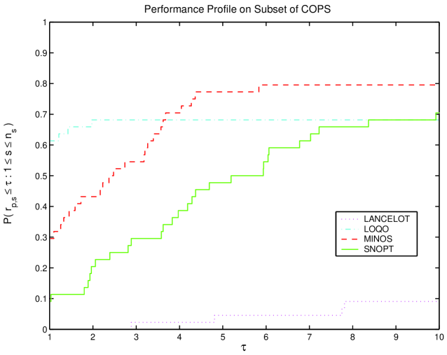
Figure 4.1: Performance profile on $[0,10]$

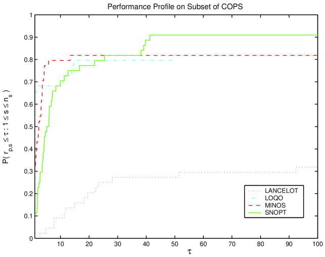
Figure 4.2: Performance profile on $[0,100]$

Figure 4.1 shows the performance profiles of the four solvers for small values of $\tau$. By showing the ratios of solver times, we eliminate any weight of importance that taking straight time differences might give to the problems that require a long run time of every solver. We find no need to eliminate any test problems from discussion. For this reason, solvers receive their due credit for completing problems for which one or more of the other solvers fails. In particular, $1-\rho_{s}(\tau)$ is the fraction of problems that the solver cannot solve within a factor $\tau$ of the best solver, including problems for which the solver in question fails.

From this figure it is clear that LOQO has the most wins (has the highest probability of being the optimal solver) and that the probability that LOQO is the winner on a given problem is about $.61$. If we choose being within a factor of $4$ of the best solver as the scope of our interest, then either LOQO or MINOS would suffice; but the performance profile shows that the probability that these two solvers can solve a job within a factor $4$ of the best solver is only about $70\%$. SNOPT has a lower number of wins than either LOQO or MINOS, but its performance becomes much more competitive if we extend our $\tau$ of interest to $7$.

Figure 4.2 shows the performance profiles for all the solvers in the interval $[1,100]$. If we are interested in the solver that can solve $75\%$ of the problems with the greatest efficiency, then MINOS stands out. If we hold to more stringent probabilities of completing a solve successfully, then SNOPT captures our attention with its ability to solve over $90\%$ of this COPS subset, as displayed by the height of its performance profile for $\tau>40$. This graph displays the potential for large discrepancies in the performance ratios on a substantial percentage of the problems. Another point of interest is that LOQO, MINOS, and SNOPT each have the best probability $\rho_{s}(\tau)$ for $\tau$ in some interval, with similar performance in the interval $[15,40]$.

An observation that emerges from these figures is the lack of consistency in quartile values of time ratios. The top three solvers share a minimum ratio of $1$, and LOQO and MINOS also share first quartile values of $1$. In other words, these two solvers are the best solvers on at least 25% of the problems. LOQO bests MINOS’s median value with $1$ compared with $2.4$, but MINOS comes back with a third quartile ratio of $4.3$ versus $13.9$ for LOQO, with SNOPT mixing results further by also beating LOQO with $12.6$. By looking at Figures 4.1 and 4.2, we see that progress between quartiles does not necessarily proceed linearly; hence, we really lose information if we do not provide the full data. Also, the maximum ratio would be $r_{M}$ for our testing, and no obvious alternative value exists. As an alternative to providing only quartile values, however, the performance profile yields much more information about a solver’s strengths and weaknesses.

We have seen that at least two graphs may be needed to examine the performance of the solvers. Even extending $\tau$ to $100$, we fail to capture the complete performance data for LANCELOT and LOQO. As a final option, we display a log scale of the performance profiles. In this way, we can show all activity that takes place with $\tau<r_{M}$ and grasp the full implications of our test data regarding the solvers’ probability of successfully handling a problem. Since we are also interested in the behavior for $\tau$ close to unity, we use a base of 2 for the scale. In other words, we plot

$$\tau\mapsto\frac{1}{n_{p}}\mbox{size}\left\{p\in\mbox{$\cal P$}:\log_{2}\left(r_{p,s}\right)\leq\tau\right\}$$

in Figure 4.3. This graph reveals all the features of the previous two graphs and thus captures the performance of all the solvers. The disadvantage is that the interpretation of the graph is not as intuitive, since we are using a log scale.

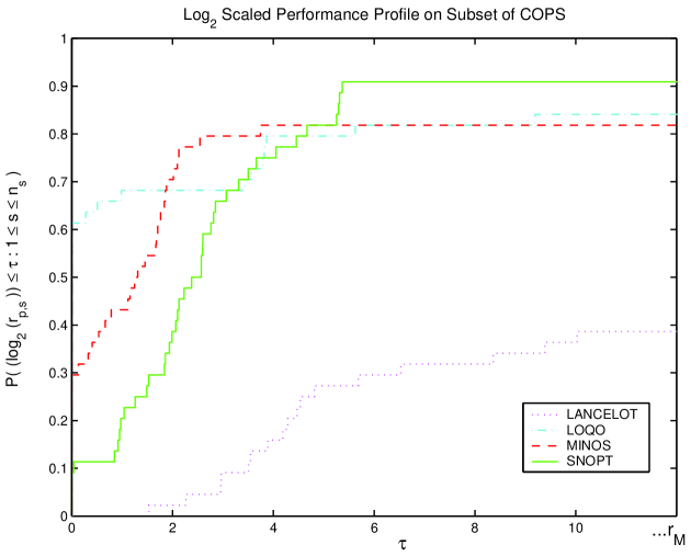
Figure 4.3: Performance profile in a $\log_{2}$ scale

Figures 4.1 and 4.2 are mapped into a new scale to reflect all data, requiring at least the interval $[0,\log_{2}(1043)]$ in Figure 4.3 to include the largest $r_{p,s}<r_{M}$. We extend the range slightly to show the flatlining of all solvers. The new figure contains all the information of the other two figures and, in addition, shows that each of the solvers fails on at least $8\%$ of the problems. This is not an unreasonable performance for the COPS test set because these problems were generally chosen to be difficult.

5 Case Study: The Full COPS

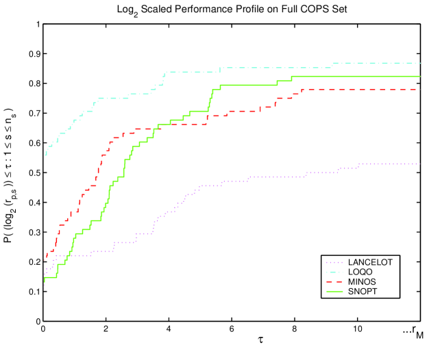
Figure 5.1: Performance profile for full COPS set

We now expand our analysis of the data to include all the problems in version 2.0 of the COPS cops-home test set. We present in Figure 5.1 a log₂ scaled view of the performance profiles for the solvers on that test set.

Figure 5.1 gives a clear indication of the relative performance of each solver. As in the performance profiles in Section 4, this figure shows that performance profiles eliminate the undue influence of a small number of problems on the benchmarking process and the sensitivity of the results associated with the ranking of solvers. In addition, performance profiles provide an estimate of the expected performance difference between solvers.

The most significant aspect of Figure 5.1, as compared with Figure 4.3, is that on this test set LOQO dominates all other solvers: the performance profile for LOQO lies above all others for all performance ratios. The interpretation of the results in Figure 5.1 is important. In particular, these results do not imply that LOQO is faster on every problem. They indicate only that, for any $\tau\geq 1$, LOQO solves more problems within a factor of $\tau$ of any other solver time. Moreover, by examining $\rho_{s}(1)$ and $\rho_{s}(r_{M})$, we can also say that LOQO is the fastest solver on approximately 58% of the problems, and that LOQO solves the most problems (about 87%) to optimality.

The difference between the results in Section 4 and these results is due to a number of factors. First of all, as can be seen in Table 3.1, the degrees of freedom for the full COPS test set is much larger than for the restricted subset of optimal control and parameter estimation problems. Since, as noted in Section 3, MINOS and SNOPT are designed for problems with a modest number of degrees of freedom, we should expect the performance of MINOS and SNOPT to deteriorate on the full COPS set. This deterioration can be seen by comparing Figure 5.1 with Figure 4.3 and noting that the performance profiles of MINOS and SNOPT are similar but generally lower in Figure 5.1.

Another reason for the difference between the results in Section 4 and these results is that MINOS and SNOPT use only first-order information, while LOQO uses second-order information. The benefit of using second-order information usually increases as the number of variables increases, so this is another factor that benefits LOQO.

The results in this section underscore our observation that performance profiles provide a convenient tool for comparing and evaluating the performance of optimization solvers, but, like all tools, performance profiles must be used with care. A performance profile reflects the performance only on the data being used, and thus it is important to understand the test set and the solvers used in the benchmark.

6 Case Study: Linear Programming

Performance profiles can be used to compare the performance of two solvers, but performance profiles are most useful in comparing several solvers. Because large amounts of data are generated in these situations, trends in performance are often difficult to see. As a case study, we use data obtained by Mittelmann Benchmarks. Figure 6.1 shows a plot of the performance profile for the time ratios in the data Benchmark of LP solvers on a Linux-PC (5-25-2000), which includes results for COPL_LP (1.0), PCx (1.1), SOPLEX (1.1), LPABO (5.6), MOSEK (1.0b), BPMPD (2.11), and BPMPD (2.14).

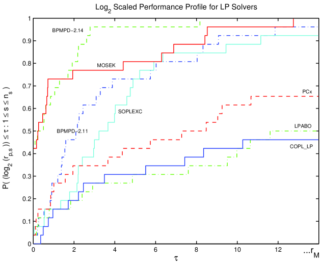
Figure 6.1: Performance profile for linear programming solvers

In keeping with our graphing practices with the COPS set, we designate as failures those solves that are marked in the original table as stopping close to the final solution without convergence under the solver’s stopping criteria. One feature we see in the graph of Mittelmann’s results that does not appear in the COPS graphs is the visual display of solvers that never flatline. In other words, the solvers that climb off the graph are those that solve all of the test problems successfully. As with Figure 4.3, all of the events in the data fit into this log-scaled representation. While this data set cannot be universally representative of benchmarking results by any means, it does show that our reporting technique is applicable beyond our own results.

As in the case studies in Sections 4 and 5, the results in Figure 6.1 give an indication of the performance of LP solvers only on the data set used to generate these results. In particular, the test set used to generate Figure 6.1 includes only problems selected by Mittelmann for his benchmark. The advantage of these results is that, unlike the solvers in Sections 4 and 5, all solvers in Figure 6.1 have the same requirements.

7 Conclusions

We have shown that performance profiles combine the best features of other tools for benchmarking and comparing optimization solvers. Clearly, the use of performance profiles is not restricted to optimization solvers and can be used to compare solvers in other areas.

We have not addressed the issue of how to select a collection of test problems to justify performance claims. Instead, we have provided a tool – performance profiles – for evaluating the performance of two or more solvers on a given set of test problems. If the data is obtained by following careful guidelines Crowder:1979:RCE; JacBNP91, then performance profiles can be used to justify performance claims. We emphasize that claims on the relative performance of the solvers on problems not in the test set should be made with care.

The Perl script perf.pl on the COPS site cops-home generates performance profiles formatted as Matlab commands to produce a composite graph as in Figures 4.1 and 4.2. The script accepts data for several solvers and plots the performance profile on an interval calculated to show the full area of activity. The area displayed and scale of the graph can then be adjusted within Matlab to reflect particular benchmarking interests.