Linear-Time Succinct Encodings of Planar Graphs
via Canonical Orderings

Abstract

Let $G$ be an embedded planar undirected graph that has $n$ vertices, $m$ edges, and $f$ faces but has no self-loop or multiple edge. If $G$ is triangulated, we can encode it using $\frac{4}{3}m-1$ bits, improving on the best previous bound of about $1.53m$ bits. In case exponential time is acceptable, roughly $1.08m$ bits have been known to suffice. If $G$ is triconnected, we use at most $(2.5+2\log{3})\min\{n,f\}-7$ bits, which is at most $2.835m$ bits and smaller than the best previous bound of $3m$ bits. Both of our schemes take $O(n)$ time for encoding and decoding.

1 Introduction

This paper investigates the problem of encoding a given graph $G$ into a binary string $S$ with the requirement that $S$ can be decoded to reconstruct $G$. The problem has been studied generally with two primary objectives. One is to minimize the length of $S$, while the other is to minimize the time needed to compute and decode $S$. In light of these goals, a coding scheme is efficient if its encoding and decoding procedures both take polynomial time. A coding scheme is succinct if the length of $S$ is not much larger than its information-theoretic tight bound, i.e., the shortest length over all possible coding schemes.

As the two primary objectives are often in conflict, a number of coding schemes with different trade-offs have been proposed from practical and theoretical perspectives. The most well-known efficient succinct scheme is the folklore scheme of encoding a rooted ordered $n$-vertex tree into a string of balanced $n-1$ pairs of left and right parentheses, which uses $2(n-1)$ bits. Since the total number of such trees is at least $\frac{1}{2(n-1)}{\cdot}\frac{(2n-2)!}{(n-1)!(n-1)!}$, the minimum number of bits needed to differentiate these trees is the logarithm of this quantity, which is $2n-o(n)$ by Stirling’s approximation. Thus, 2 bits per edge is an information-theoretic tight bound for encoding rooted ordered trees. The standard adjacency-list encoding of a graph is widely useful but requires $\Theta(m{\log}n)$ bits where $m$ and $n$ are the numbers of edges and vertices, respectively [3]. For certain graph families, Kannan, Naor and Rudich [10] gave schemes that encode each vertex with $O(\log n)$ bits and support $O(\log n)$-time testing of adjacency between two vertices. For connected planar graphs, Jacobson [9] gave an $\Theta(n)$-bit encoding which supports traversal in $\Theta(\log{n})$ time per vertex visited. This result was recently improved by Munro and Raman [17]; their schemes encode binary trees, rooted ordered trees and planar graphs succinctly and support several graph operations in constant time. For dense graphs and complement graphs, Kao, Occhiogrosso, and Teng [14] devised two compressed representations from adjacency lists to speed up basic graph techniques such as breadth-first search and depth-first search. Galperin and Wigderson [6] and Papadimitriou and Yannakakis [19] investigated complexity issues arising from encoding a graph by a small circuit that computes its adjacency matrix. For labeled planar graphs, Itai and Rodeh [8] gave an encoding procedure that requires $\frac{3}{2}n\log n+O(n)$ bits. For unlabeled general graphs, Naor [18] gave an encoding of $\frac{n^{2}}{2}-n\log{n}+O(n)$ bits, which is optimal to the second order.

Our work aims to minimize the number of bits needed to encode an embedded planar graph $G$ which is unlabeled and undirected. We assume that $G$ has $n$ vertices, $m$ edges, and $f$ faces but has no self-loop or multiple edge. (See [2, 7, 16] for the graph-theoretic terminology used in this paper.) Note that if polynomial time for encoding and decoding is not required, then any given graph in a large family can be encoded with the information-theoretic minimum number of bits by brute-force enumeration. This paper focuses on schemes that use only $O(n)$ time for both encoding and decoding.

For a general planar graph $G$, Turán [21] gave an encoding using $4m$ bits asymptotically. This space complexity was improved by Keeler and Westbrook [15] to about $3.58m$ bits. They also gave encoding algorithms for several important classes of planar graphs. In particular, they showed that if $G$ is triangulated, it can be encoded in about $1.53m$ bits. If $G$ is triconnected, it can be encoded using $3m$ bits. In this paper, these latter two results are improved as follows. If $G$ is triangulated, it can be encoded using $\frac{4}{3}m-1$ bits. It is interesting that rooted ordered trees require 2 bits per edge, while the seemingly more complex plane triangulations need fewer bits. Note that Tutte [22] gave an enumeration theorem that yields an information-theoretic tight bound of roughly $1.08m$ bits for plane triangulations that may contain multiple edges. If $G$ is triconnected, we can encode it using at most $(2.5+2\log{3})\min\{n,f\}-7$ bits, which is at most $2.835m$ bits. Both of our coding schemes are intuitive and simple. They require only $O(n)$ time for encoding as well as decoding. The schemes make new uses of the canonical orderings of planar graphs, which were originally introduced by de Fraysseix, Pach and Pollack [4] and extended by Kant [11]. These structures and closely related ones have proven useful also for drawing planar graphs in organized and compact manners [12, 13, 20].

This paper is organized as follows. In §2, we present our coding scheme for plane triangulations. In §3, we generalize the scheme to encode triconnected plane graphs. We conclude the paper with some open problems in §4.

2 A Coding Scheme for Plane Triangulations

This section assumes that $G$ is a plane triangulation. Thus, $n\geq 3$ and $G$ has $m=3n-6$ edges.

Let $v_{1},\ldots,v_{n}$ be an ordering of the vertices of $G$, where $v_{1},v_{2},v_{n}$ are the three exterior vertices of $G$ in the counterclockwise order. After fixing such an ordering, let $G_{k}$ be the subgraph of $G$ induced by $v_{1},\ldots,v_{k}$. Let $H_{k}$ be the exterior face of $G_{k}$. Let $G-G_{k}$ be the subgraph of $G$ obtained by removing $v_{1},\ldots,v_{k}$. Our coding scheme uses a special kind of ordering defined as follows.

Definition 1 (see [4]).

An ordering $v_{1},\ldots,v_{n}$ of $G$ is canonical if the following statements hold for every $k=3,\ldots,n$:

1. $G_{k}$ is biconnected, and its exterior face $H_{k}$ is a cycle containing the edge $(v_{1},v_{2})$.

2. The vertex $v_{k}$ is on the exterior face of $G_{k}$, and the set of its neighbors in $G_{k-1}$ forms a subinterval of the path $H_{k-1}-\{(v_{1},v_{2})\}$ and consists of at least two vertices. Furthermore, if $k<n$, $v_{k}$ has at least one neighbor in $G-G_{k}$. Note that the case $k=3$ is somewhat ambiguous due to degeneracy, and $H_{2}-\{(v_{1},v_{2})\}$ is regarded as the edge $(v_{1},v_{2})$ itself.

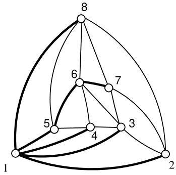
Fig. 1: A plane triangulation and a canonical ordering.

Figure 1 illustrates a canonical ordering of a plane triangulation. Note that every plane triangulation has a canonical ordering which can be computed in $O(n)$ time [4]. A canonical ordering of $G$ can be viewed as an order in which $G$ is reconstructed from a single edge $(v_{1},v_{2})$ step by step. At step $k$ with $3\leq k\leq n$, the vertex $v_{k}$ and the edges between $v_{k}$ and its lower ordered neighbors are added into the graph. For the sake of enhancing intuitions, we call $H_{k-1}$ the contour of $G_{k-1}$; denote its vertices by $c_{1}(=v_{1}),c_{2},\ldots,c_{t-1},c_{t}(=v_{2})$ in the consecutive order along the cycle $H_{k-1}$; and visualize them as arranged from left to right above the edge $(v_{1},v_{2})$ in the plane. When the vertex $v_{k}$ is added to $G_{k-1}$ to construct $G_{k}$, let $c_{\ell},c_{\ell+1},\ldots,c_{r}$ be the neighbors of $v_{k}$ on the contour $H_{k-1}$. After $v_{k}$ is added, the vertices $c_{\ell+1},\ldots,c_{r-1}$ are no longer contour vertices. Thus, we say that these vertices are covered by $v_{k}$. The edge $(v_{k},c_{\ell})$ is the left edge of $v_{k}$; the edge $(v_{k},c_{r})$ is the right edge of $v_{k}$; the edges $(c_{p},v_{k})$ with $\ell<p<r$ are the internal edges of $v_{k}$.

There is no published reference for the following folklore lemma; for the sake of completeness, we include its proof here.

Lemma 2.

Let $v_{1},\ldots,v_{n}$ be a canonical ordering of $G$. Let $T_{1}$ $($respectively, $T_{2}$$)$ be the collection of the left $($respectively, right$)$ edges of $v_{j}$ for $3\leq j\leq n-1$; similarly, let $T_{n}$ be that of the internal edges of $v_{j}$ for $3\leq j\leq n$.

1. $T_{1}$ is a tree spanning over $G-\{v_{2},v_{n}\}$.

2. $T_{2}$ is a tree spanning over $G-\{v_{1},v_{n}\}$.

3. $T_{n}$ is a tree spanning over $G-\{v_{1},v_{2}\}$.

Proof.

The statements are proved separately as follows.

Statement 1. For $i=3,\ldots,n-1$, let $D_{i}$ be the collection of the left edges of $v_{j}$ for $3\leq j\leq i$. We prove by induction on $i$ the claim that $D_{i}$ is a tree spanning over $v_{1},v_{3},\ldots,v_{i}$. Then, since $T_{1}=D_{n-1}$, the claim implies the statement. For the base case $i=3$, the claim trivially holds. The induction hypothesis is that the claim holds for $i=k-1<n-1$. The induction step is to prove the claim for $i=k\leq n-1$. $D_{k}$ is obtained from $D_{k-1}$ by adding the left edge $(v_{k},c_{\ell})$ of $v_{k}$. By the induction hypothesis, $D_{k-1}$ is a tree spanning over $v_{1},v_{3},\ldots,v_{k-1}$. Since $c_{\ell}$ is the leftmost neighbor of $v_{k}$ on $H_{k-1}$, $c_{\ell}$ is some $v_{j}$ with $1\leq j\leq k-1$ and $j\not=2$. Thus, $D_{k-1}$ contains $c_{\ell}$, and $D_{k}$ is a tree spanning over $v_{1},v_{3},\ldots,v_{k-1},v_{k}$.

Statement 2. The proof is symmetric to that of Statement 1.

Statement 3. $G$ has $n$ vertices and $3n-6$ edges. The edges $(v_{1},v_{2}),(v_{2},v_{n}),(v_{1},v_{n})$ are not in $T_{1}\cup T_{2}\cup T_{n}$. Thus, since $T_{1}$ and $T_{2}$ have $n-3$ edges each, $T_{n}$ has $n-3$ edges. Then, since $T_{n}$ is acyclic and does not contain $v_{1}$ and $v_{2}$, $T_{n}$ is a spanning tree of $G-\{v_{1},v_{2}\}$. ∎

A canonical ordering $v_{1},\ldots,v_{n}$ is rightmost if for all $v_{k}$ and $v_{k^{\prime}}$ with $k^{\prime}>k$ such that the neighbors of $v_{k^{\prime}}$ on $H_{k^{\prime}-1}$ are all in $H_{k-1}$, the leftmost neighbor of $v_{k^{\prime}}$ appears before that of $v_{k}$ when traversing $H_{k-1}$ from $v_{1}$ to $v_{2}$ in the clockwise direction. Intuitively speaking, if there are more than one vertex that can be added to $G_{k-1}$, we always add the rightmost one. The ordering in Figure 1 is rightmost. A rightmost canonical ordering is symmetric to a leftmost one in [11] and can be computed from $G$ in linear time similarly.

Let $v_{1},\ldots,v_{n}$ be a rightmost canonical ordering of $G$. Let $T_{1}$ be as in Lemma 2 for this ordering. Let $T$ be the tree $T_{1}\cup\{(v_{1},v_{n}),(v_{1},v_{2})\}$. In Figure 1, $T$ is indicated by the thick lines. Our coding scheme uses $T$ extensively. The rightmost depth-first search of $T$ proceeds as follows. We start at $v_{1}$ and traverse the edge $(v_{1},v_{2})$ first. Afterwards, if two or more vertices can be visited from $v_{k}$, we choose the rightmost one. More precisely, let $P$ be the path in $T$ from $v_{k}$ to $v_{1}$ and then to $v_{2}$. Let $D$ be the set of edges between $v_{k}$ and the available vertices. We visit a new vertex through the edge in $D$ that is next to $P$ in the counterclockwise cyclic order around $v_{k}$ formed by $P$ and the edges in $D$. Note that the order in which the vertices are visited by the rightmost depth-first search is the rightmost canonical ordering $v_{1},\ldots,v_{n}$ that defines $T$.

We are now ready to describe the encoding $S$ of $G$ as the concatenation of two binary strings $S_{1}$ and $S_{2}$ as follows.

$S_{1}$ is the binary string that encodes $T$ using the folklore parenthesis coding scheme where $0$ and $1$ correspond to ${}^{\prime\prime}(^{\prime\prime}$ and ${}^{\prime\prime})^{\prime\prime}$, respectively. In this encoding, $T$ is rooted at $v_{1}$, and the branches are ordered the same as their enpoints are in the rightmost canonical ordering. Since $T$ contains $n$ vertices, $S_{1}$ has $2(n-1)$ bits.

$S_{2}$ encodes the number of contour vertices covered by each $v_{k}$ with $3\leq k\leq n$. First, we create a string of $n-2$ copies of $0$. The $(k-2)$-th $0$ corresponds to $v_{k}$. If $v_{k}$ covers $d$ vertices, we insert $d$ copies of $1$ before the corresponding $0$. For example, the string $S_{2}$ for Figure 1 is:

$$00010101110$$

Since each vertex $v_{k}$ with $3\leq k\leq n-1$ is covered exactly once, $S_{2}$ has $n-3$ copies of 1. So $|S_{2}|=(n-2)+(n-3)=2n-5$ bits. Hence, $|S|=|S_{1}|+|S_{2}|=4n-7$ bits.

We next describe how to decode $S$ to reconstruct $G$. Given $S$, we can uniquely determine $n$ from the length of $S$. Subsequently, we can uniquely determine $S_{1}$ and $S_{2}$. From $S_{1}$, we can reconstruct $T$. From $T$, we can recover the ordering $v_{1},\ldots,v_{n}$. Then, we draw the edge $(v_{1},v_{2})$ and perform a loop of $n-2$ steps indexed by $k$ with $3\leq k\leq n$ where step $k$ processes $v_{k}$. Before $v_{k}$ is processed, $G_{k-1}$ and its contour $H_{k-1}$ have been constructed. At step $k$, we add $v_{k}$ and the edges between $v_{k}$ and its lower ordered neighbors into $G_{k-1}$ to construct $G_{k}$ as follows. From $T$, we can identify the leftmost neighbor $c_{\ell}$ of $v_{k}$ on the contour $H_{k-1}$, because $c_{\ell}$ is simply the parent of $v_{k}$ in $T$. From $S_{2}$, we can determine the number $d$ of vertices covered by $v_{k}$. Thus, we add the edges $(c_{\ell},v_{k}),(c_{\ell+1},v_{k}),\ldots,(c_{\ell+d+1},v_{k})$ into $G_{k-1}$; note that $r=\ell+d+1$. This gives us the subgraph $G_{k}$ and completes step $k$.

It is straightforward to carry out these encoding and decoding procedures in linear time. Also, we can save 1 bit by deleting the last $0$ in $S_{2}$. Since $v_{3}$ covers no vertex, for $n\geq 4$, we can save another bit by deleting the first $0$ in $S_{2}$. Note that for $n=3$, the last $0$ in $S_{2}$ is also the first $0$ and cannot be deleted twice, but we can simply encode the 3-vertex plane triangulation with zero bit without ambiguity. Thus, we have the following theorem.

Theorem 3.

A plane triangulation of $m$ edges and $n$ vertices with $n\geq 4$ can be encoded using $4n-9=\frac{4}{3}m-1$ bits. Both encoding and decoding take $O(n)$ time.

3 A Coding Scheme for Triconnected Plane Graphs

This section assumes that $G$ is triconnected. To avoid triviality, let $n\geq 3$.

Let $v_{1},\ldots,v_{n}$ be an ordering of the vertices of $G$ where $v_{1},v_{2},v_{n}$ are on the exterior face of $G$, and $v_{2}$ and $v_{n}$ are neighbors of $v_{1}$. Let $G_{k}$ be the subgraph of $G$ induced by $v_{1},\ldots,v_{k}$. Let $H_{k}$ be the exterior face of $G_{k}$. Let $G-G_{k}$ be the subgraph of $G$ obtained by removing $v_{1},\ldots,v_{k}$. Our coding scheme for triconnected plane graphs uses an ordering defined as follows.

Definition 4 (see [11]).

An ordering $v_{1},\ldots,v_{n}$ of a triconnected plane graph $G$ is canonical if the integer interval $[3,n]$ can be partitioned into subintervals $[k,k+q]$ each satisfying either set of properties below:

1. The integer $q$ is $0$. The vertex $v_{k}$ is on the exterior face of $G_{k}$ and has at least two neighbors in $G_{k-1}$. $G_{k}$ is biconnected and its exterior face contains the edge $(v_{1},v_{2})$. If $k<n$, $v_{k}$ has at least one neighbor in $G-G_{k}$.

2. The integer $q$ is at least $1$. The sequence $v_{k},v_{k+1},\ldots,v_{k+q}$ is a chain on the exterior face of $G_{k+q}$ and has exactly two neighbors in $G_{k-1}$, one for $v_{k}$ and the other for $v_{k+q}$, which are on the exterior face of $G_{k-1}$. $G_{k+q}$ is biconnected and its exterior face contains the edge $(v_{1},v_{2})$. Every vertex among $v_{k},\ldots,v_{k+q}$ has at least one neighbor in $G-G_{k+q}$.

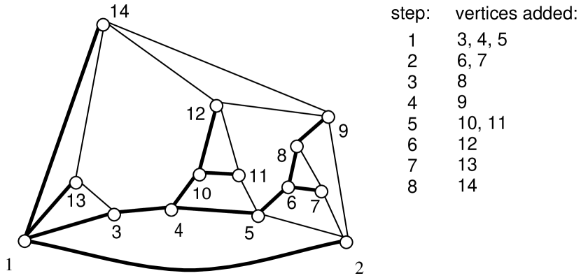
Fig. 2: A triconnected plane graph and a canonical ordering.

As in §2, we similarly define a rightmost canonical ordering $v_{1},\ldots,v_{n}$ of $G$. Figure 2 shows a rightmost canonical ordering of a triconnected plane graph. Given a triconnected plane graph, we can find a rightmost canonical ordering in linear time [11]. With a rightmost canonical ordering, $G$ can be reconstructed from a single edge $(v_{1},v_{2})$ through a sequence of steps indexed by $k^{\prime}$. There are two possible cases at step $k^{\prime}$, which correspond to the two sets of properties in Definition 4 and are used throughout this section.

Case 1: A single vertex $v_{k}$ is added.

Case 2: A chain of $q+1$ vertices $v_{k},\ldots,v_{k+q}$ is added.

While reconstructing $G$, we collect a set $T$ of edges as follows. Initially, $T$ consists of the edge $(v_{1},v_{2})$. Let $c_{1}(=v_{1}),c_{2},\ldots,c_{t-1},c_{t}(=v_{2})$ be the vertices of $H_{k-1}$, which are ordered consecutively along the boundary cycle of $H_{k-1}$ and are arranged from left to right above the edge $(v_{1},v_{2})$ in the plane.

Case 1. Let $c_{\ell}$ and $c_{r}$ with $1\leq\ell<r\leq t$ be the leftmost and rightmost neighbors of $v_{k}$ in $H_{k-1}$, respectively. After $v_{k}$ is added, $c_{\ell+1},\ldots,c_{r-1}$ are no longer contour vertices; these vertices are covered at step $k^{\prime}$. The edge $(c_{\ell},v_{k})$ is included in $T$.

Case 2. Let $c_{\ell}$ and $c_{r}$ with $1\leq\ell<r\leq t$ be the neighbors of $v_{k}$ and $v_{k+q}$ in $H_{k-1}$, respectively. After $v_{k},\ldots,v_{k+q}$ are added, $c_{\ell+1},\ldots,c_{r-1}$ are no longer contour vertices; these vertices are covered at step $k^{\prime}$. The edges $(c_{\ell},v_{k}),(v_{k},v_{k+1}),\ldots,(v_{k+q-1},$ $v_{k+q})$ are included in $T$.

In Figure 2, the edges in $T$ are indicated by the thick lines. By an argument similar to the proof of Lemma 2(1), $T$ is a spanning tree of $G$. As in §2, we similarly define the rightmost depth-first search in $T$. Note that the order in which the vertices of $T$ are visited by the rightmost depth-first search is the rightmost canonical ordering $v_{1},\ldots,v_{n}$ that defines $T$.

We are now ready to describe the encoding $S$ of $G$ by means of $T$. We further divide Case 1 into three subcases.

Case 1a: No vertex is covered at step $k^{\prime}$.

Case 1b: At least one vertex is covered at step $k^{\prime}$ and the leftmost covered vertex $c_{\ell+1}$ is adjacent to $v_{k}$.

Case 1c: At least one vertex is covered at step $k^{\prime}$ and the leftmost covered vertex $c_{\ell+1}$ is not adjacent to $v_{k}$.

Let $\beta$ be the number of steps for reconstructing $G$. Let $\beta_{1a},\beta_{1b},\beta_{1c}$ and $\beta_{2}$ be the numbers of steps of Cases 1a, 1b, 1c, and 2, respectively. We first consider the case $\beta_{1b}\geq\beta_{1c}$ to encode $G$ with Scheme I; afterwards, we modify Scheme I into Scheme II for the case $\beta_{1b}<\beta_{1c}$.

In Scheme I, the encoding $S$ of $G$ is the concatenation of three strings $S_{1}$, $S_{2}$ and $S_{3}$. $S_{1}$ is the folklore parentheses encoding of $T$, which is rooted and ordered in the same way as in §2. Since $T$ has $n$ vertices, $S_{1}$ has $2(n-1)$ bits.

To construct $S_{2}$, first let $Q=s_{1}*s_{2}*\cdots*s_{\beta}*$ where each $s_{k^{\prime}}$ is a binary string that corresponds to the step $k^{\prime}$ of reconstructing $G$ based on the ordering $v_{1},\ldots,v_{n}$. $s_{k^{\prime}}$ is determined as follows. The following two cases both assume that $d$ vertices are covered at step $k^{\prime}$.

Case 1. Note that $d=r-\ell-1$. The string $s_{k^{\prime}}$ has $d$ symbols corresponding to $c_{j}$ with $j=\ell+1,\ldots,r-1$, respectively. If the edge $(c_{j},v_{k})$ is present in $G$, the symbol in $s_{k^{\prime}}$ corresponding to $c_{j}$ is 1; otherwise, the symbol is 0. Note that in Case 1a, since no vertex is covered, $s_{k^{\prime}}$ is empty.

Case 2. The string $s_{k^{\prime}}$ consists of $q$ copies of $0$ followed by $d$ copies of $1$.

For example, the string $Q$ for Figure 2 is:

$\begin{array}[]{cccccccccccccc}\underbrace{00}&*&0&*&*&0&*&0&*&\underbrace{1000}&*&*&\underbrace{10001}&*\\ \uparrow&&\uparrow&&&\uparrow&&\uparrow&&\uparrow&&&\uparrow&\\ s_{1}&&s_{2}&&&s_{4}&&s_{5}&&s_{6}&&&s_{8}&\\ \end{array}$

$S_{2}$ is a binary representation of $Q$ defined as follows. A step of Case 1 adds one vertex to $G$ and correspondingly includes one $*$ in $Q$; similarly, a step of Case 2 adds $q+1$ vertices to $G$ and includes one $*$ and $q$ copies of $0$ in $Q$. Since exactly $n-2$ vertices are added, the total number of these symbols is $n-2$. Each symbol in $Q$ not yet counted corresponds to a vertex covered at the $\beta$ steps. Since each $v_{k}$ with $3\leq k\leq n-1$ is covered at most once and $v_{1},v_{2},v_{n}$ are never covered, the total number of these latter symbols is at most $n-3$. Thus $Q$ has at most $2n-5$ symbols. For the sake of unambiguous decoding, we pad $Q$ with copies of 1 at its end to have exactly $2n-5$ symbols. Since $Q$ uses 3 distinct symbols, we treat it as an integer of base 3 and convert it to a binary integer. Again, for the sake of unambiguous decoding, we use exactly $\lceil{(2n-5)\log{3}}\rceil$ bits for this binary integer by padding copies of $0$ at its beginning. The resulting binary string is the desired $S_{2}$.

For the sake of decoding, we also need to know whether any given $s_{k^{\prime}}$ is of Case 1 or 2. Thus, let $S_{3}=t_{1}\cdots t_{\beta}$ where $t_{k^{\prime}}=1$ if step $k^{\prime}$ is of Case 1 and $t_{k^{\prime}}=0$ otherwise. To save space, note that some bits $t_{k^{\prime}}$ can be deleted as follows without incurring ambiguity. If step $k^{\prime}$ is of Case 1a, $t_{k^{\prime}}$ is deleted because $s_{k^{\prime}}$ is empty and only a string of Case 1a can be empty. If step $k^{\prime}$ is of Case 1b, $t_{k^{\prime}}$ is deleted because $s_{k^{\prime}}$ starts with 1, while the strings of Case 2 start with 0. If step $k^{\prime}$ is of Case 1c or 2, $t_{k^{\prime}}$ remains in $S_{3}$. For example, the string $S_{3}$ for Figure 2 consists of $t_{1}=0$, $t_{2}=0$, $t_{4}=1$, $t_{5}=0$. Thus, $S_{3}$ has $\beta_{1c}+\beta_{2}$ bits, which can be bounded as follows. A step of Case 1 adds one vertex into $G$ and a step of Case 2 adds at least two vertices. Since $n-2$ vertices are added over the $\beta$ steps, $\beta_{1a}+\beta_{1b}+\beta_{1c}+2\beta_{2}\leq n-2$. Since Scheme I assumes $\beta_{1b}\geq\beta_{1c}$, $|S_{3}|=\beta_{1c}+\beta_{2}\leq\frac{1}{2}{\cdot}(\beta_{1b}+\beta_{1c})+\beta_{2}\leq\frac{1}{2}{\cdot}(\beta_{1a}+\beta_{1b}+\beta_{1c}+2\beta_{2})\leq 0.5n-1$.

Since $S=S_{1}//S_{2}//S_{3}$, $|S|\leq 2(n-1)+\lceil(2n-5)\log 3\rceil+0.5n-1\leq(2.5+2\log 3)n-9$ bits. This completes the description of the encoding procedure of Scheme I.

Next we describe how to decode $S$ to reconstruct $G$. This decoding assumes that both $S$ and $n$ are given. Thus, we can uniquely determine $S_{1}$, $S_{2}$ and $S_{3}$. Then we convert $S_{2}$ to $Q$. From $Q$ we can recover all $s_{k^{\prime}}$ with $1\leq k^{\prime}\leq\beta$. From $S_{3}$ and all $s_{k^{\prime}}$, we can recover all $t_{k^{\prime}}$ with $1\leq k^{\prime}\leq\beta$. From $S_{1}$, we reconstruct $T$. From $T$, we find the ordering $v_{1},\ldots,v_{n}$. Afterwards, we draw the edge $(v_{1},v_{2})$ and perform a loop of steps as follows. Each step is indexed by $k^{\prime}$ and corresponds to step $k^{\prime}$ of reconstructing $G$ using the rightmost canonical ordering.

If $t_{k^{\prime}}=1$, step $k^{\prime}$ is of Case 1. Thus, a vertex $v_{k}$ is added at this step where $v_{k}$ is the smallest ordered vertex not added into the current graph yet. From $T$, we can determine the leftmost neighbor $c_{\ell}$ of $v_{k}$ in the contour $H_{k-1}$ because $c_{\ell}$ is the parent of $v_{k}$ in $T$. From $s_{k^{\prime}}$, we know the number of vertices covered by $v_{k}$ and hence the rightmost neighbor $c_{r}$ of $v_{k}$ in the contour $H_{k-1}$. From $s_{k^{\prime}}$, we also know which of the covered vertices are connected to $v_{k}$. These corresponding edges are added to $G$.

If $t_{k^{\prime}}=0$, step $k^{\prime}$ is of Case 2. Thus, a chain $v_{k},\ldots,v_{k+q}$ is added at this step where $v_{k}$ is the smallest ordered vertex not added into the current graph yet. The integer $q$ can be determined from the string $s_{k^{\prime}}$ by counting its leading copies of $0$. From $s_{k^{\prime}}$, we also know the number of vertices covered at step $k^{\prime}$, which is the count of $1$ in $s_{k^{\prime}}$. Thus, we know the neighbor $c_{r}$ of $v_{k+q}$ in the contour $H_{k-1}$. The chain is added accordingly.

This completes the decoding procedure of Scheme I. It is straightforward to implement the whole Scheme I in $O(n)$ time. If $\beta_{1b}<\beta_{1c}$, we use Scheme II to encode $G$, which is identical to Scheme I with the following differences. If step $k^{\prime}$ is of Case 2, $s_{k^{\prime}}$ consists of $q$ copies of 1 followed by $d$ copies of 0. Also, all bits $t_{k^{\prime}}$ for steps of Cases 1a and 1c are omitted from $S_{3}$ without incurring ambiguity since their corresponding strings $s_{k^{\prime}}$ either are empty or start with 0 while the strings of Cases 1b and 2 start with 1. We use one extra bit to encode whether we use Scheme I or II. Thus we have the following lemma.

Lemma 5.

Any triconnected plane graph with $n$ vertices can be encoded using at most $(2.5+2\log 3)n-8$ bits. Both encoding and decoding take $O(n)$ time. The decoding procedure assumes that both $S$ and $n$ are given.

We can improve Lemma 5 as follows. Let $G^{*}$ be the dual of $G$. $G^{*}$ has $f$ vertices, $m$ edges and $n$ faces. Since $G$ is triconnected, $G^{*}$ is also triconnected. Furthermore, if $n>3$, then $f>3$ and $G^{*}$ has no self-loop or multiple edge. Thus, we can use the coding scheme of Lemma 5 to encode $G^{*}$ with at most $(2.5+2\log 3)f-8$ bits. Since $G$ can be uniquely determined from $G^{*}$, to encode $G$, it suffices to encode $G^{*}$. To make $S$ shorter, for the case $n>3$, if $n\leq f$, we encode $G$ using at most $(2.5+2\log 3)n-8$ bits; otherwise, we encode $G^{*}$ using at most $(2.5+2\log 3)f-8$ bits. This new encoding has at most $(2.5+2\log{3})\min\{n,f\}-8$ bits. Since $\min\{n,f\}\leq\frac{n+f}{2}$, the bit count is at most $(1.25+\log 3)m-2$ by Euler’s formula $n+f=m+2$. For the sake of decoding, we use one extra bit to denote whether we encode $G$ or its dual. Note that if $n=3$, we can simply encode $G$ using zero bit without ambiguity. Thus we have proved the following theorem.

Theorem 6.

Any triconnected plane graph with $n$ vertices, $m$ edges and $f$ faces can be encoded using at most $(2.5+2\log{3})\min\{n,f\}-7\leq(1.25+\log{3})m-1$ bits. Both encoding and decoding take $O(n)$ time. The decoding procedure assumes that $S$ is given together with $n$ or $f$ as appropriate.

Remark. There are several ways to improve this coding scheme so that the decoding does not require $n$ as input. One is to use well-known data compression techniques to encode $n$ and append it to the beginning of $S$ using $\log n+O(\log\log n)$ bits [1, 5]. Another is to pad $S$ with copies of $1$ at its end so that it has exactly $\lceil(2.5+2\log{3})\min\{n,f\}\rceil-7$ bits. Then, since $2.5+2\log{3}>1$, given $S$ alone, we can uniquely determine $n$ or $f$ and proceed with the original decoding procedure. With the strings $s_{k^{\prime}}$, we can unambiguously identify the padded bits.

4 Open Problems

This paper leaves several problems open. Since plane triangulations are useful in many application areas, it would be particularly helpful to encode them in $O(n)$ time using close to $1.08m$ bits. Similarly, it would be significant to obtain a linear-time coding scheme for triconnected plane graphs using close to $2m$ bits. Note that Tutte [23] proved an information-theoretic tight bound of $2m+o(m)$ bits for triconnected plane graphs that may contain multiple edges and self-loops. More generally, it would be of interest to encode graphs in a given family in polynomial time using their information-theoretic minimum number of bits. Solving these problems will most likely lead to the discovery of new structural properties of graphs.

Acknowledgments. The authors are grateful to anonymous referees for helpful comments.

References

- [1] T. C. Bell, J. G. Cleary, and I. H. Witten, Text Compression, Prentice-Hall, Englewood Cliffs, NJ, 1990.
- [2] C. Berge, Graphs, North-Holland, New York, NY, second revised ed., 1985.
- [3] T. H. Cormen, C. L. Leiserson, and R. L. Rivest, Introduction to Algorithms, MIT Press, Cambridge, MA, 1990.
- [4] H. de Fraysseix, J. Pach, and R. Pollack, How to draw a planar graph on a grid, Combinatorica, 10 (1990), pp. 41–51.
- [5] P. Elias, Universal codeword sets and representations of the integers, IEEE Transactions on Information Theory, IT-21 (1975), pp. 194–203.
- [6] H. Galperin and A. Wigderson, Succinct representations of graphs, Information and Control, 56 (1983), pp. 183–198.
- [7] F. Harary, Graph Theory, Addison-Wesley, Reading, MA, 1972.
- [8] A. Itai and M. Rodeh, Representation of graphs, Acta Informatica, 17 (1982), pp. 215–219.
- [9] G. Jacobson, Space-efficient static trees and graphs, in Proceedings of the IEEE Thirtieth Annual Symposium on Foundations of Computer Science, 1989, pp. 549–554.
- [10] S. Kannan, M. Naor, and S. Rudich, Implicit representation of graphs, SIAM Journal on Discrete Mathematics, 5 (1992), pp. 596–603.
- [11] G. Kant, Drawing planar graphs using the -ordering, in Proceedings of the 33rd Annual IEEE Symposium on Foundations of Computer Science, 1992, pp. 101–110.
- [12] G. Kant and X. He, Regular edge labeling of 4-connected plane graphs and its applications in graph drawing problems, Theoretical Computer Science, 172 (1997), pp. 175–193.
- [13] M. Y. Kao, M. Fürer, X. He, and B. Raghavachari, Optimal parallel algorithms for straight-line grid embeddings of planar graphs, SIAM Journal on Discrete Mathematics, 7 (1994), pp. 632–646.
- [14] M. Y. Kao, N. Occhiogrosso, and S. H. Teng, Simple and efficient compression schemes for dense and complement graphs, Journal of Combinatorial Optimization, (1999). To appear.
- [15] K. Keeler and J. Westbrook, Short encodings of planar graphs and maps, Discrete Applied Mathematics, 58 (1995), pp. 239–252.
- [16] L. Lovász, An Algorithmic Theory of Numbers, Graphs and Convexity, Society for Industrial and Applied Mathematics, Philadelphia, PA, 1986.
- [17] J. I. Munro and V. Raman, Succinct representation of balanced parentheses, static trees and planar graphs, in Proceedings of the 38th Annual IEEE Symposium on the Foundations of Computer Science, 1997, pp. 118–126.
- [18] M. Naor, Succinct representations of general unlabeled graphs, Discrete Applied Mathematics, 28 (1990), pp. 303–307.
- [19] C. H. Papadimitriou and M. Yannakakis, A note on succinct representations of graphs, Information and Control, 71 (1986), pp. 181–185.
- [20] W. Schnyder, Embedding planar graphs on the grid, in Proceedings of the 1st Annual ACM-SIAM Symposium on Discrete Algorithms, 1990, pp. 138–148.
- [21] G. Turán, On the succinct representation of graphs, Discrete Applied Mathematics, 8 (1984), pp. 289–294.
- [22] W. T. Tutte, A census of planar triangulations, Canadian Journal of Mathematics, 14 (1962), pp. 21–38.
- [23] , A census of planar maps, Canadian Journal of Mathematics, 15 (1963), pp. 249–271.