Abstract

The three Power-Laws proposed by Faloutsos et al. (1999) are important discoveries among many recent works on finding hidden rules in the seemingly chaotic Internet topology. In this note, we want to point out that the first two laws discovered by Faloutsos et al. (1999, hereafter, Faloutsos’ Power Laws) are in fact equivalent. That is, as long as any one of them is true, the other can be derived from it, and vice versa. Although these two laws are equivalent, they provide different ways to measure the exponents of their corresponding power law relations. We also show that these two measures will give equivalent results, but with different error bars. We argue that for nodes of not very large out-degree($\leq 32$ in our simulation), the first Faloutsos’ Power Law is superior to the second one in giving a better estimate of the exponent, while for nodes of very large out-degree($>32$) the power law relation may not be present, at least for the relation between the frequency of out-degree and node out-degree.

1 Introduction

The past five years has been the golden time for the 30 year old Internet, during which it experienced fascinating evolution, both exponential growth in its traffic and endless expansion in its topology. Such growth makes more thorough and rigorous analysis of the nature of Internet traffic and topology an urgent task. It is also a very difficult one. It was ever believed that the mathematical theories for circuit switching telephone networks might be good enough for analyzing the Internet traffic and topology. However, later it was found that the Internet, as a package switching network, has very different nature and successful mathematical theories for the Internet can be quite different from those for telephone networks(see Willinger and Paxson(1998) for more details).

As the Internet grows at an astonishing speed, more and more high quality data have been collected in recent years. These data make thorough studies possible. The pioneering work by Leland et al. (1994) shows that the traffic of Local Area Network(LAN) appears to be self-similar at different scales. Discoveries of other self-similarities such as the one found in Wide Area Network(WAN) by Paxson and Floyd(1995) make Internet engineers and interested mathematicians contemplate that some special power laws such as the heavy tail distribution might be the hidden rules in Internet traffic(see Willinger and Paxson(1998) or Willinger, Paxson and Taqqu(1998)).

The discovery of three Power Laws by Faloutsos, Faloutsos and Faloutsos(1999) is one of the most recent work on the Internet topology. They view the Internet as an undirected graph. For each node in the graph, it has properties such as the out-degree. Faloutsos’ discovery is not just power laws for the large scale properties of the Internet, but rather the relationships between nodes at different scales, running from a host on a LAN to the range encompassed by the whole Internet. Without a doubt, such discovery is important not only to our understanding of the very nature of the rapidly growing Internet, but also to any reasonable simulations of LANs or WANs or the whole Internet.

Yet, as we will point out in section 2 of this note, the first two Power Laws in Faloutsos’ discovery are not independent to each other. In fact, they are equivalent so each one can be derived from the other. In section 3, we will go further to show that the data analysis in Faloutsos’ work toward discovering Power Law 1 is superior to the data analysis work done for Power Law 2, simply because the former data analysis will give more accurate estimate comparing to the later one. Conclusions are summarized in the last section, section 4.

2 Equivalence Between the first and the second Faloutsos’ Power Laws

Throughout this note, we adopt the notations used in Faloutsos’ work. The Internet is viewed as an undirected graph $G$, and the number of nodes and the number of edges in $G$ are $N$ and $E$, respectively. The out-degree of a node $v$, which is the number of edges incident to the node, is denoted by $d_{v}$. Note that in $G$, different nodes may have the same out-degree. That is, if we can group all the nodes which have the same out-degree $d$ and index the group, then for the nodes in the $l^{th}$ group, they have the same out-degree denoted by $dl$. The number of nodes in this $l^{th}$ group, which gives the frequency of appearances of out-degree $dl$ in $G$, is denoted by $f_{dl}$. Sometimes we just write $f_{d}$ to denote the frequency of $d$ in $G$. This is because the out-degree $d$, which always starts from 1 throughout this note, can be used to index the groups of nodes of different out-degrees, thus $f_{d}$ is the number of nodes in the $d^{th}$ group for out-degree $d$. The rank, $r_{v}$, of a node $v$ which has an out-degree $d$ is the global index of the node among all of the nodes in the order of decreasing out-degree.

The first and second Faloutsos’ Power Laws can be stated as

$$d_{v}=C_{1}r_{v}^{R}$$ (1)

and

$$f_{d}=C_{2}d^{O}$$ (2)

respectively. Here $C_{1}$ is a constant and can be determined by any given pair of $d_{v}$ and $r_{v}$ measured from data collected from the Internet. $C_{2}$ is another constant and can be calculated from a pair of $f_{d}$ and $d$. $R$ and $O$ are the two exponents of the Power Laws.

By definition, the frequency of out-degree $d$ in $G$, $f_{d}$, is related to the ranks of those nodes which have out-degree $d$. Suppose node $v_{d-1}$ is a node of out-degree $d-1$, and it is the last indexed node with rank $r_{v}^{\prime}$ in the group consisting of nodes which all have out-degree $d-1$. Further suppose that node $v_{d}$ is a node of out-degree $d$, and it is the last indexed node, with rank $r_{v}$, in the group consisting of nodes of out-degree $d$. Then $f_{d}$ is related to $r_{v}^{\prime}$ and $r_{v}$ through the relation

$$f_{d}=r_{v}^{\prime}-r_{v}.$$ (3)

We may re-write relation (1) as

$$r_{v}=\left(\frac{1}{C_{1}}\right)^{\frac{1}{R}}d_{v}^{\frac{1}{R}}.$$ (4)

Note that the first order approximation to the right hand side of (3) is in fact the first order derivative of the right hand side of (4) with respect to $d$:

$$f_{d}={r_{v}^{\prime}-r_{v}}\approx-\frac{1}{R}\left(\frac{1}{C_{1}}\right)^{\frac{1}{R}}d^{\frac{1}{R}-1}$$ (5)

From (4) to (5) we changed $d_{v}$ to $d$ because for all nodes of the group where node $v_{d}$ is in, they all have the same out-degree $d$. Comparing (5) and (2), we have

$$O\approx\frac{1}{R}-1$$ (6)

and

$$C_{2}\approx-\frac{1}{R}\left(\frac{1}{C_{1}}\right)^{\frac{1}{R}}.$$ (7)

Thus we have derived the second Power Law from the first Power Law. To derive the first Power Law from the second, we have to integrate relation (2) from 1 to $d_{v}$ to get $r_{v}$, then compare the result with relation (4). By doing this, we have

$$R\approx\frac{1}{O+1}$$ (8)

and

$$C_{1}\approx\left(\frac{-O-1}{C_{2}}\right)^{R}.$$ (9)

(6), (7) and (8), (9) shows that whenever we have one of the two Power Laws, exponent and the constant of the other one can be derived from the given parameters. That is, in data analysis of the Internet topology, once we have measured $r_{v}$ at different out-degrees and found a power law relation with exponent $R$ between them, we do not need to measure $f_{d}$ at different out-degrees because the power law relation between $r_{v}$ and out-degree will guarantee the power law relation between $f_{d}$ and $d$ with an exponent $O\approx\frac{1}{R}-1$. In simulations, samples generated according to Power Law 1 will follow Power Law 2 automatically, and vice versa.

In Table 1 and Table 2, we list the comparisons of the derived parameters using above relations and the measured parameters given in the work of Faloutsos’. From table 1 we find our calculated exponent $O$ of Power Law 2 is quite close to the measured one, except the last case, which is the Rout-95 dataset. The small discrepancy shows that mere coincidence is not likely. For the comparison of our calculated exponent $R$ and the measured $R$ in table 2, although the relative errors are larger than those in table 1, for the first three cases they are still below 15%.

3 Better Way to Estimate Exponent

When deriving relations (6) and (8) in above section, we assumed first that one of the Power Laws must hold. In the derivation, we used differentiation and integration, which can only be approximately correct because the real datasets are discrete samples. Suppose at one sampling position, such as an out-degree $d$, the measured rank is $r_{v}$, and our calculated rank by integrating equation (2) is ${\hat{r}}_{v}$. We denote the difference between $r_{v}$ and ${\hat{r}}_{v}$ by $\epsilon$, and call it an error term for the estimation of rank at out-degree $d$. We can define a similar error term, $\eta$, for the estimation of frequency at out-degree $d$ with equation (5). The errors, both $\epsilon$ and $\eta$, can be the measurement errors, the round-off errors, or the errors due to the discrete nature of our sampling, and in most cases, the combination of them all.

Non-zero $\epsilon$ will affect our estimation of $O$ made in table (1). Non-zero $\eta$ will also affect our estimation of $R$ in table (2), but in a different way from how $\epsilon$ affects estimating $O$. We find that the relative errors for the first three cases in table (1) are smaller than those in table (2). In other words, the derivation of $O$ from $R$ by differentiating equation (4) gives closer to measured results than the derivation of $R$ from $O$ by integrating equation (2). This is because that if rank $r_{v}$ has error $\epsilon$, then from equation (3) the error in $f_{d}$ will be of the order $\sim O(\epsilon)$. However, if $f_{d}$ has error $\eta$, then the error in $r_{v}$, which can be obtained by integrating equation (2), is in fact an accumulation of $\eta$ in the summation, which is $\sim O(n\eta)$ where $n$ is the number of out-degrees used in the integration. Hence, even though the two Power Laws are equivalent, deriving the second Power Law from the first one will give better estimate, i.e., estimate with smaller errors if $\epsilon\sim\eta$, of the second Power Law than the estimate of the first Power Law derived from the second one.

In Faloutsos’ work, they applied linear regression to obtain the Power Laws. We have shown above that Power Laws 1 and 2 are equivalent, therefore the two linear regressions applied in Faloutsos’ work should give the same answer. That is, if we start from a Power Law relation between rank $r$ and out-degree $d$, for example, $d=C_{1}r^{R}$, and deduce the relation between frequency $f_{d}$ and $d$, the relation should also be a power law. for example, $f_{d}=C_{2}d^{O}$, and the exponent $O$ should be related to $R$ through (6). In Figure 1, the $\star$’s show the relation

$$d=C_{1}r^{-1.0}.$$ (10)

Note the logarithmic scales on both axes. There are 2000 data generated, so the rank $r$ runs from 1 to 2000. The heavy solid line is the linear fitting to the $\star$’s, with slope $-0.85$, instead of $-1$ as we expect. This is due to the discretization of the data. The $\star$’s with out-degree $d>1$ have a linear fitting of slope $-0.97$, which is shown in Figure 1 as the dash line. Apparently the data of out-degree 1 have large effect on the linear fitting.

In Figure 2, we plot the relation between $f_{d}$ and $d$ based on the data($\star$’s) collected in Figure 1. A few data of frequency 1 and out-degree $d>33$ are outliers and discarded in the fitting made in Figure 2, which is shown as a heavy solid line. The number of these discarded outliers is 26, only 1.3% of the total data. The slope of the linear fitting is $-2.01$, which is what we expect because of the equivalence of the two Power Laws, i.e., equation (6).

4 Discussions and Conclusions

Given the definitions of frequency $f_{d}$ and rank $r$, it is not surprising to see the equivalence of the first two Power Laws proposed by Faloutsos et al. We have proved such equivalence and demonstrated the mutual determination of these two relations, therefore it is not possible nor necessary for any simulations to follow these two power relations independently. However, as we have shown in section 3, determining the power relation between frequency $f_{d}$ and out-degree $d$ by analyzing the data of rank $r_{v}$ as a function of our-degree $d$, will give estimates of smaller error comparing to the estimate made in reversed order, i.e., the estimate of the power law relation between rank $r$ and out-degree $d$ by analyzing the data of frequency $f_{d}$ as a function of out-degree $d$. For any set of data measured from the Internet, they will follow the power law only approximately, not always exactly, especially the nodes of very high out-degree and frequency 1, or the nodes of out-degree 1, as we show in Figures (1) and (2). In simulations, these nodes should be treated with special care.

If the probability density function for the appearance of nodes with out-degree $s$ in the Internet is $\rho(s)$, then the average number of nodes whose out-degrees run from $d_{1}$ to $d_{2}$ is

$$\int_{d_{1}}^{d_{2}}s\rho(s)ds,$$ (11)

with which we can deduce the relation between frequency $f_{d}$ at out-degree $d$ and the probability density function $\rho(s)$ as

$$f_{d}\approx\int_{d-\Delta d}^{d+\Delta d}s\rho(s)ds\approx\rho(d)d,$$ (12)

where we assume $2\Delta d=1$. If $f_{d}=C_{2}d^{O}$, we have the probability density function $\rho(d)$ as

$$\rho(s)\approx C_{2}d^{O-1}$$ (13)

which is a heavy tail distribution. The rank $r$ is related to the function $\rho(d)$ through the integration

$$r(d)=\int_{1}^{d}s\rho(s)ds$$ (14)

for $d>1$.

The Power Laws show the relations between nodes of different out-degrees when the Internet is in steady state. In order to study the dynamics of the Internet, it would be very interesting to inject nodes of some specific out-degrees into the Internet, and follow the temporal evolution of these nodes. By the time we inject nodes of some specific out-degree, we alter the power law relationship between $f_{d}$ and $d$ by adding a spike-like disturbance(see Figure 3). If a steady Internet does follow power laws, tracing the evolution of the spike-like disturbance will tell us how the disturbance will be propagated, or cascaded, toward higher out-degree and lower out-degree directions(shown by the two arrows in Figure 3), the spike being broadened at the same time(shown by the dash line in Figure 3). In real life, such spike-like disturbance could be due to the sharp increase in the number of Internet users signing onto their ISPs. Studies on the dynamic evolution of the Internet due to such spike-like disturbances will be included in our future work.

Table 1: Exponent O: measured and calculated with equation (6).

dataset	measured R	measured O	calculated O	relative error
Int-11-97	$-$0.81	$-$2.15	$-$2.23	4%
Int-04-98	$-$0.82	$-$2.16	$-$2.22	4%
Int-12-98	$-$0.74	$-$2.20	$-$2.35	7%
Rout-95	$-$0.48	$-$2.48	$-$3.08	25%

Table 2: Exponent R: measured and calculated with equation (8).

dataset	measured O	measured R	calculated R	relative error
Int-11-97	$-$2.15	$-$0.81	$-$0.87	7.4%
Int-04-98	$-$2.16	$-$0.82	$-$0.86	5%
Int-12-98	$-$2.20	$-$0.74	$-$0.83	12%
Rout-95	$-$2.48	$-$0.48	$-$0.68	42%

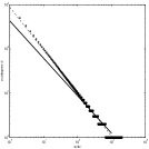
Figure 1: Out-degree $d$ vs. rank $r$. The $\star$’s are 2000 data points obtained from the relation (10) in text. The heavy solid line of slope $-0.85$ is the fitting to these data. Dash line is the fitting to the data of out-degree greater than 1, with slope $-0.97$.

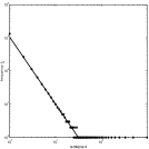
Figure 2: Frequency vs. out-degree $d$, following Fig. 1. The $\star$’s are data calculated with relation (3) in text. The heavy solid line is the fitting to data of out-degrees less than 33. The number of discarded data in the linear fitting is 26, only 1.3% of the total data.

Figure 3: The cascade of spike-like disturbance of steady state Internet toward large or small out-degree directions.

References

- (1) Faloutsos, M., Faloutsos, P. and Faloutsos, C.: On Power-Law Relationships of the Internet Topology, SIGCOMM’99, Cambridge, MA. http://www.cs.ucr.edu/ michalis/papers.html
- (2) Leland, W.E., Taqqu, M.S., Willinger, W. and Wilson, D.V.: On the self-similar nature of ethernet traffic. IEEE Transactions on Networking, 2(1):1-15, February 1994.
- (3) Paxson, V. and Floyd, S.: Wide-area traffic: The failure of Poisson modeling. IEEE/ACM Transactions in Networking, 3(3):226-244, June 1995
- (4) Willinger, W. and Paxson, V,: Where Mathematics meets the Internet. In Notices of the American Mathematical Society, 45(8), pp.961-970, Sept. 1998
- (5) Willinger, W., Paxson, V. and Taqqu, M.S.: Self-similarity and heavy-tails: Structure modeling of network traffic. In A Practical Guide to Heavy Tails: Statistics; Techniques and Applications, 1998. Adler, R., Feldman, R. and Taqqu, M.S., editors, Birkhauser