Slicing of Constraint Logic Programs

Abstract

Abstract. Slicing is a program analysis technique originally developed for imperative languages. It facilitates understanding of data flow and debugging.

This paper discusses slicing of Constraint Logic Programs. Constraint Logic Programming (CLP) is an emerging software technology with a growing number of applications. Data flow in constraint programs is not explicit, and for this reason the concepts of slice and the slicing techniques of imperative languages are not directly applicable.

This paper formulates declarative notions of slice suitable for CLP. They provide a basis for defining slicing techniques (both dynamic and static) based on variable sharing. The techniques are further extended by using groundness information.

A prototype dynamic slicer of CLP programs implementing the presented ideas is briefly described together with the results of some slicing experiments.

1 Introduction

This paper discusses slicing of Constraint Logic Programs. Constraint Logic Programming (CLP) (see e.g. [13]) is an emerging software technology with growing number of applications. Data flow in constraint programs is not explicit, and for this reason the concept of a slice and the slicing techniques of imperative languages are not directly applicable. Also, implicit data flow makes the understanding of program behaviour rather difficult. Thus program analysis tools explaining data flow to the user could be of great practical importance. This paper presents a prototype tool based on the slice concept applied to CLP.

Intuitively a program slice with respect to a specific variable at some program point contains all those parts of the program that may affect the value of the variable (backward slice) or may be affected by the value of the variable (forward slice). Slicing algorithms can be classified according to whether they only use statically available information (static slicing), or compute those statements which influence the value of a variable occurrence for a specific program input (dynamic slice). The slice provides a focus for analysis of the origin of the computed values of the variable in question. In the context of CLP the intuition remains the same, but the concept of slice requires precise definition since the nature of CLP computations is different from the nature of imperative computing.

Slicing techniques for logic programs have been discussed in [5, 14, 19]. CLP extends logic programming with constraints. This is a substantial extension and the slicing of CLP program has, to our knowledge, not yet been addressed by other authors. Novel contributions presented in this paper are:

• A precise formulation of the slicing problem for CLP programs. We first define a concept of slice for a set of constraints, which is then used to define slices of derivation trees, representing states of CLP computations. Then we define slices of a program in terms of the slices of its derivation trees.

• Slicing techniques for CLP. We present slicing techniques that make it possible to construct slices according to the definitions. The techniques are based on a simple analysis of variable sharing and groundness.

• A prototype dynamic slicer. A tool implementing the proposed techniques and some experiments with its use are briefly described.

The precisely defined concepts of slice gives a solid foundation for development of slicing techniques. The prototype tool, including some visualisation facilities, helps the user in better understanding of the program and in (manual) search for errors. Integration of this tool with more advanced debuggers is a topic of future work.

The paper is organized as follows. Section 2 outlines some basic concepts which are then used in Section 3 to formulate the problem of slicing. Section 4 presents and justifies a declarative formalization of CLP slicing, based on a notion of dependency relation. Section 5 discusses a dynamic backward slicing technique, and the use of directionality information for reducing the size of slices. Our prototype tool is described in Section 6, together with results of some experiments. Section 7 then discusses relations to other work. Finally in Section 8 we present our conclusions and suggestions for future work.

2 Constraint Logic Programs

The cornerstone of Constraint Logic Programming (CLP) [9, 13] is the notion of constraint. Constraints are formulae constructed with some constraint predicates with a predefined interpretation. A typical example of a constraint is a linear arithmetic equation or inequality with rational coefficients where the constraint predicate used is equality interpreted over rational numbers, e.g. $X-Y=1$. The variables of a constraint range over the domain of interpretation. A valuation of a set $S$ of variables is a mapping $\theta$ from $S$ to the interpretation domain. A set of constraints $C$ is satisfiable if there exists a valuation $\theta$ for the set of variables occurring in $C$, such that $\theta(C)$ holds in the constraint domain.

A constraint logic program is a set of clauses of the form $h:-b_{1},...,b_{n}$, $n\geq 0$ , where $h,b_{1},...,b_{n}$ are atomic formulae. The predicates used to construct $b_{1},...,b_{n}$ are either constraint predicates or other predicates (sometimes called defined predicates). The predicate of $h$ is a defined predicate. A goal is a clause without $h$. This syntax extends logic programs with the possibility of including constraints into the clauses.

Example 1

In the following constraint program the equality constraint and symbols of arithmetic operations are interpreted over the domain of rational numbers. This simple example is chosen to simplify the forthcoming illustration of slicing concepts and techniques. The constraints are distinguished by the curly brackets $\{\}$.

p(X,Y,Z):- {X-Y=1}, q(X,Y), r(Z).
q(U,V):- {U+V=3}.
r(42).

Slicing refers to computations. Abstractly, a computation can be seen as construction of a tree, from renamed instances of clauses. We explain briefly the idea discussed formally in [3].

Intuitively, a clause $c$ can be seen as a tree with root $h$ head and leaves $b_{1},...,b_{n}$ body atoms. If the predicate of $b_{i}$ appears in the head of a clause $c^{\prime}$ then a renamed copy $c^{\prime\prime}$ of $c^{\prime}$ can be composed with $c$ by attaching the head of $c^{\prime\prime}$ to $b_{i}$. This implicitly adds equality constraints for the corresponding arguments of the atoms. This process can be repeated for the leaves of the resulting tree. More formally this is captured by the following notion. A skeleton for a program $P$ is a labeled ordered tree with the root labeled by a goal clause and with the nodes labeled by (renamed) clauses of the program; some leaves may instead be labeled ”?” in which case they are called incomplete nodes. Each non-leaf node has as many children as the non-constraint atoms of its body. The head predicate of the $i$-th child of a node is the same as the predicate of the $i$-th non-constraint body atom of the clause labeling the node.

For a given skeleton $S$ the set $C(S)$ of constraints, which will be called the set of constraints of $S$, consists of :

• the constraints of all clauses labeling the nodes of $S$

• all equations $\vec{x}=\vec{y}$ where $\vec{x}$ are the arguments of the $i$-th body atom of the clause labeling a node $n$ of $S$, and $\vec{y}$ are the arguments of the head atom of the clause labeling the $i$-th child of $n$. (No equation is created if the $i$-th child of $n$ is an incomplete node).

A derivation tree for a program $P$ is a skeleton for $P$ whose set of constraints is satisfiable. If the skeleton is complete (i.e. it has no incomplete node) the derivation tree is called a proof tree. Figure 1 shows a complete skeleton tree for the program in Example 1.

Figure 1: A skeleton for the CLP program of Example 1.

The set of constraints of this skeleton is: $C(S)=\{X-Y=1,X=U,Y=V,U+V=3,Z=42\}$ and it is satisfiable. Thus the skeleton is a proof tree.

For the presentation of the slicing techniques we need to refer to program positions and to derivation tree positions. A slice is defined with respect to some particular occurrence of a variable (in a program or derivation tree), and positions are used to identify these ocurrences. Positions also identify arguments of the atomic formulae and their subterms.

To define the notion of position we assume that some standard way of enumeration of the nodes of any given tree $T$ is adopted. The indices of the nodes of $T$ are called positions of $T$ and the set of all positions is denoted $Pos(T)$. Each position determines a unique subtree of $T$. On the other hand, $T$ may have several identical subtrees $T_{0}$ at different positions.

This notation extends also for atomic formulae and terms, where the positions determine unique subterms. A position of a term such that the corresponding subterm is a variable will be called a variable position. We extend the adopted way of enumeration to clauses and programs; a program position is an index in this enumeration that identifies an atomic formula or a term in a clause of the program.

A single clause may be treated as a one-clause program. As discussed above, a derivation tree has its nodes labeled by renamed variants of program clauses. By a derivation tree position of a derivation tree $T$ we mean a pair $(i_{1},i_{2})$, where $i_{1}$ is a position of the skeleton of $T$ and $i_{2}$ is a position of the clause labeling node $i_{1}$ in $T$. The set of all tree positions of a derivation tree $T$ will be denoted by $Pos(T)$.

Recall that each label of a derivation tree $T$ is a variant of a program clause, or of a goal. Therefore the positions of $T$ can be mapped in a natural way into the corresponding program positions.

Similary, each occurrence of a variable $X$ in $C(T)$ (the constraint set of $T$) originates from a variable position of $X$ in $T$. Thus variable positions of $T$ can be linked to the related constraints of $C(T)$.

Let $\cal P$ be a set of positions of $T$, and $\Psi_{T}({\cal P})$ the set of all variables that appear in the terms on positions in $\cal P$. In this way $\cal P$ identifies the subset $C_{\cal P}$ of $C(T)$ consisting of all constraints including variables in $\Psi_{T}(\cal P)$.

Example 2

Consider the derivation tree of Figure 1.
Let $\cal(P)=\{$ derivation tree positions of the atom $q(X,Y)\}\subseteq Pos(T).$
Then $\Psi_{T}{\cal(P)}=\{X,Y\}$ and $C_{\cal P}=\{X-Y=1,X=U,Y=V\}.$

3 The Slicing Problem

Given a variable $X$ in a CLP program we would like to find a fragment of the program that may affect the value of $X$. This is rather imprecise, hence our objective is to formalize this intuition. We first define the notion of a slice of a satisfiable set of constraints. A variable $X$ in a derivation tree $T$ has its valuations [9, 13] restricted by the set of constraints of $T$ (which is satisfiable), so our second task will be to define a slice of a derivation tree, and finally a slice of a program (see Figure 2).

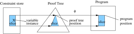
Figure 2: A slice of a constraint set, a proof tree and a program.

Let $C$ be a set of constraints. Intuitively we would like to remove all constraints of the set that do not restrict the valuation of a given variable. The binding of a variable $X$ to a value $v$ is said to be a solution of $C$ with respect to $X$ iff there exists a valuation $\nu$ such that $\nu(X)=v$ and $\nu$ satisfies $C$. The set of all solutions of $C$ with respect to $X$ will be denoted by $Sol(X,C)$.

Definition 1

A slice of a satisfiable constraint set $C$ with respect to $X$ is a subset $S\subseteq C$ such that $Sol(X,S)=Sol(X,C)$.

In other words the set of all solutions of a slice $S$ of $C$ with respect to $X$ is equal to the set of all solutions of $C$ with respect to $X$. Definition 1 gives implicitly a notion of minimal slice: it is a slice $S$ of $C$ such that if we further reduce $S$ to $S^{\prime}$, then $Sol(X,S^{\prime})$ is different from $Sol(X,C)$. Notice that the whole set $C$ is a slice of itself, and that the definition does not provide any hint about how to find a minimal slice. The problem of finding minimal slices may be undecidable in general, since satisfiability may be undecidable. So reasoning about minimality of the constructed slices seems only be possible in very restricted cases, and for some specific constraint domains. Our general technique is domain independent but we show in Section 5 how the groundness information ( which may be provided by a specific constraint solver) can be used to reduce the size of the slices constructed by the general technique.

We now formulate the slicing problem for derivation trees. A derivation tree $T$ is a skeleton with a set of constraints $C(T)$. The variables of $C(T)$ originate from positions of $T$. Let $\cal P$ be a set of positions of $T$, i.e. ${\cal P}\subseteq Pos(T)$. Then $\Psi({\cal P})$ identifies the variables of $C(T)$ with occurrences originating from positions in $\cal P$. We denote by $C_{\cal P}$ the set of all constraints of $C(T)$ that include these variables.

Definition 2

A slice of a derivation tree $T$ with respect to a variable position of $X$ is any subset $\cal P$ of the positions of $T$ such that $C_{\cal P}$ is a slice of $C(T)$ with respect to $X$.

The intuition reflected by this definition is that the constraints connected with the positions of the tree not included in a slice do not influence restrictions on the valuation of $X$ imposed by the tree. We formalize this by referring to the formal notion of the slice of a set of constraints. Notice that any superset of a slice is also a slice.

Finally we define the notion of a CLP program slice with respect to a variable position. We notice that every position of a derivation tree $T$ is a (renamed) copy of a program position or of a goal position. This provides a natural map $\Phi_{T}$ of the positions of $T$ into program positions and goal positions. Corresponding to this definition of $\Phi_{T}$, for a program position $q$ the set $\Phi^{-1}_{T}(q)$ contains those proof tree positions such that if $r\in\Phi^{-1}_{T}(q)$ then $\Phi_{T}(r)=q$.

Definition 3

A slice of a CLP program $P$ with respect to a program position $q$ is any set $S$ of positions of $P$ such that for every derivation tree $T$ whenever its position $r$ is in $\Phi_{T}^{-1}(q),$ there exists a slice $Q$ of $T$ with respect to $r$ such that $\Phi_{T}(Q)\subseteq S$.

This means that for any derivation tree position $r$, such that $\Phi_{T}(r)=q$, and program slice $S$ with respect to $q$, the value of the variable in $r$ can only be influenced by variants of the program positions in $S$.

4 Dependency-based slicing

The formal definitions of the previous section make it possible to state precisely our objective, which is automatic construction of slices.

Our formulation defines slicing of a CLP program in terms of the slicing of sets of constraints. Generally it is undecidable whether a subset of a set of constraints is a slice. This section presents a rather straightforward sufficient condition for this. We provide here a “syntactic” approach to slicing constraint stores, proof trees and programs. The propositions follow easily from the definitions and will be stated without proof. More details can be found in the technical report [16].

4.1 Slicing sets of constraints

We use variable sharing between constraints as a basis for slicing sets of constraints. Let $C$ be a set of constraints, and $vars(C)$ the set of all variables occurring in the constraints in $C$. Let $X,Y$ be variables in $vars(C)$. $X$ is said to depend explicitly on $Y$ iff both occur in a constraint $c$ in $C$. Notice that the explicit dependency relation is symmetric and reflexive but need not be transitive.

Definition 4

A dependency relation on $vars(C)$ is the transitive closure of the explicit dependency relation.

The dependency relation on $C$ will be denoted by $dep_{C}$. Notice that $dep_{C}$ is an equivalence relation on $vars(C)$. We map any equivalence class $[X]_{dep_{C}}$ to the subset $C_{X}$ of $C$ that consists of all constraints that include variables in $[X]_{dep}$. Then $C_{X}$ is a slice of $C$ (see [16]).

Example 3

For the set of constraints of Example 1 the dependency relation has two equivalence classes: $\{X,Y,U,V\}$ and $\{Z\}$ and gives the following slice of $C$ with respect to $X$:

$$C_{X}=\{X-Y=1,\ X=U,\ Y=V,\ U+V=3\}$$

4.2 Slicing of derivation trees

We defined the concept of slice for a derivation tree by referring to the notion of slice of a set of constraints. To construct slices of derivation trees we introduce a dependency relation on the positions of a derivation tree. We now define a direct dependency relation $\sim_{T}$ on $Pos(T)$. It can be related to the dependency relation on $vars(C(T))$ [16] and hence can be used for slicing $T$.

Definition 5

Let $T$ be a derivation tree. The direct dependency relation $\sim_{T}$ on $Pos(T)$ is defined as follows:
$\alpha\sim_{T}\beta$ iff one of the following conditions holds:

1. $\alpha$ and $\beta$ are positions in an occurrence of a clause constraint (constraint edge).

2. $\alpha$ and $\beta$ are positions in a node equation (transition edge).

3. $\alpha$ and $\beta$ are positions in an occurrence of a term (functor edge).

4. $\alpha$ and $\beta$ share a variable (local edge).

Observe that the relation is both reflexive and symmetric. The transitive closure $\sim^{*}_{T}$ of the direct dependency relation will be called the dependency relation on $Pos(T)$. So $\sim^{*}_{T}$ is an equivalence relation.

Proposition 1

Let $T$ be a proof tree and let $\alpha$ be a variable position of $T$. Then $[\alpha]_{\sim^{*}_{T}}$ is a slice of $T$ with respect to $\alpha$.

4.3 Slicing of CLP programs

This section defines a dependency relation on the positions of the program and then makes use of it in constructing program slices. Recall that each position of a derivation tree $T$ “originates” from a position of the selected program $P$. This is formally captured by the map $\Phi:Pos(T)\rightarrow Pos(P)$. The dependency relation $\sim_{P}$ on $Pos(P)$ we are going to define should reflect dependency relations in all proof trees of $P$. More precisely, whenever $\alpha\sim_{T}\beta$ in some tree $T$ we would also like to have $\Phi(\alpha)\sim_{P}\Phi(\beta)$.

Definition 6

Let $P$ be a CLP program. The direct dependency relation $\sim_{P}$ on $Pos(P)$ is defined as follows: $\alpha\sim_{P}\beta$ iff at least one of the following conditions holds:

1. $\alpha$ and $\beta$ are positions of the same constraint (constraint edge).

2. $\alpha$ is a position of the head atom of a clause $c$ and $\beta$ is a position of a body atom of a clause $d$ and both atoms have the same predicate symbol (transition edge).

3. $\alpha$ and $\beta$ belong to the same argument of a function (functor edge).

4. $\alpha$ and $\beta$ are in the same clause and have a common variable (local edge).

The dependency relation of a program can be represented as a graph.

Figure 3: Program dependence represented in graphical form and the backward slice with respect to Z in p(X,Y,Z))

Comparing the definitions of $\sim_{T}$ and $\sim_{P}$ one can check that whenever $\alpha\sim_{T}\beta$ in some tree $T$ of $P$ then $\Phi(\alpha)\sim_{P}\Phi(\beta)$ as well. Consequently, for any proof tree $T$ $(\alpha\sim_{T}^{*}\beta)\Rightarrow\Phi(\alpha)\sim_{P}^{*}\Phi(\beta)$. The transitive closure $\sim_{P}^{*}$ is an equivalence relation on $Pos(P)$. The following result shows how $\sim_{P}^{*}$ can be used for the slicing of $P$.

Proposition 2

Let $P$ be a CLP program and let $\beta$ be a position of $P$. Then $[\beta]_{\sim_{P}^{*}}$ is a slice of $P$ with respect to $\beta$.

Figure 3 shows the program dependences and a backward slice of the program in Example 1 with respect to $Z$ in $p(X,Y,Z)$. For the program in Example 1 $\sim_{P}^{*}$ has two equivalence classes. One of them includes all occurrences of $Z$ and the occurrence of the constant 42. The other consists of the remaining positions.

Definition 6 with Proposition 2 give a method for constructing program slices without referring to proof trees. Thus, we obtain a static slicing technique for CLP. The mapping $\Phi$ was introduced to argue about correctness of this technique. These results also confirm the correctness of the slicing algorithm in [5] since a logic program can be viewed as a constraint logic program.
The proposition shows that the concept of dependency relation on program positions provides a sufficient condition for slicing a CLP program. However, the slice obtained may be quite large, sometimes it may even include the whole constraint store.

We propose two ways for addressing this problem. On one hand, improvement is possible if we handle the so called “calling context problem”[7] which appears when the same predicate is called from two different clauses. As we explained in [16] it is possible to adapt to CLP the solution proposed by Horwitz et. al [7] for procedural languages. Another way of reducing the size of slices is to infer and to take into account information about proliferation of ground instantiations during the execution of the program. A directional dynamic slicing technique based on this idea is presented in the next section.

5 Dynamic directional slicing

All the dependency relations discussed so far were symmetric. Intuitively, for a constraint $c(X,Y)$ a restriction imposed on valuations of $X$ usually influences admissible valuations of $Y$ and vice versa. However if $c(X,Y)$ belongs to a satisfiable constraint set $C$ and some other constraints of $C$ make $X$ ground then the slice of $C$ with respect to $X$ need not include $c(X,Y)$. For example, if $C=\{X+1=0,Y>X\}$ is interpreted on the integer domain then $\{X+1=0\}$ is a slice of $C$ with respect to $X$. This slice can be constructed by using information about groundness of variables occurring in the dependency graph.

This section shows how to use groundness information in derivation tree slicing, that is in dynamic slicing of CLP programs. It extends to CLP the ideas of dynamic slicing for logic programs presented in [5]. In our approach groundness is captured by adding directionality information to dependency graphs. The directed graphs show the propagation of ground data during the execution of CLP programs, and these graphs can then be used to produce more precise slices. The groundness information will be collected during the computation that constructs the derivation tree to be sliced. The proposed concepts are also applicable to the case of static slicing, where the groundness information has to be inferred by static analysis of the program. This is however not discussed in this paper.

5.1 Groundness Annotations

Groundness information associated with a derivation tree will be expressed as an annotation of its positions. The annotation classifies the positions of a derivation tree or the positions of the CLP program. The positions are classified as inherited (marked with $\downarrow$), synthesized ($\uparrow$) and dual ($\updownarrow$). An annotation is partial if some positions are dual. Formally speaking, an annotation is a mapping $\mu$ from the positions into the set $\{\downarrow,\uparrow,\updownarrow\}$ [3].

The intended meaning of the annotation is as follows. An inherited position is a position which is ground at time of calling, that is when the equation involving this position is first created during the construction of the derivation tree. A synthesized positions is a position which is ground at success, that is when the subtree having the position in its root label is completed in the computation process. The dual positions of a proof tree are those for which no groundness information is given, including those which are ground neither at call nor at success.

The annotations will be collected during the execution of the program. Alternatively, they may be inferred with some straightforward inference rules discussed in [16].

We now introduce the following auxiliary terminology relevant to the annotated positions of a CLP program. The inherited positions of the head atoms and the synthesized positions of the body atoms are called input positions. Similarly, the synthesized positions of the head atoms and inherited positions of the body atoms are called output positions. Note that dual positions are not strictly classified as input or output ones. Alternatively, if we say that a position is annotated as an output we mean that it is annotated as inherited provided it is a position in a body atom, or annotated as synthesized if it is a position of the head of a clause.

Example 4

Consider the following CLP program:

1. p(X,Y) :- r(X), q(X,Y).
2. r(3).
3. q(U,V) :- {U+V = 5}.

The corresponding annotated proof tree for the goal $p(X,Y)$ is presented in Figure 4, where the actual positions have been replaced by I (the input positions) and by O (the output positions):

Figure 4: The annotated proof tree for Example 5

The annotation reflects groundness propagation during the computation, as discussed below. The variables $X$ and $Y$ of $p(X,Y)$ are annotated as output, since they are ground at success of $p$, and $p(X,Y)$ is a head atom. For the same reason the argument of the fact $r(3)$ in node 2 is annotated as output. The variable $U$ in the first argument of the predicate $q(U,V)$ in node 3 is ground at call, so it is annotated as input, while $V$ is ground at success of $q$ so it is annotated as output.

In a CLP program groundness of a position depends generally on the used constraint solver. Monitoring the execution, also in this case, we are able to annotate certain positions as inputs or outputs. For example the $indomain(X)$ constraint of CHIP instantiates $X$ to a value in its domain, so that $X$ is an input position. Rational solvers can usually solve linear equations. For example in the rational constraint $Y=2*X+Z$, $X$ can be annotated input if $Y$ an $Z$ are output.

5.2 Directional slicing of derivation trees

Having input/output information for positions of a derivation tree, we then add directions to its dependence graph. The following definition describes how it can be achieved.

Definition 7

Directed Dependency Graph of a Proof Tree
Let $T$ be a proof tree, $T_{G}=(TreePos(T),\sim_{T})$ its proof tree dependence graph, then the directed dependence graph of $T(P)$ can be defined as:
$T_{DG}=(TreePos(T),\rightarrow_{T})$, where:

• $\alpha\rightarrow_{T(G)}\beta$ if $\alpha\sim_{T(G)}\beta$ is a transition edge, $\alpha$ is an output position and $\beta$ is an input position

• $\alpha\rightarrow_{T(G)}\beta$ if $\alpha\sim_{T(G)}\beta$ is a local edge, $\alpha$ is an input position and $\beta$ is an output position

• $\alpha\rightarrow_{T(G)}\beta$ and $\beta\rightarrow_{T(G)}\alpha$ in every other case when $\alpha\sim_{T(G)}\beta$

From the definition of $\rightarrow_{T(G)}$ assuming correctness of the annotation we find that if $\alpha$ is a position of $X$ in $T$ and it is annotated as input or as output then $C(T)$ binds $X$ to a single value. This value is determined by the constraints connected with those positions that are in the set $\{\beta|{\beta}\rightarrow^{*}_{T(G)}\alpha\}$. Thus we have:

Proposition 3

$\{\beta|{\beta}\rightarrow^{*}_{T(G)}\alpha\}$ is a slice of $T$ with respect to $\alpha$.

These slices are usually more precise than in the case when the groundness information is not used.

The concept of directed dependency graph can be extended to programs and used for static slicing. This requires good methods for static groundness analysis to infer annotations for program positions. Some suggestions for that can be found in [16].

6 A Prototype Implementation

We developed a prototype in SICStus Prolog for dynamic backward slicing of constraint logic programs written in SICStus. The tool handles a realistic subset of Prolog, including constructs such as cut, if-then and or. The inputs of the slicing system are: the source code, a test case (a goal) and (after the execution) the execution traces given by the Prolog interpreter. From this information the Directed Proof Tree Dependence Graph (Definition 7) may be constructed. The following three types of slice algorithms were implemented (see Figure 5):

1. Proof tree slice
   In this case the user chooses an argument position of the created Proof Tree, and the slice is constructed with respect to this proof tree position using the Directed Proof Tree Dependency Graph (see Definition 7). This kind of slice is useful when the user is interested in the data dependences of the Proof Tree.

2. Dynamic slice
   This case is very similar to 1, but the constructed slice of the Proof Tree is mapped back to the program. This is the classic dynamic slice approach [12], as in the case of procedural languages. So this slice provides a slice of the program.

3. Program position slice
   In this case the user selects a program position. The system provides all instances of this program position in the Proof Tree, creates the proof tree slice for every instance, then the union of these slices are constructed and mapped back to the program. So this algorithm also provides a slice of the program, which shows all dependences of a program position for a given test case.

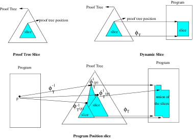
Figure 5: Proof Tree, Dynamic and Program Position Slice.

A graphical interface draws the proof tree (see Figure 7), marked with different colored nodes that are in the Proof tree slice, and in the case of a dynamic slice and program position slice the corresponding slice of the program is highlighted. The label of the nodes identify the nodes of the proof tree including the name of the predicate and the annotation of its arguments.

In the implementation we applied a very simple annotation technique: the inherited positions were those which were ground at the time of calling, while synthesized positions were those which were ground at success. This method provides precise annotation, because we continuously extract information from the actual state of the constraint store. However, in the current implementation slicing can only be done on argument positions. If an argument includes several variables it is not possible to distinguish between them, which makes the constructed slice ”less precise” (compared to the minimal slice). So, our aim is to improve the existing implementation, extend it to variable positions.

In the present version of the tool the sliced proof tree corresponds to the first success branch of the SLD tree. As the proof tree slice definition is quite general, there is no real difficulty in applying the technique to all success branches of SLD tree. The extension to failure branches is discussed in [6]. Currently we are working on an implementation of these extensions.

Systematic slicing experiments were performed on a number of constraint logic programs (written in SICSTus Prolog). Each of them was executed with a number of test inputs to collect data about the relative size of a slice with respect to the proof tree, depending on the choice of the position. The selected application programs [9, 13] had different language structures (use of cut, or, if-then, databases, compound constraint), and were of different size.

The summarized data of the test results on proof tree slicing is listed in Table 1. The comparison of the three kind of slices with respect to the number of nodes are shown in Figure 6.

	PROGRAM	NUMBER OF	NUMBER OF	NUM. OF COMP-	AVERAGE	SIZE OF	AVERAGE	SIZE OF
		CLAUSES	TEST CASES	UTED SLICES	THE PROOF	TREE	SLICES
					NODE	ARG. POS.	NODE	ARG.POS.
1	LIGHTMEAL	11	1	17	9	15	44.64 %	41.17 %
2	CIRC	5	2	139	33.35	54.09	35.14 %	54.44 %
3	SUM	6	4	626	80.26	120.77	30.46 %	49.34 %
4	FIB	4	6	1349	399.57	533.51	7.56 %	8.53 %
5	SCHEDULING	20	1	575	134	390	51.21 %	71.66 %
6	PUZZLE	30	2	1363	227.57	607.82	19.05 %	14.93 %

Table 1: Proof Tree Slice

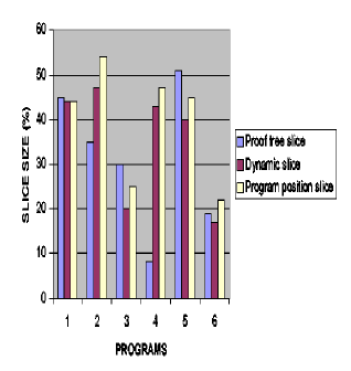
Figure 6: Comparison of the Proof Tree Slice, Dynamic Slice and the Program Position Slice.

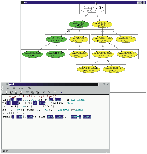
Figure 7: Displayed program and proof tree slices.

It should be mentioned that the average slice size (in percent) in these experiments had no correlation with the size of the program. The average slice size was $32\%$ of the number of executed nodes and $40\%$ of the executed argument positions.

The intended application of our slicing method is to support debugging of constraint programs. A bug in a program shows up as a symptom during the execution of the program on some input. This means that in some computation step (i.e. in some derivation tree) a variable of the program is bound in a way that does not conform to user expectations. A slice of the derivation tree with respect to this occurrence of the variable can be mapped into the text of the program and will identify a part of the program where the undesired binding was produced. This would provide a focus for debugging, whatever is the debugging technique used. Intersection of the slices produced for different runs of the buggy program may further narrow the focus.

In particular, our slicing technique can be combined with Shapiro’s algorithmic debugging [15], designed originally for logic programs. As shown in [11] the slice of a derivation tree of a logic program may reduce the number of queries of algorithmic debugger. This technique can also be applied to the case of algorithmic debugging of CLP programs discussed in [19].

7 Related Work

Program slicing has been widely studied for imperative programs [4, 10, 8, 12, 7]. To our knowledge only a few papers have dealt with the problem of slicing logic programs, and slicing of constraint logic programs has not been investigated till now.

We provided a theoretical basis for the slicing of proof trees and programs starting from a semantic definition of the constraint set dependence. This applies as well to the special case of logic programs (the Herbrand domain). In particular it justifies the slicing technique of Gyimóthy and Paakki [5] developed to reduce the number of queries for algorithmic debugger and makes it possible to extend the latter to the general case of CLP. The directional slicing of Section 5 is an extension of this technique to the general case of CLP.

Schoening and Ducassé [14] proposed a backward slicing algorithm for Prolog which produces executable slices. For a target Prolog program they defined a slicing criterion which consists of a goal of $P$ and a set of argument positions $P_{a}$, along with a slice $S$ as a reduced and executable program derived from $P$. An executable slice is usually less precise but it may be used for additional test runs. Hence the objectives of their work are somewhat different from ours, and their algorithm is applicable to a limited subset of Prolog programs.

In [19] Zhao et al defined some static and dynamic slices of concurrent logic programs called literal dependence nets. They presented a new program representation called the argument dependence net for concurrent logic programs to produce static slices at the argument level. There are some similarities between our slicing techniques and Zhao’s methods, since we also rely on some dependency relations. However, the focus of our work has been on CLP not on concurrent logic programs, and our main aim has been a declarative formulation of the slicing problem whic provides a clear reference basis for proving the correctness of the proposed slicing methods.

The results of the ESPRIT Project DiSCiPl [2] show the importance of visualisation in the debugging of constraint programs. Our tool provides a rudimentary visualisation of the sliced proof tree. It was pointed out by Deransart and Aillaud [1] that abstraction techniques are needed in the visualisation of the search space. Program position slicing, if applied to all branches of the SLD-tree, provides yet another abstraction of the search space.

8 Conclusions

The paper offers a precise declarative formulation of the slicing problem for CLP. It also gives a solid reference basis for deriving various techniques of slicing CLP programs in general and for logic programs treated as a special case. This technique was illustrated by deriving the directional data flow slicing technique for CLP, which is an extension of [5] applied to CLP. As a side effect, the latter, which was presented in somewhat pragmatic setting, obtains a theoretical justification.

The paper presents also a prototype slicing tool using this technique. The experiments with the tool show that the obtained slices were quite precise in some cases, and on average provided a substantial reduction of the program.

The future work will focus on the application of slicing techniques to constraint programs debugging. Two aspects being considered. Firstly, in the manual debugging of CLP programs it is necessary to support user with a tool that facilitates the understanding of the program. We believe that a future version of our slicer equipped with suitable visualisation features could be very suitable for this purpose. Secondly, the slicing of a derivation tree can often reduce the number of queries in algorithmic debugging of logic programs [15]. (The algorithmic debugging technique has been extended to CLP [17]).

As a first step in this direction we are going to integrate our CLP slicing tool with the IDTS algorithmic debugger [11], originally developed for pure logic programs.

Acknowledgments

The work of the first and second authors was supported by the grants OTKA T52721 and IKTA 8/99.

References

- [1] P. Deransart and C. Aillaud: Towards a Language for CLP Choice-tree Visualisation, In: P. Deransart, M. Hermenegildo, and J. Małuszyński, (editors), Analysis and Visualization Tools for Constraint Programming, LNCS. Springer Verlag, 2000 (to appear).
- [2] P. Deransart, M. Hermenegildo, and J. Małuszyński, (editors), Analysis and Visualization Tools for Constraint Programming, LNCS. Springer Verlag, 2000 (to appear).
- [3] P. Deransart and J. Małuszyński: A grammatical view of logic programming. The MIT Press 1993.
- [4] T. Gyimóthy, Á. Beszédes and I. Forgács: An Efficient Relevant Slicing Method for Debugging. In Proceedings of 7th European Software Engineering Conference (ESEC’99), LNCS 1687 Springer Verlag, pages 303-322, Toulouse, France, September 1999.
- [5] T. Gyimóthy and J. Paakki: Static Slicing of Logic Programs. In Proceedings of Second International Workshop on Automated and Algorithmic Debugging (AADEBUG’95), pages 85-105, Saint Malo, France, May 1995.
- [6] Harmath L., Szilágyi Gy., Gyimóthy, T., Csirik J.: Dynamic Slicing of Logic Programs. Program Analysis and verification, Fenno-Ugric Symposium (FUSST’99), pages 101-113, Tallin, Estonia 1999.
- [7] S. Horwitz, T. Reps and D. Binkley: Interprocedural Slicing Using Dependence Graphs. In Proceedings of ACM Transactions on Programming Languages and Systems 12, pages 26-61, 1990.
- [8] S. Horwitz and T. Reps: The Use of Program Dependence Graphs in Software Engineering. In Proceedings of the Fourteenth International Conference on Software Engineering , pages 392-411, Melbourne, Australia, May 1992.
- [9] J.Jaffar and M.J.Maher: Constraint logic programming: A survey. The Journal of Logic Programming 19/20:503-582, 1994.
- [10] M. Kamkar and P. Fritzson: Evaluation of Program Slicing tools. In 2nd International Workshop on Automated and Algorithmic Debugging (AADEBUG’95) , pages 51-69, Saint Malo, France, May 1995.
- [11] G. Kókai, L Harmath, T. Gyimóthy: Algorithmic Debugging and Testing of Prolog Programs, In Proceedings of the Fourteenth International Conference on Logic Programming, Eighth Workshop on Logic Programming Environments (ICLP’97), pages 14-21, Leuven, Belgium, September 1997.
- [12] B. Korel and J. Rilling: Application of Dynamic Slicing in Program Debugging. In Proceedings of the Third International Workshop on Automatic Debugging (AADEBUG ’97), Linköping, pages 43-59, Sweden, May 1997.
- [13] K. Marriott and P.J. Stuckey: Programming with Constraints. An Introduction. The MIT Press, 1998
- [14] S. Schoening and M. Ducassé: A Backward Slicing Algorithm for Prolog. In Proceedings of Third International Static Analysis Symposium SAS’96, LNCS 1145, 317-331, Springer-Verlag 1996.
- [15] E. Shapiro: Algorithmic Debugging. The MIT Press, 1983.
- [16] Gy. Szilágyi, T. Gyimóthy, J. Maluszyński: Slicing of Constraint Logic Programs. Technical Report, Linköping University Electronic Press 1998/020, www.ep.liu.se/ea/cis/1998/002.
- [17] A. Tessier and G. Fèrrand. Declarative Diagnosis in the CLP Scheme, In: P. Deransart, M. Hermenegildo, and J. Małuszyński, (editors), Analysis and Visualization Tools for Constraint Programming, LNCS. Springer Verlag, 2000 (to appear).
- [18] F. Tip: A survey of Program Slicing Techniques. Journal of Programming Languauges, Vol.3., No.3, pages 121-189, September, 1995.
- [19] J. Zhao, J. Cheng and K. Ushijima: Slicing Concurrent Logic Programs. In Proceedings of Second Fuji International Workshop on Functional and Logic Programming, pages 143-162, 1997.