Kima – an Automated Error Correction System for Concurrent Logic Programs

Abstract

We have implemented Kima, an automated error correction system for concurrent logic programs. Kima corrects near-misses such as wrong variable occurrences in the absence of explicit declarations of program properties.

Strong moding/typing and constraint-based analysis are turning to play fundamental roles in debugging concurrent logic programs as well as in establishing the consistency of communication protocols and data types. Mode/type analysis of Moded Flat GHC is a constraint satisfaction problem with many simple mode/type constraints, and can be solved efficiently. We proposed a simple and efficient technique which, given a non-well-moded/typed program, diagnoses the “reasons” of inconsistency by finding minimal inconsistent subsets of mode/type constraints. Since each constraint keeps track of the symbol occurrence in the program, a minimal subset also tells possible sources of program errors.

Kima realizes automated correction by replacing symbol occurrences around the possible sources and recalculating modes and types of the rewritten programs systematically. As long as bugs are near-misses, Kima proposes a rather small number of alternatives that include an intended program. Search space is kept small because the minimal subset confines possible sources of errors in advance. This paper presents the basic algorithm and various optimization techniques implemented in Kima, and then discusses its effectiveness based on quantitative experiments.

1 Introduction

In our previous work [1], we proposed a framework of automated debugging of program errors based on static, constraint-based program analysis in the absence of programmers’ declarations. The framework was then implemented in Kima, an automated error correction system for concurrent logic programs, which featured several improvements to make the system more practical and efficient.

The mechanism of error correction in Kima is based on the mode and type system of Moded Flat GHC [9][10]. Moded Flat GHC is a concurrent logic (and consequently, a concurrent constraint) language with a constraint-based mode system designed by one of the authors. Languages equipped with strong typing or strong moding enable the detection of type/mode errors by checking or reconstructing types or modes. The best-known framework for type reconstruction is the Hindley-Milner type system [4], which allows us to solve a set of type constraints obtained from program text efficiently as a unification problem.

Similarly, the mode system of Moded Flat GHC allows us to solve a set of mode constraints obtained from program text as a constraint satisfaction problem. Mode reconstruction statically determines the read/write capabilities of variable occurrences and establishes the consistency of communication protocols between concurrent processes [10]. As we will see later, types in Moded Flat GHC also can be reconstructed using a similar (and simpler) technique.

When a concurrent logic program contains bugs, it is very likely that mode constraints obtained from the erroneous symbol occurrences are incompatible with the other constraints. We have proposed an efficient algorithm that finds a minimal inconsistent subset of mode constraints from an inconsistent (multi)set of constraints [3]. Since each constraint keeps track of the symbol occurrence(s) in the program that imposed the constraint, a minimal subset tells possible sources (i.e., symbol occurrences) of mode errors.

Using the information of possible locations of bugs, automated correction is attempted basically by generate-and-test search, namely the generation of possible rewritings and the computation of their principal mode and type. Search space is kept small because the locations of bugs have been limited to small regions of program text.

A significant feature of our framework is that it is applicable to a fragment of a program such as a set of predicate definitions in a particular module. That is, our framework is quite effective, for example, in the situation where a program is not completely constructed. This is due to the fact that the multiset of mode constraints imposed by a program usually has redundancy. Redundancy comes from two reasons:

1. A non-trivial program contains conditional branches or nondeterministic choices. In (concurrent) logic languages, they are expressed as a set of rewrite rules (i.e., program clauses) that may impose the same mode constraints on the same predicate.

2. A non-trivial program contains predicates that are called from more than one place, some of which may be recursive calls. The same mode constraint may be imposed by different calls.

Although the framework is quite general, whether it is practical or not may depend on the choice of a language. Kima corrects wrong occurrences of variable symbols in a KL1 [8] program assuming strong moding and typing of Moded Flat GHC. KL1 is designed based on Flat GHC that is not equipped with strong moding/typing, but the debugging of KL1 programs turns out to benefit from moding and typing. Furthermore, its compiler KLIC provides a nice platform for our experiments [2]. We have obtained promising results from our experiments with the assistance of other syntactical constraints (Sect. 5).

2 Strong Moding and Typing in Concurrent Logic Programming

We outline the mode system of Moded Flat GHC. The readers are referred to [10] and [7] for details.

In concurrent logic programming, modes play a fundamental role in establishing the safety of a program in terms of the consistency of communication protocols. The mode system of Moded Flat GHC gives a polarity structure (that determines the information flow of each part of data structures created during execution) to the arguments of predicates that determine the behavior of goals. A mode expresses this polarity structure, which is represented as a mapping from the set of paths to the two-valued codomain $\{\hbox{\it in\/},\hbox{\it out\/}\}$. Paths here are strings of pairs, of the form $\langle{\hbox{\it symbol}},\allowbreak{\hbox{\it arg}}\rangle$, of predicate/function symbols and argument positions, and are used to specify possible positions in data structures. Formally, the set $P_{\it Term}$ of paths for terms and the set $P_{\it Atom}$ of paths for atomic formulae are defined using disjoint union as:

$$P_{\it Term}=(\sum_{f\in{\it Fun}}N_{f})^{*}\,,\;P_{\it Atom}=(\sum_{p\in{\it Pred}}N_{p})\times P_{\it Term}\enspace\,,$$

where Fun/Pred are the sets of function/predicate symbols, and $N_{f}$/$N_{p}$ are the sets of possible argument positions (numbered from 1) for the symbols $f$/$p$. The disjoint union operator $\sum$ means:

$$\sum_{f\in{\it Fun}}\!\!\!\!N_{f}=\{\langle{f},\allowbreak{i}\rangle~{}|~{}f\in{\it Fun},~{}i\in N_{f}\}\,\,.$$

The purpose of mode analysis is to find the set of all modes (each of type $P_{\it Atom}\rightarrow\{\hbox{\it in\/},\hbox{\it out\/}\}$) under which every piece of communication is cooperative. Such a mode is called a well-moding. Intuitively, in means the inlet of information and out means the outlet of information. A program does not usually define a unique well-moding but has many of them. So the purpose of mode analysis is to compute the set of all well-modings in the form of a principal (i.e., most general) mode. Principal modes can be expressed naturally by mode graphs, as described later in this section.

Given a mode $m$, we define a submode $m/p$, namely $m$ viewed at the path $p$, as a function satisfying $(m/p)(q)=m(pq)$. We also define IN and OUT as submodes returning in and out, respectively, for any path. An overline ‘$\,\overline{\hbox{\vrule height=4.0pt,depth=3.5pt,width=0.0pt}~{}~{}}\,$’ inverts the polarity of a mode, a submode, or a mode value.

A Flat GHC program is a set of clauses of the form $h\mathrel{\!\hbox{\tt:-}}G\mathrel{\hbox{\tt|}}B$, where $h$ is an atomic formula and $G$ and $B$ are multisets of atomic formulae. Mode constraints imposed by a clause $h\mathrel{\!\hbox{\tt:-}}G\mathrel{\hbox{\tt|}}B$ are summarized in Fig. 1. All rules here embody the assumption that every piece of communication is cooperative. Rule (BU) numbers unification body goals because the mode system allows different body unification goals to have different modes. This is a special case of mode polymorphism that can be introduced into other predicates as well [3], but in this paper we will not consider general mode polymorphism because whether to have polymorphism is independent of the essence of this work.

•    (HF) $m(p)=\hbox{\it in\/}$, for a function symbol occurring in $h$ at $p$. (HV) $m/p=\hbox{\it IN\/}$, for a variable symbol occurring more than once in $h$ at $p$ and somewhere else. (GV) If some variable occurs both in $h$ at $p$ and in $G$ at $p^{\prime}$,
  $\forall q\mathbin{\in}P_{\it Term}\bigl{(}m(p^{\prime}q)=\hbox{\it in\/}\Rightarrow m(pq)=\hbox{\it in\/}\bigr{)}$. (BU) $m/\langle{\hbox{\tt=}_{k}},\allowbreak{1}\rangle=\overline{m/\langle{\hbox{\tt=}_{k}},\allowbreak{2}\rangle}$, for a unification body goal $\hbox{\tt=}_{k}$. (BF) $m(p)=\hbox{\it in\/}$, for a function symbol occurring in $B$ at $p$. (BV) Let $v$ be a variable occurring exactly $n\,(\geq 1)$ times in $h$ and $B$ at $p_{1},\ldots,p_{n}$, of which the occurrences in $h$ are at $p_{1},\ldots,p_{k}$ ($k\geq 0$). Then $$\cases{{\cal R}\bigl{(}\{m/p_{1},\ldots,m/p_{n}\}\bigr{)},&if $k=0$;\cr{\cal R}\bigl{(}\{\overline{m/p_{1}},m/p_{k+1},\ldots,m/p_{n}\}\bigr{)},&if $k>0$;\cr}$$ where the unary predicate ${\cal R}$ over finite multisets of submodes represents “cooperative communication” between paths and is defined as $${\cal R}(S)\mathrel{\mathop{=}\limits^{\rm def}}\forall q\mathbin{\in}P_{\it Term}\,\exists s\mathbin{\in}S\bigl{(}s(q)=\hbox{\it out\/}\,\land\,\forall s^{\prime}\mathbin{\in}S\mskip-4.0mu\mathrel{\backslash}\mskip-4.0mu\!\{s\}\,\bigl{(}s^{\prime}(q)=\hbox{\it in\/}\bigr{)}\bigr{)}.$$   

Figure 1: Mode constraints imposed by a program clause $h\mathrel{\!\hbox{\tt:-}}G\mathrel{\hbox{\tt|}}B$ or a goal clause $\mathrel{\!\hbox{\tt:-}}B$.

The cost of mode analysis is almost proportional to the program size for the following reason. Mode analysis proceeds by merging many simple mode graphs representing individual mode constraints. For example, the resulting mode graph of the append program (cf. Appendix) is shown in Fig. 2. The mode graphs of very large programs are, in general, much wider than that of the append program but are not much deeper, which is to say most nodes can be reachable within several steps from the root. The cost of merging one mode constraint with a mode graph is almost proportional to the depth of the mode graph, but does not depend on the width of the graph [7]. So the total cost is proportional to the number of constraints that in turn is proportional to the program size.

•      

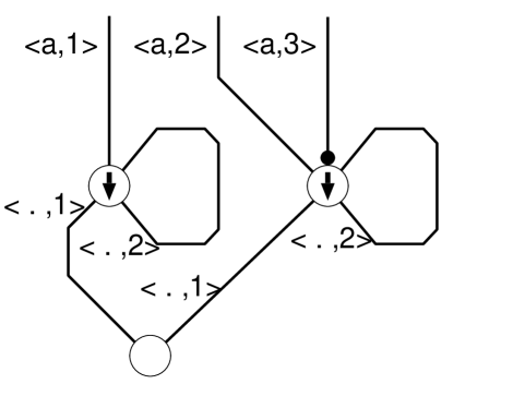
Figure 2: The mode graph of an append program. “a” stands for append; “.” stands for list constructor; and the downward arrow means the mode value in. The mode information of the toplevel predicate and unification goals is omitted.

A type system for concurrent logic programming can be introduced by classifying the set Fun of function symbols into mutually disjoint sets $F_{1},\ldots,F_{n}$. A type here is a function from $P_{\it Atom}$ to the set $\{F_{1},\ldots,F_{n}\}$. Like principal modes, principal types can be computed by unification over feature graphs. Constraints on a well-typing $\tau$ are summarized in Fig.  3. The choice of a family of sets $F_{1},\ldots,F_{n}$ is somewhat arbitrary. This is why moding is more fundamental than typing in concurrent logic programming.

•    $({\rm HBF}_{\tau})$ $\tau(p)=F_{i}$, for a function symbol occurring at $p$ in $h$ or $B$. $({\rm HBV}_{\tau})$ $\tau/p=\tau/p^{\prime}$, for a variable occurring both at $p$ and $p^{\prime}$ in $h$ or $B$. $({\rm GV}_{\tau})$ $\forall q\mathbin{\in}P_{\it Term}\bigl{(}m(p^{\prime}q)=\hbox{\it in\/}\Rightarrow\tau(pq)=\tau(p^{\prime}q)\bigr{)}$, for a variable occurring both at $p$ in $h$ and at $p^{\prime}$ in $G$. $({\rm BU}_{\tau})$ $\tau/\langle{\hbox{\tt=}_{k}},\allowbreak{1}\rangle=\tau/\langle{\hbox{\tt=}_{k}},\allowbreak{2}\rangle$, for a unification body goal $\hbox{\tt=}_{k}$.   

Figure 3: Type constraints imposed by a program clause $h\mathrel{\!\hbox{\tt:-}}G\mathrel{\hbox{\tt|}}B$ or a goal clause $\mathrel{\!\hbox{\tt:-}}B$.

The type system employed by Kima classifies function symbols into six disjoint sets — integers, floating-point numbers, strings, vectors, lists and functor structures, and prohibits any two of them from sharing the same path. Although this is a heuristic classification based on the fact that these different types do not simultaneously appear in the same path in most programs, an experiment proves that it is beneficial both to the power of error detection and to the quality of error correction, as we will see in Sect. 6.

3 Identifying Program Errors

When a concurrent logic program contains an error, it is very likely (though not always the case) that its communication protocols become inconsistent and the set of its mode constraints becomes unsatisfiable. A wrong symbol occurring at some path is likely to impose a mode constraint inconsistent with constraints representing the intended specification.

Then, suspicious symbols can be located by computing a minimal inconsistent subset of mode constraints, because the minimal inconsistent subset must include at least one wrong constraint, and each constraint is imposed on certain symbol occurrences in a clause (see the moding rules in Fig. 1). Type constraints can be used in the same way to locate type errors.

A minimal inconsistent subset can be computed efficiently using a simple algorithm shown in Fig. 4 . Let $C=\{c_{1},\dots,c_{n}\}$ be a multiset of constraints. The algorithm finds a single minimal inconsistent subset $S$ from $C$ when $C$ is inconsistent. When $C$ is consistent, the algorithm terminates with $S=\{\}$. $false$ is a self-inconsistent constraint used as a sentinel.

•    $c_{n+1}\leftarrow false;\;$ $S\leftarrow\{\};$ while $S$ is consistent do $D\leftarrow S;\;i\leftarrow 0;$ while $D$ is consistent do $i\leftarrow i+1;\;D\leftarrow D\cup\{c_{i}\}$ end while; $S\leftarrow S\cup\{c_{i}\}$ end while; if $i=n+1$ then $S\leftarrow\{\}$ fi   

Figure 4: Algorithm for computing a minimal inconsistent subset

The readers are referred to [3] for a proof of the minimality of $S$, as well as various extensions of the algorithm. Note that the algorithm can be readily extended to finding multiple bugs at once. That is, once we have found a minimal subset covering a bug, we can reapply the algorithm to the rest of the constraints.

Our experiment shows that the average size of minimal inconsistent subsets is rather small, and the subsets containing more than 10 elements are scarcely found. The size of minimal subsets turns out to be independent of the total number of constraints, and most inconsistencies can be explained by constraints imposed by a small range of program text. This is due to the redundancy of mode and type constraints.

4 Automated Debugging

Constraints that are considered wrong may be corrected by

• replacing the symbol occurrences that imposed those constraints by other symbols, or

• when the suspected symbols are variables, by making them have more occurrences elsewhere (cf. Rule (BV) of Fig. 1).

When some symbol occurrence has been rewritten to another symbol by mistake, there exists a symbol with less occurrences than intended and a symbol with more occurrences. A minimal inconsistent subset includes either (or both) of them.

Kima focuses on programs with a small number of errors in variables. This may sound restrictive, but concurrent logic programs have quite flat syntactic structures (compared with other languages) and instead make heavy use of variables. Our experience tells that a majority of simple program errors arises from the erroneous use of variables, for which the support of a static mode and type system and debugging tools are invaluable.

This technique is applicable also to mutations between a constant and a variable symbol, because mode and type constraints are imposed also on constant symbols. Even mutations between constant symbols could be corrected by type constraints. However, when considering replacement by a constant symbol, Kima must determine its value. It is difficult for the current version of Kima to determine the value based on modes and types only. Mutations of function symbols (other than constant symbols) can also be located but their correction is difficult because search space will expand too much. Mutations of predicate symbols cannot be corrected by the current framework.

4.1 Basic Algorithm

An algorithm for automated correction is basically a search procedure whose initial state is the erroneous program, whose operations are the rewriting of the occurrences of variables, and whose final states are well-moded/typed programs.

The algorithm in Fig. 5 finds a set $S$ of alternative solutions. The main procedure of the algorithm is iterative-deepening search up to the maximum depth MAX which is to be given by a user. $\delta$ represents the current depth.

•    Compute a minimal inconsistent subset of mode/type constraints; Extract suspicious variable symbols from the subset; $\delta\leftarrow 1;\;\;S\leftarrow\{\};$ while MAX $\geq\delta$ do for each way of rewriting $\delta$ symbol occurrences do if the rewritten program becomes well-moded/typed then Add the way of rewriting to $S$ fi end for; $\delta\leftarrow\delta+1$ end while   

Figure 5: The basic algorithm for automated error correction

Since checking modes and types of a rewritten program requires the cost proportional to the program size (Sect. 2), this algorithm takes time in proportion to the program size. However, inconsistency usually occurs within a small region of program text (Sect. 3). A large performance improvement will therefore be achieved by analyzing those constraints imposed by the suspected predicates and its closely related predicates before the whole constraints.

4.2 Grouping Errors

As we mentioned in Sect. 3, multiple minimal inconsistent subsets may independently be found, and some of them may indicate the same clause as the source of errors. The clause may be indicated by subsets of modes, types, or both. Modes and types express different properties of a program and detect different kinds of errors. To use them together makes two improvements; one is that more errors can be detected; the other is that errors can be located more precisely. Kima collects minimal inconsistent subsets indicating the same clause (as in Fig. 6), and makes them belong to the same group which plays the role of a unit of searching alternatives against errors.

Figure 6: Grouping minimal inconsistent subsets

Depth-$\delta$ search of alternatives is carried out independently for each group. It is possible to reduce computation time by checking whether a certain rewriting can possibly dissolve inconsistencies of all minimal inconsistent subsets in a group before actually computing modes and types, which is called Quick-check. This is effective because when some symbol occurrence is rewritten, even if the change is small, mode and type analyses may reanalyse the whole program. To put it more precisely, Quick-check of a rewriting is to check if, for all minimal inconsistent subsets in a group, there exists a variable indicated as a possible source of mode/type errors such that the given rewriting will result in:

• replacing an occurrence of the indicated variable by a different variable, or

• making more occurrences of the indicated variable elsewhere.

When multiple groups are found, mode and type analyses are performed with the constraints imposed by one of the groups and consistent part. The consistent part is the set of all constraints which do not belong to any minimal inconsistent subset. Therefore, not all constraints imposed by the whole program text are considered in error correction. Kima employs such an algorithm so that the search of alternatives for one group may not be influenced by that for another group. Alternatives found for a group do not always include an intended one.

5 Constraints Other Than Modes and Types

5.1 Prioritizing Alternatives

Kima searches alternative solutions using mode and type information, but unfortunately, multiple alternatives are found in many cases. Kima refines the quality of its output by prioritizing alternatives using two Heuristic Rules:

Heuristic Rule 1.

It is less likely that a variable occurs

1. only once in a clause (singleton occurrence),

2. two or more times in a clause head,

3. three or more times in the head and/or the body of a clause, or

4. two or more times as arguments of the same body goal.

Heuristic Rule 2.

It is less likely that a list and its elements are of the same type, that is, it is less likely that a variable occurs both in some path $p$ and in the path of its elements $p\langle{\hbox{\tt.}},\allowbreak{1}\rangle$.

Since such variable occurrences as in Heuristic Rules 1.1, 1.2 and 1.3 impose mode constraints IN or OUT (Sect. 2) that are stroger than in and out, we could replace Heuristic Rules 1.1-1.3 by a unified rule on constraint strength; A solution with weaker mode constraints is more likely to be an intended one. In general, stronger mode/type constraints make a program less generic, and the execution of the program more likely to end in failure. Therefore it is reasonable to insist that the constraint imposed on a program should be as weak as possible.

Heuristic Rules 1.1 and 1.3 are justified also in the sense that logical variables are used for one-to-one communication more frequently than for one-to-many or one-to-zero communication. A logical variable used for one-to-one communication occurs either exactly twice in the clause body or exactly once in the clause head and once in the clause body. Such a body goal as in Heuristic Rule 1.4 either receives duplicate data from another goal or communicates with itself, which are both unlikely.

For Heuristic Rule 2, let $\alpha$ be a type variable and $list(\alpha)$ be the list type whose elements are of type $\alpha$. Then the rule is equivalent to saying that constraint $\alpha=list(\alpha)$ imposes a strong type constraint on $\alpha$ and is therefore unlikely.

Kima prioritizes multiple alternatives by imposing certain penalty points on unlikely symbol occurrences. An alternative with a lower penalty point has a higher priority.

5.2 Reinforcing Detection Power

The objective of Kima is to debug a program in the absence of explicit declarations. To enhance the power of the error detection with implicit modes and types, Kima employed the following Detection Rules:

Detection Rule 1.

1. A variable which occurs in a clause guard must occur also in the head of the clause.

2. The same variable must not occur on both sides of a unification body goal (partial occur-check).

Detection Rule 2.

The name of a singleton variable must begin with an underscore “-”.

The both Detection Rules are optional and can be used selectively in Kima.

Violation of Detection Rule 1.1 means disappearance of a guard goal after normalization [10], while violation of Detection Rule 1.2 means failure of normalization. Detection Rule 2 is identical to requesting the declaration of variables that impose strong mode constraints. Detection Rule 2 is effective because a logical variable in a correct program is likely to occur twice in a clause (i.e., for one-to-one communication), in which case a variable will turn into a singleton if either occurrence is missing.

The source of an error detected by Detection Rules is a variable symbol in a certain clause, and is found independently of minimal inconsistent subsets of mode and type constraints. Kima uniformly deals with a variable symbol detected by Detection Rules by considering it as a minimal inconsistent subset with one element, and groups it with other subsets.

5.3 Optimizing Search of Alternatives

Kima employs two optimization techniques other than Quick-check. The two techniques are based on prioritizing and Detection Rules stated in Sect. 5.1 and 5.2, and reduce the number of mode and type analyses in generate-and-test search. The algorithm shown in Fig. 7 finds a set $S$ of alternatives that have higher priorities than the given priority $P$. Steps related to grouping process (Sect. 4.2) are omitted.

•    Compute a minimal inconsistent subset of mode/type constraints; Extract suspicious variable symbols from the subset; Detect clauses and variable symbols infringing Detection Rules; $\delta\leftarrow 1;\;\;S\leftarrow\{\};$ while MAX $\geq\delta$ do for each way of rewriting $\delta$ symbol occurrences which has a higher priority than $P$ w.r.t. Heuristic Rule 1 do if the rewritten program follows Detection Rules then if the rewritten program becomes well-moded/typed then if the rewriting is unlikely w.r.t. Heuristic Rule 2 then lower the priority of the rewriting fi; Add the way of rewriting to $S$ with its priority fi fi end for; $\delta\leftarrow\delta+1$ end while   

Figure 7: The optimized algorithm for automated error correction

In generate-and-test search, the test by Detection Rules is cheaper than mode and type analyses, because, when particular (suspected) clauses are rewritten, the clauses that are not rewritten do not have to be checked with Detection Rules again. In contrast, mode and type analyses may need recalculation of the whole program (Sect. 4.2).

Prioritizing with Heuristic Rule 1 involves only suspected clauses, and is cheaper than mode and type analyses. Prioritizing with Heuristic Rule 2 needs type analysis, and is performed after the check of well-typedness (i.e., type reconstruction).

For a quicksort program containing two wrong variable occurrences in the same clause (Example 3 in Appendix), the above optimization improved the response time of computing highest-priority alternatives from 25.9 seconds to 10.2 seconds on the KLIC system running on Sun Ultra 30 (248 MHz) + 128 MB of memory.

6 Experiments

We discuss the effectiveness of our technique based on experiments. We investigated how many of programs with a few errors are detected as erroneous by Kima, how many alternatives it proposes for erroneous programs, and how many “plausible” programs there are in the neighborhood of a correct (original) program.

First, we systematically generated near-misses (each with one wrong occurrence of a variable) of three programs and examined how many of them could be detected, whether automated correction reported an intended program, and how many alternatives were reported. Table 1 shows the results . Here, we did not consider the mutation of a variable occurrence to the variable whose name began with “-”. We used only the definitions of predicates, that is, we did not use the constraints that might be imposed by the caller of these programs. Of course, the caller information, if available, would enhance the quality of correction as well as the redundancy of constraints.

Table 1: Single-error detection and correction

Program	Analysis	Level	Priori-	Total	Dete-	Proposed Alternatives
			tizing	cases	cted	1	2	3	4	5	6	$\mathord{\geq}7$
append	mode only	0	no	58	36	1	3	8	3	6	5	10
	type only	0	no	58	0	0	0	0	0	0	0	0
	mode & type	0	no	58	36	1	3	8	3	6	5	10
	mode & type	0	yes	58	36	27	9	0	0	0	0	0
	mode & type	1	yes	58	40	29	11	0	0	0	0	0
	mode & type	2	yes	58	58	39	19	0	0	0	0	0
fibonacci	mode only	0	no	118	57	10	7	9	6	4	1	20
	type only	0	no	118	47	0	0	4	20	0	18	5
	mode & type	0	no	118	72	18	13	2	15	9	0	15
	mode & type	0	yes	118	72	54	11	1	6	0	0	0
	mode & type	1	yes	118	88	68	12	7	0	1	0	0
	mode & type	2	yes	118	99	71	18	8	0	2	0	0
quicksort	mode only	0	no	300	177	34	70	1	12	19	0	41
	type only	0	no	300	106	0	2	12	40	0	32	20
	mode & type	0	no	300	221	49	76	8	59	0	9	20
	mode & type	0	yes	300	221	164	41	16	0	0	0	0
	mode & type	1	yes	300	236	175	61	0	0	0	0	0
	mode & type	2	yes	300	286	199	84	2	1	0	0	0

The programs we used are list concatenation (append), the generator of a Fibonacci sequence, and quicksort. They are admittedly simple but the aim of the experiment is to investigate the fundamental power of our technique based on exhaustive experiments. Further, for the reason discussed in Sect. 4.1, we strongly expect that the total program size does not make much difference in the quality of automated debugging.

The column “Level” indicates detection levels. Under detection level 0, only mode and/or type information was used; under detection level 1, Detection Rule 1 was used in addition; and under detection level 2, Detection Rules 1 and 2 were used together. The two Detection Rules raised the average detection rate from 69.1% (329/476) to 93.1% (443/476).

A row with “yes” in the column “Prioritizing” shows the number of proposed alternatives with the highest priority, which includes an intended alternative in most cases. The number of proposed alternatives under prioritizing was usually 1 or quite small.

Second, we investigated the error detection rate for programs with two and three mutated variable occurrences in the same clause. Errors of this kind are looked on as depth-2 and depth-3 errors in the same group, respectively, and their correct alternatives can be obtained by depth-2 and depth-3 search. Table 2 shows the results. Note that the mutation of variable occurrences does not always cause errors. For example, certain mutations make a program equivalent to the original as we will see later.

Table 2: The error detection rate for the programs with N mutations

Program	N	Level	Total	Detected	Detection
			cases	cases	rate (%)
append	2	0	1200	937	78.1
	2	1	1200	1004	83.7
	2	2	1200	1141	95.1
	3	0	16980	14597	86.0
	3	1	16980	15411	90.8
	3	2	16980	16674	98.2
fibonacci	2	0	4668	3982	85.3
	2	1	4668	4330	92.8
	2	2	4668	4489	96.2
	3	0	133045	125300	94.2
	3	1	133045	130325	97.9
	3	2	133045	131810	99.1
quicksort	2	0	12102	11263	93.1
	2	1	12102	11460	94.7
	2	2	12102	12005	99.2
	3	0	337455	330769	98.0
	3	1	337455	332416	98.5
	3	2	337455	336943	99.8

When multiple errors existed in some clause of a program, the program was detected as long as at least one of the errors caused inconsistency. So the detection rate for multiple errors was higher than that for a single error. The detection rate with Detection Rules 1 and 2 was above 95% in every case.

Third, we explored the number of “plausible” programs. Plausible programs are programs that have the same or higher priority than the original among the programs with N mutations on variable occurrences in the same clause for a certain N. The result is shown in Table 3. We considered the mutations to the variable whose name began with “-”. In the column “Plausible programs”, programs that were

1. equivalent up to renaming of variables and

2. equivalent up to switching of arguments of calls to commutative built-in predicates such as unification

were counted as one program.

Table 3: The number of plausible programs among the programs with N mutations

Program	N	Total	Plausible
		cases	programs
append	1	58	0
	2	1200	7
	3	16980	14
	4	167842	29
fibonacci	1	118	11
	2	4668	66
	3	133045	309
quicksort	1	300	9
	2	12102	33
	3	337455	76

From Table 3 we see that the number of plausible programs did not increase explosively. This can be explained by the fact that the ways of placing variable symbols which make a program well-moded/typed are extremely limited compared to arbitrary ways of placing.

Now we focus on the number of proposed alternatives under prioritizing. Suppose, for example, a program contains two errors on variable occurrences and depth-2 search is performed. In this case, up to four occurrences may be rewritten from the original, in which the rewritings with N=4 will be the majority. However, since two of the four rewritings have already been done by the given erroneous program, only part of the rewritings where N is up to 4 is generated. The total number of rewritings generated actually is very close to the number of rewritings with N=2.

Among the plausible programs, the percentage of programs that neither diverge or fail depends on the original program and its expected input. In the case of quicksort, about fifty percent of plausible programs were programs that neither diverge or fail. We note that, of these programs, few were considered meaningful, that is, few programs were such that all operations contribute to the result of computation.

7 An Example — Fibonacci sequence

As an example, we consider the generator of a Fibonacci sequence with one error:

•    1:  $R_{1}$ : $\hbox{\tt fib(Max,\lower 3.0pt\hbox{-}\nobreak,~{}~{}N2,Ns0)}\mathrel{\!\hbox{\tt:-}}\hbox{\tt N2 >Max}\mathrel{\hbox{\tt|}}\hbox{\tt Ns0}\!\mathrel{\hbox{\tt=}}\!_{1}\hbox{\tt[]}\mathpunct{\hbox{\tt.}}$ 2:  $R_{2}$ : $\hbox{\tt fib(Max,N1,N2,Ns0)}\mathrel{\!\hbox{\tt:-}}\hbox{\tt N2=<Max}\mathrel{\hbox{\tt|}}$ 3:            $\hbox{\tt N1}\!\mathrel{\hbox{\tt=}}\!_{2}\hbox{\tt[N2|Ns1]}\hbox{\tt N3:=N1+N2}\hbox{\tt fib(Max,N2,N3,Ns1)}\mathpunct{\hbox{\tt.}}$   (the unification in the line 3 should be $\hbox{\tt Ns0}\!\mathrel{\hbox{\tt=}}\!_{2}\hbox{\tt[N2|Ns1]}$)   

The algorithm shown in Sect. 3 computes three independenet minimal inconsistent subsets; two on modes and one on types. Here, we do not consider Detection Rule 2 (though it can detect the variable Ns0 in the clause head of $R_{2}$ as an error).

Minimal inconsistent subset 1 (on modes):

Mode constraint			Rule	Source symbol
$m(\langle{\hbox{\tt=}_{1}},\allowbreak{2}\rangle)$	$=$	in	(BF)	“[]” in $R_{1}$
$m/\langle{\hbox{\tt=}_{1}},\allowbreak{1}\rangle$	$=$	$m/\langle{\hbox{\tt fib}},\allowbreak{4}\rangle$	(BV)	Ns0 in $R_{1}$
$m/\langle{\hbox{\tt=}_{1}},\allowbreak{2}\rangle$	$=$	$\overline{m/\langle{\hbox{\tt=}_{1}},\allowbreak{1}\rangle}$	(BU)	$\hbox{\tt=}_{1}$ in $R_{1}$
$m(\langle{\hbox{\tt fib}},\allowbreak{4}\rangle)$	$=$	IN	(BV)	Ns0 in $R_{2}$

Minimal inconsistent subset 2 (on modes):

Mode constraint			Rule	Source symbol
$m(\langle{\hbox{\tt=}_{2}},\allowbreak{2}\rangle)$	$=$	in	(BF)	“.” in $R_{2}$
$m/\langle{\hbox{\tt=}_{2}},\allowbreak{2}\rangle$	$=$	$\overline{m/\langle{\hbox{\tt=}_{2}},\allowbreak{1}\rangle}$	(BU)	$\hbox{\tt=}_{2}$ in $R_{2}$
$m(\langle{\hbox{\tt=}_{2}},\allowbreak{1}\rangle)$	$=$	IN	(BV)	N1 in $R_{2}$

Minimal inconsistent subset 3 (on types):

Type constraint			Rule	Source symbol
$\tau/\langle{\hbox{\tt fib}},\allowbreak{2}\rangle$	$=$	$\tau/\langle{\hbox{\tt:=}},\allowbreak{2}\rangle\langle{\hbox{\tt+}},\allowbreak{1}\rangle$	(${\rm HBV}_{\tau}$)	N1 in $R_{2}$
$\tau(\langle{\hbox{\tt=}_{2}},\allowbreak{2}\rangle)$	$=$	list type	(${\rm HBF}_{\tau}$)	“.” in $R_{2}$
$\tau/\langle{\hbox{\tt fib}},\allowbreak{2}\rangle$	$=$	$\tau/\langle{\hbox{\tt=}_{2}},\allowbreak{1}\rangle$	(${\rm HBV}_{\tau}$)	N1 in $R_{2}$
$\tau/\langle{\hbox{\tt=}_{2}},\allowbreak{2}\rangle$	$=$	$\tau/\langle{\hbox{\tt=}_{2}},\allowbreak{1}\rangle$	(${\rm BU}_{\tau}$)	$\hbox{\tt=}_{2}$ in $R_{2}$
$\tau(\langle{\hbox{\tt:=}},\allowbreak{2}\rangle\langle{\hbox{\tt+}},\allowbreak{1}\rangle)$	$=$	integer type	builtin	:= in $R_{2}$

These three subsets are classified into the same group because all of the subsets indicate the clause $R_{2}$. Suspected variable symbols are extracted as in the table below:

Clause	Variable symbol	Subset number
$R_{1}$	Ns0	1
$R_{2}$	Ns0	1
$R_{2}$	N1	2, 3

When depth-1 search is attempted, Quick-check detects that rewritings which increase or decrease the number of occurrences of Ns0 in $R_{1}$ need not be considered, because such changes may dissolve the subset 1 but neither the subset 2 nor 3. After all, the system finds that the only possible ways to dissolve all inconsistencies are either replacing Ns0 by N1 or vice versa in $R_{2}$. As the number of occurrences of Ns0 and N1 is four in total, only four ways of rewriting each variable occurrence need mode and type analyses. Without Quick-check, a great number of mode and type analyses would have to be done. In this example, Kima finally finds only one alternative, which is the program we have intended.

8 Related Work

Analysis of malfunctioning systems based on their intended logical specification has been studied in the field of artificial intelligence [5] and known as model-based diagnosis, which has some similarities with our work. However, the purpose of model-based diagnosis is to analyze the differences between intended and observed behaviors, while our system does not require that the intended behavior of a program be given as declarations.

Wand proposed an algorithm for diagnosing non-well-typed functional programs [11]. His approach was to extend the unification algorithm for type reconstruction to record which symbol occurrence imposed which constraint. In contrast, our framework is built outside any underlying framework of constraint solving. It does not incur any overhead for well-moded/typed programs or modify the constraint-solving algorithm.

Tenma’s system automatically corrects procedural programs under strong typing [6]. When a change is made on a certain software component, the system automatically replaces the components that do not adapt to the change by alternative components. Thus the purpose of the system is very different from Kima. Kima works in the situation where the locations of errors are entirely unknown, and it works at the program symbol level rather than the software component level.

9 Conclusions and Future Work

We have implemented Kima, a system which automatically corrects near-misses in a concurrent logic program. Kima does not have to be given explicit specifications of program properties.

Experiments showed that, in most cases, one or a few alternatives could be obtained from KL1 programs with a few wrong variable occurrences. This is indebted to theoretically or statistically endorsed heuristics as well as mode and type information. In the set of programs with a few mutated variable occurrences, programs that are both well-moded/typed and with higher priority turn out to be quite rare. Heuristic Rules and Detection Rules do not only improve detection power and the quality of alternatives but also optimizes the search of alternatives.

Specifications or declarations of program properties, if available, will achieve more advanced error correction. Our future plan is to let Kima accept instances of a pair of input and output constraints. Such instances play the role of mode and type specifications also.

Kima is itself written in KL1 language, and is now 4,500 lines long. The computation of minimal inconsistent subsets and the following depth-1 search for a program of 100 lines long is completed within several seconds. The example shown in Sect. 7 took not more than 0.1 seconds on the KLIC system running on Sun Ultra 30 (248 MHz) + 128 MB of memory.

Appendix: Usage of Kima

Example 1 – A single error

First, consider a list concatenation (append) program with one error:

•           $\mathrel{\!\hbox{\tt:-}}\hbox{\tt module test}\mathpunct{\hbox{\tt.}}$ $R_{1}$ : $\hbox{\tt append([],~{}~{}~{}~{}~{}Y,Z~{}~{})}\mathrel{\!\hbox{\tt:-}}\hbox{\tt true}\mathrel{\hbox{\tt|}}\hbox{\tt Y}\!\mathrel{\hbox{\tt=}}\!\hbox{\tt Z}\mathpunct{\hbox{\tt.}}$ $R_{2}$ : $\hbox{\tt append([A|Y],Y,Z0)}\mathrel{\!\hbox{\tt:-}}\hbox{\tt true}\mathrel{\hbox{\tt|}}\hbox{\tt Z0}\!\mathrel{\hbox{\tt=}}\!\hbox{\tt[A|Z]}\hbox{\tt,}\hbox{\tt append(X,Y,Z)}\mathpunct{\hbox{\tt.}}$ (The head of $R_{2}$ should have been append([A|X],Y,Z0))   

Suppose you want to obtain alternatives with up to priority 100 (i.e., very low priority), command line options should be given as:

•   

    % kima +p 100 append.kl1
  

    

Then, Kima presents six alternatives, all up to priority 3:

•   

      ================= Suspected Group 1 =================
             ------------- Priority 1 -------------
    append([A|X],Y,Z0):-true|Z0=[A|Z],append(X,Y,Z)
                            in test:append/3, clause No.2
             -----
    append([A|Y],X,Z0):-true|Z0=[A|Z],append(X,Y,Z)
                            in test:append/3, clause No.2
             -----
             ------------- Priority 2 -------------
    append([A|Y],Y,Z0):-true|Z0=[A|Z],append(Z0,Y,Z)
                            in test:append/3, clause No.2
             -----
             ------------- Priority 3 -------------
    append([A|Y],Y,Z0):-true|Z0=[A|Z],append(Y,Y,Z)
                            in test:append/3, clause No.2
             -----
    append([A|Y],Y,Z0):-true|Z0=[A|Z],append(A,Y,Z)
                            in test:append/3, clause No.2
             -----
    append([A|Y],Y,Z0):-true|Z0=[A|Z],append(Z,Y,Z)
                            in test:append/3, clause No.2
             -----
  

    

The two alternatives of priority 1 have the highest priority. Each alternative is separeted by “-----”. The first of the two alternatives with priority 1 is the intended one, while the second alternative turns out to be a program that merges two input lists by taking their elements alternately. That is, when append is invoked as append([1,2,3],[4,5,6],Out), the first alternative returns [1,2,3,4,5,6] and the second returns [1,4,2,5,3,6].

Next, let us compute minimal inconsistent subsets (MIS for short) and variable symbol occurrences infringing Detection Rules.

•   

    % kima +mis append.kl1
    < Minimal Inconsistent Subsets of *Mode* constraints >
    m/<(test:append)/3,1><cons,2> = IN
            imposed by the rule HV applied to the variable Y
            in test:append/3, clause No.2
    m/<(test:append)/3,1> = OUT
            imposed by the rule BV applied to the variable X
            in test:append/3, clause No.2
    -----
    < Minimal Inconsistent Subsets of *Type* constraints >
     --Constraints are consistent, and there is no MIS--
  
    < Violations of syntactic rules of the detection level 2 >
    singleton(X)
            in test:append/3, clause No.2
    -----
  

    

MISs of mode constraints are obtained first; those of types second. Multiple independent MISs can be computed at once, and each MIS is displayed with a separator “-----”. In this example, only one MIS on modes is found, while type constraints are consistent.

The MIS says that variables X and Y in the second clause of append are suspicious. Using this information, Kima searches alternatives either by increasing or by decreasing the occurrences of X and/or Y in the clause. In addition to MISs, the variable X is detected as an error by Detection Rule 2. Violations of Detection Rules are reported as follows:

Detection Rule 1.

1. A variable which occurs in a clause guard must occur also in the head of the clause: var-not-in-the-head(the variable)

2. The same variable must not occur on both sides of a unification body goal: not-pass-occur-check(the variable)

Detection Rule 2.

The name of a singleton variable must begin with an underscore “-”: singleton(the variable)

Example 2 – Independent errors

The second example is a program comb(n,r,Out) that generates the list of all length-$n$ 0-1 lists that contain exactly $r$ 1’s. (Hence the outer list contains ${}_{n}{\rm C}_{r}$ elements.) For example, comb(3,2,Out) returns the list
[[1,1,0],[1,0,1],[0,1,1]]. Below is the definition of comb with two errors:

•          $\mathrel{\!\hbox{\tt:-}}\hbox{\tt module probability}\mathpunct{\hbox{\tt.}}$ $R_{1}$: $\hbox{\tt comb(N,0,C)}\mathrel{\!\hbox{\tt:-}}\hbox{\tt true}\mathrel{\hbox{\tt|}}\hbox{\tt init\lower 3.0pt\hbox{-}\nobreak list(0,N,0,[],C0)}$,$\hbox{\tt C}\!\mathrel{\hbox{\tt=}}\!\hbox{\tt[C0]}\mathpunct{\hbox{\tt.}}$ $R_{2}$: $\hbox{\tt comb(N,N,C)}\mathrel{\!\hbox{\tt:-}}\hbox{\tt true}\mathrel{\hbox{\tt|}}\hbox{\tt init\lower 3.0pt\hbox{-}\nobreak list(0,N,1,[],C0)}$,$\hbox{\tt C}\!\mathrel{\hbox{\tt=}}\!\hbox{\tt[C0]}\mathpunct{\hbox{\tt.}}$ $R_{3}$: $\hbox{\tt comb(N,R,C)}\mathrel{\!\hbox{\tt:-}}\hbox{\tt~{}N>R}\mathrel{\hbox{\tt|}}$            N1:=N-1,R1:=R-1,comb(N1,R1,C0),cons-list(1,C0,CC0),            comb(N1,R,C1),cons-list(0,C1,CC1),$\hbox{\tt append(CC0,CC1,CC)}\mathpunct{\hbox{\tt.}}$  (The last invocation should have been append(CC0,CC1,C)) $R_{4}$: $\hbox{\tt init\lower 3.0pt\hbox{-}\nobreak list(N,Len,\lower 3.0pt\hbox{-}\nobreak,L0,L)}\mathrel{\!\hbox{\tt:-}}\hbox{\tt N=:=Len}\mathrel{\hbox{\tt|}}\hbox{\tt L0}\!\mathrel{\hbox{\tt=}}\!\hbox{\tt L}\mathpunct{\hbox{\tt.}}$ $R_{5}$: $\hbox{\tt init\lower 3.0pt\hbox{-}\nobreak list(N,Len,E,L0,L)}\mathrel{\!\hbox{\tt:-}}\hbox{\tt N~{}<~{}Len~{}}\mathrel{\hbox{\tt|}}$            $\hbox{\tt L1}\!\mathrel{\hbox{\tt=}}\!\hbox{\tt[E|L0]}$,N1:=N+1,$\hbox{\tt init\lower 3.0pt\hbox{-}\nobreak list(N1,Len,E,L1,L)}\mathpunct{\hbox{\tt.}}$ $R_{6}$: $\hbox{\tt cons\lower 3.0pt\hbox{-}\nobreak list(\lower 3.0pt\hbox{-}\nobreak,[],~{}~{}~{}~{}~{}~{}~{}L)}\mathrel{\!\hbox{\tt:-}}\hbox{\tt true}\mathrel{\hbox{\tt|}}\hbox{\tt L}\!\mathrel{\hbox{\tt=}}\!\hbox{\tt[]}\mathpunct{\hbox{\tt.}}$ $R_{7}$: $\hbox{\tt cons\lower 3.0pt\hbox{-}\nobreak list(A,[X|Xs],L)}\mathrel{\!\hbox{\tt:-}}\hbox{\tt true}\mathrel{\hbox{\tt|}}$            $\hbox{\tt L}\!\mathrel{\hbox{\tt=}}\!\hbox{\tt[[A|X]|L1]}$,$\hbox{\tt cons\lower 3.0pt\hbox{-}\nobreak list(A,XS,L1)}\mathpunct{\hbox{\tt.}}$  (The recursive call should have been cons-list(A,Xs,L1)) $R_{8}$: $\hbox{\tt append([],~{}~{}~{}~{}~{}Y,Z~{}~{})}\mathrel{\!\hbox{\tt:-}}\hbox{\tt true}\mathrel{\hbox{\tt|}}\hbox{\tt Y}\!\mathrel{\hbox{\tt=}}\!\hbox{\tt Z}\mathpunct{\hbox{\tt.}}$ $R_{9}$: $\hbox{\tt append([A|X],Y,Z0)}\mathrel{\!\hbox{\tt:-}}\hbox{\tt true}\mathrel{\hbox{\tt|}}\hbox{\tt Z0}\!\mathrel{\hbox{\tt=}}\!\hbox{\tt[A|Z]}$,$\hbox{\tt append(X,Y,Z)}\mathpunct{\hbox{\tt.}}$   

The default action of Kima is to perform depth-1 search of alternatives of the highest priority using modes, types, and Detection Rules.

•   

    % kima comb.kl1
     ================= Suspected Group 1 =================
            ------------- Priority 1 -------------
    comb(N,R,C):-N>R|
    N1:=N-1,R1:=R-1,comb(N1,R1,C0),cons_list(1,C0,CC0),
    comb(N1,R,C1),cons_list(0,C1,CC1),append(CC0,CC1,C)
                           in probability:comb/3, clause No.3
            -----
     ================= Suspected Group 2 =================
            ------------- Priority 1 -------------
    cons_list(A,[X|Xs],L):-true|L=[[A|X]|L1],cons_list(A,Xs,L1)
                           in probability:cons_list/3, clause No.2
            -----
  

    

There are two Suspected Groups. In this example, Kima first found multiple MISs. By analyzing the clauses indicated by the MISs, Kima concluded there were two independent groups. Kima performed depth-1 search of alternatives for each group, and finally succeeded in finding alternatives that really corrected the errors.

Example 3 – Multiple errors in the same group

Last, we consider a quicksort program with two errors in the same clause.

•           $\mathrel{\!\hbox{\tt:-}}\hbox{\tt module main}\mathpunct{\hbox{\tt.}}$ $R_{1}$ : $\hbox{\tt quicksort(Xs,Ys)}\mathrel{\!\hbox{\tt:-}}\hbox{\tt true}\mathrel{\hbox{\tt|}}\hbox{\tt qsort(Xs,Ys,[])}\mathpunct{\hbox{\tt.}}$ $R_{2}$ : $\hbox{\tt qsort([],~{}~{}~{}~{}~{}~{}~{}Ys0,Ys~{}~{})}\mathrel{\!\hbox{\tt:-}}\hbox{\tt true}\mathrel{\hbox{\tt|}}\hbox{\tt Ys}\!\mathrel{\hbox{\tt=}}\!\hbox{\tt Ys0}\mathpunct{\hbox{\tt.}}$ $R_{3}$ : $\hbox{\tt qsort([X|Xs],Ys0,Ys3)}\mathrel{\!\hbox{\tt:-}}\hbox{\tt true}\mathrel{\hbox{\tt|}}$             part(X,Xs,S,L),qsort(S,Ys0,Ys1),             $\hbox{\tt Ys2}\!\mathrel{\hbox{\tt=}}\!\hbox{\tt[X|Ys1]}\hbox{\tt,}\hbox{\tt qsort(L,Ys2,Ys3)}\mathpunct{\hbox{\tt.}}$  (The body unification goal should have been $\hbox{\tt Ys1}\!\mathrel{\hbox{\tt=}}\!\hbox{\tt[X|Ys2]}$) $R_{4}$ : $\hbox{\tt part(\lower 3.0pt\hbox{-}\nobreak,[],~{}~{}~{}~{}~{}~{}~{}S,~{}~{}L~{})}\mathrel{\!\hbox{\tt:-}}\hbox{\tt true}\mathrel{\hbox{\tt|}}\hbox{\tt S}\!\mathrel{\hbox{\tt=}}\!\hbox{\tt[]}\hbox{\tt,}\hbox{\tt L}\!\mathrel{\hbox{\tt=}}\!\hbox{\tt[]}\mathpunct{\hbox{\tt.}}$ $R_{5}$ : $\hbox{\tt part(A,[X|Xs],S0,L~{})}\mathrel{\!\hbox{\tt:-}}\hbox{\tt A>=X}\mathrel{\hbox{\tt|}}\hbox{\tt S0}\!\mathrel{\hbox{\tt=}}\!\hbox{\tt[X|S]}\hbox{\tt,}\hbox{\tt part(A,Xs,S,L)}\mathpunct{\hbox{\tt.}}$ $R_{6}$ : $\hbox{\tt part(A,[X|Xs],S,~{}L0)}\mathrel{\!\hbox{\tt:-}}\hbox{\tt A~{}<~{}X}\mathrel{\hbox{\tt|}}\hbox{\tt L0}\!\mathrel{\hbox{\tt=}}\!\hbox{\tt[X|L]}\hbox{\tt,}\hbox{\tt part(A,Xs,S,L)}\mathpunct{\hbox{\tt.}}$   

Depth-1 search is tried first, but no solution can be found.

•   

    % kima qsort.kl1
      ================= Suspected Group 1 =================
                 Sorry, no alternative is found
  

    

Now depth-2 search is tried.

•   

    % kima +d 2 qsort.kl1
      ================= Suspected Group 1 =================
             ------------- Priority 1 -------------
    qsort([X|Xs],Ys0,Ys3):-true|part(X,Xs,S,L),qsort(S,Ys0,Ys1),
    Ys1=[X|Ys2],qsort(L,Ys2,Ys3)
                            in main:qsort/3, clause No.2
             -----
  

    

Only one alternative is found, and this is the intended one. In depth-2 search, depth-1 search is also executed, and all the alternatives found by depth-1 and depth-2 searches are prioritized together. In general, depth-$N$ search includes depth-$k$ search for all $k\leq N$.

References

- [1] Y. Ajiro, K. Ueda, and K. Cho. Error-Correcting Source Code. In Proc. Fourth Int. Conf. on Principles and Practice of Constraint Programming (CP’98), LNCS 1520, pages 40–54. Springer, 1998.
- [2] T. Chikayama, T. Fujise, and D. Sekita. A Portable and Efficient Implementation of KL1. In Proc. Sixth Int. Symp. on Programming Language Implementation and Logic Programming (PLILP’94), LNCS 844, pages 25–39. Springer, 1994.
- [3] K. Cho and K. Ueda. Diagnosing Non-Well-Moded Concurrent Logic Programs. In Proc. 1996 Joint Int. Conf. and Symp. on Logic Programming (JICSLP’96), pages 215–229. The MIT Press, 1996.
- [4] R. Milner. A Theory of Type Polymorphism in Programming. J. of Computer and System Sciences, 17(3):348–375, 1978.
- [5] R. Reiter. A Theory of Diagnosis from First Principles. Artificial Intelligence, 32:57–95, 1987.
- [6] T. Tenma et al. A Modification Support System – Automated Correction of Side-Effects Caused by Type Modifications. In Proc. ACM 18th Annual Computer Science Conference (CSC’90), pages 154–160. ACM, 1990.
- [7] K. Ueda. Experiences with Strong Moding in Concurrent Logic/Constraint Programming. In Proc. Int. Workshop on Parallel Symbolic Languages and Systems, LNCS 1068, pages 134–153. Springer, 1996.
- [8] K. Ueda and T. Chikayama. Design of the Kernel Language for the Parallel Inference Machine. The Computer Journal, 33(6):494–500, 1990.
- [9] K. Ueda and M. Morita. A New Implementation Technique for Flat GHC. In Proc. Seventh Int. Conf. on Logic Programming (ICLP’90), pages 3–17. The MIT Press, 1990.
- [10] K. Ueda and M. Morita. Moded Flat GHC and Its Message-Oriented Implementation Technique. New Generation Computing, 13(1):3–43, 1994.
- [11] M. Wand. Finding the Source of Type Errors. In Proc. 13th ACM Symp. on Principles of Programming Languages, pages 38–43. ACM, 1986.