Index Assignment for Multichannel Communication under Failure

Abstract

We consider the problem of multiple description scalar quantizers and describing the achievable rate-distortion tuples in that setting. We formulate it as a combinatorial optimization problem of arranging numbers in a matrix to minimize the maximum difference between the largest and the smallest number in any row or column. We develop a technique for deriving lower bounds on the distortion at given channel rates. The approach is constructive, thus allowing an algorithm that gives a closely matching upper bound. For the case of two communication channels with equal rates, the bounds coincide, thus giving the precise lowest achievable distortion at fixed rates. The bounds are within a small constant for higher number of channels. To the best of our knowledge, this is the first result concerning systems with more than two communication channels.

Abstract

Key words. Multichannel communication, diversity systems, quantization, source coding, multiple descriptions, index assignment, graph bandwidth, hamming graph, cartesian products of cliques, complete graphs, algorithm design.

Key words. Multichannel communication, diversity systems, quantization, source coding, multiple descriptions, index assignment, graph bandwidth, hamming graph, cartesian products of cliques, complete graphs, algorithm design.

1 Introduction.

Consider sending information over $k$ independent unreliable channels. We want to partition the source information into $k$ subsets so that if all $k$ subsets are received, the original information can be completely reconstructed, and if any of the channels fail, then the error, defined as the absolute (rather than Hamming) difference between the original information and the possible reconstruction of it, is minimized. Figure 1 shows the general setting of the problem. A trivial solution would be to divide the source information into $k$ equal blocks, sending each over a separate channel; however, if any block fails to arrive, that part of the information is lost completely. The error in this case could strongly depend on which channel was lost, a feature we would like to avoid. Alternatively, we could send $k$ complete copies, so that even if only one of the channels succeeds, all the information is still available; however, while the scheme is robust it utilizes the resources poorly. Our goal is to partition the information in a way that allows us to recover as closely as possible the information originally sent, the error depending on the number of channels lost, regardless of which channels failed.

Figure 1: Schematic setting of the multichannel problem.

1.1 Background

The problem of designing codes for a diversity-based (multichannel) communication system, that guarantee a minimum fidelity at the user end, based on the number of channels succeeding in transmitting information, is known as the Multiple Descriptions problem. It was introduced by Gersho, Witsenhausen, Wolf, Wyner, Ziv, and Ozarow at the 1979 IEEE Information Theory Workshop. It is a generalization of the classical problem of source coding subject to a fidelity criterion [24].

Initial progress on the Multiple Descriptions problem was made by El-Gamal and Cover [8], who studied the the achievable rate region for a memoryless and a single-letter fidelity criterion. Ozarow [23] showed that the achievable region derived in [8] is the rate-distortion region for the special case of a memoryless Gaussian source and a square-error distortion criterion. Zhang and Berger [33] and Witsenhausen, Wolf, Wyner, and Ziv [30], [31] explored whether the achievable rate region is the rate-distortion region for other types of information sources.

The first constructive results for two channels with equal rates were presented by Vaishampayan [26], [25]. In [26] Vaishampayan designs Multiple Descriptions Scalar Quantizers (MSDQs) with good asymptotic properties. We show, however, that this solution is not optimal.

An MSDQ is a scalar quantizer (mapping of the source to a finite integer point set) that is designed to work in a diversity-based communication system. The problem of designing an MSDQ consists of two main components: constructing an index assignment, which is a mapping of an integer source to a tuple to be transmitted over the channels, and optimizing the structure of the quantizer for that assignment. This paper focuses on the index assignment problem. We present a general technique for designing index assignments for any number of channels with arbitrary rates. We give upper and lower bounds for the information distortion for fixed channel rates. In case of two channels transmitting at equal rates, the bounds coincide, thus giving an optimal algorithm for the index assignment problem. In the case of three or more equal-rate channels, the bounds are within a multiplicative constant.

Real applications of the index assignment problem arise in video and speech communication over packet-switched networks, where the information has to be split into several packets which can be lost in transmission resulting in poor signal quality ([17], [18], [32], [2]).

1.2 Problem Statement

We are given a communication system with $k$ channels. Channel $i$ transmits information reliably at rate $\log n_{i}$ bits per second. Each channel either succeeds or fails to transmit the information. If a channel fails, all the information transmitted over the channel is lost. If a channel succeeds, the received information is assumed to be correct.

We assume the source to generate integers with uniform distribution, the result of a quantization process. It is unimportant what the numbers actually are, and we refer to them by the indices $0$ through $m-1$ for some $m$. Thus we consider the information to be transmitted to be an integer $x$ with at most $\lg m$ bits, where $1\leq m\leq n_{1}n_{2}\cdots n_{k}$. An $(n_{1},n_{2},...,n_{k})$–level MSDQ maps $x$ to a unique $k$-tuple $(i_{1},...,i_{k})$; component $i_{j}$ is sent over the $j$th channel. If all of the channels succeed, then we want to be able to decode $x$ from the $k$-tuple exactly. If some of the channels fail, we want the encoding to minimize the distortion between the original information and the reconstructed transmission. The system can be viewed as one encoder

$$f:\{0,...,m-1\}\to\{0,...,n_{1}-1\}\times\cdots\times\{0,...,n_{k}-1\}$$

and $2^{k}-1$ decoders, $(g_{0},...,g_{2^{k}-2})$, each dealing with a unique subset of successful channels, with at least one succeeding channel. Let $g_{0}$ be the decoder with all channels succeeding. The problem we are interested is describing the rate-distortion tuples

$$(\log n_{1},\log n_{2},...,\log n_{k};0,D_{1},...,D_{2^{k}-2}),$$

where $D_{t}$ is the distortion rate of the set of channels represented binary by $t$, a $1$ corresponding to failure. This is a generalization of the notation used for two channels, where the rate distortion tuples are specified by $(R_{1},R_{2};D_{0},D_{1},D_{2})$. Here $R_{1}$ and $R_{2}$ are the transmission rates of the two channels, $D_{0}$ is the distortion in case both channels succeed, $D_{1}$ is the distortion in case of the first channel failure, and $D_{2}$ is the distortion in case of the second channel failure.

Consider the available information in case of channel failure. If some of the channels fail, the remaining successful channels imply upper and lower bounds on $x$, namely the largest and the smallest values among those consistent with the successful components of $x$. For example, when $k=2$, $x$ is mapped to a pair $(i_{1},i_{2})$. If the first channel fails, we know $x$ is between the smallest and the largest numbers having second component $i_{2}$, while if the second channel fails, $x$ is between the smallest and the largest numbers having first component $i_{1}$. Thus, designing a code to minimize distortion in case of any $l$ channels failing in a system with source dictionary of size $m$ and $k$ channels, channel $i$ transmitting reliably at rate $\log n_{i}$, is equivalent to the combinatorial problem of putting numbers $X=\{0,...,m-1\}$ into a $k$-dimensional matrix, dimension $i$ being of size $n_{i}$, to minimize the difference between the smallest and the largest number in each full $l$-dimensional submatrix. This correspondence is shown in Figures 3 and 3. In this paper we will be working with the combinatorial version of the problem.

Figure 2: Correspondence between an encoding scheme and arrangement of numbers in a matrix.

Figure 3: Examples of encoding schemes and the corresponding matrices: left - identical copies of the input number are sent over the channels; right - the input number is split into blocks of bits, which are sent over the channels.

The problem is also equivalent to minimizing graph bandwidth of a $k$-fold cartesian product of cliques (Hamming graph) and induced subgraphs of it. There is a large body of research dedicated to the bandwidth of various graphs. There are two possible simplifications of the Hamming graph bandwidth problem: either small cliques, or few cliques. In 1966 Harper [14] solved the bandwidth problem for a $k$-dimensional hypercube, the cartesian product of $k$ cliques of size 2. Hendrich and Stiebitz [16] solved the problem for cartesian product of two cliques of equal size. We propose a vertex labeling of the cartesian product of an arbitrary number of cliques of arbitrary (equal) size. To the best of our knowledge, result gives the best upper bound on the bandwidth of products of more than two cliques of size greater than 2.

For a survey on the topic of graph bandwidth up to 1982, see [7]. For a recent survey on Harper-type techniques on graphs see [4]. For more information on the subject of graph bandwidth see West, [28].

1.3 Notation and Terminology

• Arrangement – the inverse of encoding, that is a function from the cells of the matrix to the numbers to be put in those cells:

  $$A:I\to\{1,...,m\},$$

  where $I$ is a subset of the product of the sets of indices $I_{1}\times\cdots\times I_{k}$.

• Slice – a full submatrix. An $l$-dimensional slice is a subset of all cells with $k-l$ coordinates fixed:

  $$(*,...,*,i_{j_{1}},*,...,*,i_{j_{2}},*,...,*,i_{j_{k-l}},*,...,*).$$

• Line – a one-dimensional slice:

  $$(i_{1},i_{2},...,*,...,i_{k}).$$

• Spread – the difference between the largest and the smallest number in a slice.

• Maximum spread of an arrangement, $spread(A)$, – the maximum over all the spreads in slices of the same fixed dimension.

• Smalls – a plural form of “the smallest number”, a set of the smallest numbers in a set of slices.

• Bigs – similar to smalls, a plural form of “the largest number”.

2 Results

We design a technique that provides a lower bound on the maximum spread in a line in any arrangement of the numbers $X=\{0,...,m-1\}$ in a $k$-dimensional matrix. The technique is constructive, which allows us to design an algorithm that gives an upper bound.

First, we consider the case of equal channel capacities, so that the corresponding $k$-dimensional matrix is a cube. We discuss the unequal channel capacities in Section 2.5. In addition, the lower bound and the algorithm are derived for the case of only one channel failing. In Section 2.2 we show the results for an arbitrary number of channels failing. The $k$-channel problem thus reduces to finding an arrangement of the $m$ numbers in an $n\times\cdots\times n$ $k$-dimensional matrix that minimizes the maximum spread in a line.

The idea of the lower bound proof is as follows:

1. For any possible arrangement $A$ of $X=\{0,...m-1\}$ in the matrix, consider the sorted (in ascending order) list of smalls in all lines, $small(A)$. If a number is the smallest one in more than one line, than it appears in this list more than once. For example, $0$ always appears $k$ times and any $small(A)$ list starts with $k$ zeros. The goal is to find a bounding sequence of smalls that is at least as large elementwise as any such smalls list. Then the $j$th smallest number in a line in any arrangement, $small(A)_{j}$, is at most the $j$th member of the bounding sequence. Let $\langle a\rangle=\langle a_{1},a_{2},...\rangle$ be the bounding sequence; then the following must hold for all $j$:

   $$a_{j}=\max_{A}\{small(A)_{j}\}.$$

   We will show in Lemma 2 that there exists an arrangement whose smalls list realizes the bounding sequence.

2. Similar to the smalls, find a bounding sequence of bigs that is elementwise at most any bigs list, $big(A)$, produced by any arrangement. Let $\langle b\rangle=\langle b_{1},b_{2},...\rangle$ be the bounding bigs sequence; then the following must hold for all $j$:

   $$b_{j}=\min_{A}\{big(A)_{j}\}.$$

   Lemma 2 shows that there exists an arrangement whose bigs list realizes the bounding sequence.

3. Maximum pairwise difference of the bigs and smalls lists of an arrangement is a lower bound on the maximum spread of the arrangement, $spread(A)$. That is, for all $A$

   $$\max_{j}\{big(A)_{j}-small(A)_{j}\}\leq spread(A).$$

   This statement is known as the Ski Instructor problem and the proof can be found in [21].

   Since for the bounding sequences $\langle b\rangle$ and $\langle a\rangle$ we have $b_{j}\leq big(A)_{j}$ and $a_{j}\geq small(A)_{j}$ for all $A$ and $j$, then pairing smaller $b_{j}$ with smaller $a_{j}$ gives a lower bound on the spread for all possible arrangements. For all $A$:

   $$\max_{j}(b_{j}-a_{j})\leq\max_{j}\{big(A)_{j}-small(A)_{j}\}\leq spread(A).$$

   The process is shown schematically in Figure 4.

Figure 4: The process of derivation of the lower bound on spread.

Thus, the main focus of our proof is finding good bounding sequences. Consider the smalls sequence. Suppose we have an initial segment of the bounding smalls sequence, $\langle a_{1},a_{2},...,a_{j}\rangle$, and are now concerned with the next element in that sequence. As we place the elements of $X$ in increasing order into the cells, the key observation to maximizing the smalls sequence is that if $x$ is a value in some cell (which can be thought of as the intersection of $k$ lines), then $x$ is the smallest number in every line that does not already have an element smaller than $x$. For example, if we put $x$ into a cell that is an intersection of lines that do not currently have any elements in them, then $x$ is the smallest number in $k$ lines, and thus appears in the smalls sequence $k$ times. On the other hand, if all $k$ lines already have numbers less than $x$, then it does not appear in the smalls sequence at all, and the next candidate for the sequence member is at least $x+1$. In general, if $s$ out of $k$ lines have elements less than $x$, then $x$ appears in the smalls sequence exactly $k-s$ times. Therefore, to maximize the next element of the smalls sequence we want to put $x$ into a cell that is an intersection of as many as possible lines that already have elements lass than $x$. Given a choice, we would also like to put $x$ in a cell that reduces the number of lines without smaller values for the subsequent elements. An example of such placement is shown in Figure 5. We now demonstrate the lower bound proof on some special cases.

$x_{1}$	$x_{2}$	*
*	*

Figure 5: Let $x_{1}$ and $x_{2}$ be the elements less than $x$ that already have been placed. All cells marked $*$ are intersections of two lines, one of which already has a number smaller than $x$. However putting $x$ in the cell below $x_{1}$ or $x_{2}$ will produce one cell that is an intersection of two lines, both of which have a smaller number. Thus we favor those over the cell to the right of $x_{2}$, since placing $x$ there results only in cells with at most one smaller number in their intersection.

2.1 The Completely Filled Cube

Assume that the matrix is cube, so $n_{i}=n$ for all $i$ and the number of elements to be placed in the matrix is $m=n^{k}$. This corresponds to all channels capacities being equal and the numbers to be transmitted over the channels have number of bits up to the sum of the number of bits that can be transmitted over each channel. This is the most commonly used setup in practice, especially in the context of packet switched network. From the rate-distortion point of view, this corresponds to tuples of type $(\log n,\log n,...,\log n;0,D_{1},...,D_{2^{k}-1})$.

First we show that for a completely filled matrix, it is sufficient to restrict our attention to a special kind of arrangements.

Definition 1

Extending the definition in [10], an arrangement $A$ is monotonic if for for any line $(i_{1},...,*,...,i_{k})$ if $p>q$ then

$$A(i_{1},...,p,...,i_{k})>A(i_{1},...,q,...,i_{k}).$$

Lemma 1

The maximum spread in a completely filled cube is minimized by a monotonic arrangement.

Proof.

Figure 6: Rearrangement in one coordinate causes the spread in another coordinate to become $d_{t}-c_{s}$. Shaded are the $c$’s less than $c_{s}$ but not equal to $c_{t}$ and $d$’s that are less than $d_{t}$ and not equal to $d_{s}$.

We first show that given any arrangement completely filling the matrix, rearranging the numbers to become monotonic in one coordinate does not increase the overall spread. It is obvious that rearranging the numbers in any way within the same line does not change the spread in that line, thus the rearrangement for full monotonicity within a coordinate does not change the spread in that coordinate. Suppose the spread has increased for some coordinate. The situation is described in Figure 6. Suppose after the rearrangement the maximum spread in that coordinate is in line $j$ and is $d_{t}-c_{s}$ (where $d_{t}$ was in line $t$ before the rearrangement, and $c_{s}$ was in line $s$). Then

$$d_{t}-c_{t}<d_{t}-c_{s},\mbox{ thus }d_{s}<d_{t},\mbox{ and}$$

$$d_{s}-c_{s}<d_{t}-c_{s},\mbox{ thus }c_{s}<c_{t}.$$

Then there are $j-2$ (since $d_{t}$ and $c_{s}$ are now in line $j$) $d$’s less than $d_{t}$ and not equal to $d_{s}$. There are $j-1$ $c$’s less than $c_{s}$ and not equal to $c_{t}$. Therefore, by Pigeonhole Principle, there exists $c_{p}<c_{s}$ that was paired up with $d_{p}>d_{t}$ before the rearrangement. But then $d_{p}-c_{p}>d_{t}-c_{s}$.

We have proved that rearranging the numbers in one coordinate line after line does not increase the spread in the matrix. Gale and Karp [11] show that if the arrangement was monotonic in one coordinate then it will remain so after the number are rearranged to become monotonic in another coordinate. Thus the matrix can be rearranged to have a fully monotonic arrangement one coordinate at a a time, one line at a time, without increasing the spread.        

Thus, it is sufficient to consider only monotonic arrangements.

We can now define the arrangement that produces a bounding smalls sequence for the cubic matrix. In fact, this arrangement produces a bounding smalls sequence for a more general class of completely filled rectangular matrices, cube being a special case.

Definition 2

A herringbone arrangement of a $k$-dimensional $n_{1}\times n_{2}\times\cdots\times n_{k}$ completely filled matrix is defined inductively as follows. Assign an arbitrary order to the coordinates of the system $\langle i_{1},i_{2},...,i_{k}\rangle$. A herringbone arrangement of $0\times\cdots\times 0$ $k$-dimensional matrix is empty. A herringbone arrangement of a $0$-dimensional matrix is the number $0$ placed in a single cell. Given a herringbone arrangement of $t_{1}\times t_{2}\times\cdots\times t_{k}$ $k$-dimensional matrix (that is the cells of the matrix are filled up to the coordinate $t_{i}-1$ in dimension $i$), we define a larger herringbone arrangement inductively:

• project the existing arrangement onto the $(k-1)$-dimensional slices adjacent to the existing arrangement,

• calculate the $(k-1)$-dimensional volume of each projection,

• recursively fill the largest volume projection (using coordinate order to break ties) with the herringbone arrangement for $k-1$ dimensions.

Examples of $2$ and $3$-dimensional arrangements are shown in Figure 7. The name “herringbone arrangement” is due to the herringbone-like pattern seen clearly in two dimensions. We denote the element in the cell $(i_{1},...,i_{k})$ of the $k$-dimensional herringbone arrangement by $HB_{k}(i_{1},...,i_{k})$. Let $i_{\max}=i_{p}$. If there is more than one coordinate with the maximum value, take the largest coordinate. Then

$$HB_{k}(i_{1},...,i_{k})=(i_{p}+1)^{(p-1)}\cdot i_{p}^{(k-p+1)}+HB_{k-1}(i_{1},...,i_{p-1},i_{p+1},...,i_{k}).$$

The last equality follows from the recursive definition of the herringbone arrangement. The herringbone arrangement fills the matrix in layers, the maximum coordinate value indicates which layer of the arrangement a cell is in. Thus the value in a cell is in the $i_{p}$’th layer, the first $i_{p}-1$ layers being completely filled and the element is within a $(k-1)$-dimensional submatrix, recursively filled with the herringbone arrangement.

Figure 7: An example of herringbone arrangements in 2 and 3-dimensional matrices.

Lemma 2

The herringbone arrangement of values in a $k$-dimensional matrix maximizes the smalls sequence – the ascending list of lines’ smallest numbers – for that matrix.

Proof. The proof is a generalization of Harper’s proof of the main theorem in [13]. We use induction on $k$ and the largest dimension size, $n_{\max}=\max_{i}\{n_{i}\}$.

The base cases of $k=0$ and $n_{max}=1$ are trivial.

Suppose we have a matrix with the largest dimension size $n_{\max}$ (largest coordinate value $n_{\max}-1$). By the induction hypothesis, the herringbone arrangement maximizes the smalls sequence in the $k$-dimensional matrix up to the coordinate value $n_{\max}-2$ in every dimension, that is, it maximizes the initial segment of the smalls sequence for the entire matrix.

Consider the smallest element $x$ which has not yet been used in the arrangement. As we have noted before, every cell in the matrix is an intersection of $k$ lines. We shall call a line protected if it has a smallest number in it. Since we are placing numbers in the increasing order, this means a line is protected if it has any number in it. When we put $x$ in any cell, it will be the smallest number in any unprotected line in its intersection. Thus the goal is to put $x$ into a cell that is an intersection of as many as possible protected lines. However, since we have a complete herringbone arrangement of a smaller cube matrix, any free cell has at most one protected line in its intersection. The cells that have one protected line are precisely the cells that lie in the lines that intersect a face of the existing herringbone arrangement. Consider now all the lines that intersect one face. After placing the first element in any of these lines, there always exists a cell that is an intersection of at least two protected lines. Thus, once started, one must stay with the same face to ensure larger elements in the smalls list. Notice, that the cells that are being filled are exactly a $(k-1)$-dimensional projection of a face of a herringbone arrangement, that is a $(k-1)$-dimensional matrix. Thus by induction hypothesis it is filled with a herringbone arrangement.

The question that remains is which one of the faces should one start with. Notice, that one of the properties of the herringbone arrangement is that at any point the size of the available faces differs by at most $1$ in any dimension, and they can differ in at most one dimension. Suppose we have one face $F_{1}$ of size $t_{1}\times\cdots\times t_{i}\times\cdots\times t_{k}$ and another face $F_{2}$ of size $t_{1}\times\cdots\times t_{i}+1\times\cdots\times t_{k}$. It is easy to see that the smalls sequence of the $F_{1}$ face agrees with the initial segment of the smalls sequence of the $F_{2}$ face, given they are filled with the same numbers. The next element of the smalls sequence of the $F_{2}$ face appears there exactly $k-2$ times. However, after filling the $F_{1}$ face we must start a new face, and the next (same) element in the sequence would appear there $k-1$ times, thus in this case we get a smaller element in the smalls sequence. Therefore, to maximize the smalls sequence we must first fill the larger volume face projections.

The above arguments produce, by Definition 2, a herringbone arrangement.        

We are now ready to give a lower bound on the spread in a completely filled cube.

Theorem 1

The spread in a completely filled cube is at least

$$n^{k}-1-\left\lfloor{\left({kn^{k-1}+2\over 2k}\right)^{k\over k-1}}\right\rfloor-\left\lfloor{\left({kn^{k-1}\over 2k}\right)^{k\over k-1}}\right\rfloor.$$

Proof. By Lemma 2, herringbone arrangement of a completely filled cube maximizes the smalls sequence. A process similar to the derivation of the bounding smalls sequence creates a bounding bigs sequence. For the bigs sequence, however, we start instead with the largest element in the cell with the largest coordinate value and work our way downward.

Since for any arrangement of the elements in the matrix, we know the bounding sequences $a_{j}$ and $b_{j}$, the spread for any arrangement is at least $\max_{j}\{b_{j}-a_{j}\}$. The closed formula for $a_{j}$ is unusably complicated. However, consider the case of $j=kt^{k-1}$ for some $t$. In this case $a_{j}$ is the minimum in the first line after filling a subcube with sides of size $t$, that is $a_{j}=t^{k}=(j/k)^{k\over k-1}$. Thus $\lfloor{(j/k)^{k\over k-1}}\rfloor$ is a crude overestimate of any $a_{j}$ (rounding up to the closest $t^{k}$) that coincides with $a_{j}$ in infinitely many values. The sequence $b_{j}$ is complementary of $a_{j}$. There are $kn^{k-1}$ lines in a $k$-dimensional cube, therefore there are $kn^{k-1}$ elements in the smalls and bigs sequences, therefore the index complimentary to $j$ in the sequence is $kn^{k-1}-j+1$ and

$$b_{j}=n^{k}-1-a_{kn^{k-1}-j+1}\geq n^{k}-1-\lfloor((kn^{k-1}-j+1)/k)^{k\over k-1}\rfloor.$$

Since the sequences $b_{j}$ and $a_{j}$ are complimentary and $a_{j}$ is convex, then $b_{j}$ is concave and $\max_{j}\{b_{j}-a_{j}\}$ is achieved in the middle of the sequence, that is, when $j=kn^{k-1}/2$.

$$\max_{j}\{b_{j}-a_{j}\} \geq b_{kn^{k-1}/2}-a_{kn^{k-1}/2}$$

$$= \left(n^{k}-1-\left\lfloor{\left({kn^{k-1}-{kn^{k-1}\over 2}+1\over k}\right)^{k\over k-1}}\right\rfloor\right)-\left(\left\lfloor{\left({kn^{k-1}\over 2k}\right)^{k\over k-1}}\right\rfloor\right)$$

$$= n^{k}-1-\left\lfloor{\left({kn^{k-1}+2\over 2k}\right)^{k\over k-1}}\right\rfloor-\left\lfloor{\left({kn^{k-1}\over 2k}\right)^{k\over k-1}}\right\rfloor$$

     

Note, that this lower bound is weak. It is not sufficient to merely find the maximum difference between the ordered minima and maxima sequences. There are more constraints that apply to the matching up of the sequences that can give a higher lower bound. We will discuss some of them later.

The algorithm.

Herringbone arrangements and any symmetric combinations of smalls and bigs herringbone arrangements are monotonic. The idea of the algorithm is to put the two complimentary herringbone arrangements together, without increasing the spread. Consider all the ways of merging the two arrangements in a cube. Assuming that the smalls arrangement starts at the $(0,0,...,0)$ corner, and the bigs arrangement starts at the $(n-1,...,n-1)$ corner, the possibilities are defined by the order of the coordinates in building each arrangement. Thus there are $k!$ possibilities. First, assume for now that we can literally merge the two herringbone arrangements by putting two numbers in every cell of the matrix. In every line the smallest number will be taken from the smalls herringbone arrangement and the largest–from the bigs arrangement. Consider any line in the cube and the corresponding smallest and largest numbers that are defined by the merging permutation. Similar to an earlier argument, the maximum difference between the smallest and the largest numbers in a line occurs in the middle lines, that is the lines of the type $(\lceil(n-1)/2\rceil,...,*,...,\lfloor(n-1)/2\rfloor)$, we shall call it $Pr_{p}$ if $p$ is the non-fixed coordinate. Thus to find the best permutation we calculate the following:

$$\min_{\pi\in Perm}\>{\max_{1\leq p\leq k}{\{HB_{\max}(Pr_{p})-HB_{\min}(Pr_{p})\}}} = \min_{\pi\in Perm}\>{\max_{1\leq p\leq k}{\{n^{k}-1-(HB_{\min}(Pr_{\pi(p)})+HB_{\min}(Pr_{p}))\}}}$$ (1)

$$= n^{k}-1-\max_{\pi\in Perm}\>{\min_{1\leq p\leq k}{\{HB_{\min}(Pr_{\pi(p)})+HB_{\min}(Pr_{p})\}}}$$

$$= n^{k}-1-(HB_{\min}(Pr_{1})+HB_{\min}(Pr_{k}))$$

To see why equation 1 is true let’s look at the smallest number in $Pr_{p}$ of the herringbone arrangement as a function of $p$. We shall show the calculations for odd $n$. The algebra for even $n$ is similar, and the result is the same.

$$HB_{\min}(Pr_{p}) = HB\Bigl{(}{n-1\over 2},...,0,...,{n-1\over 2}\Bigr{)},\mbox{ where 0 is in coordinate }p$$

$$= \left({n+1\over 2}\right)^{k-1}\left({n-1\over 2}\right)+\left({n+1\over 2}\right)^{k-2}\left({n-1\over 2}\right)+...+\left({n+1\over 2}\right)^{p}\left({n-1\over 2}\right)$$

$$+\left({n+1\over 2}\right)^{p-2}\left({n-1\over 2}\right)^{2}+\left({n+1\over 2}\right)^{p-3}\left({n-1\over 2}\right)^{2}+...+\left({n-1\over 2}\right)^{2}$$

$$= \left({n-1\over 2}\right)\sum_{i=p}^{k-1}{\left({n+1\over 2}\right)^{i}}+\left({n-1\over 2}\right)^{2}\sum_{i=0}^{p-2}{\left({n+1\over 2}\right)^{i}}$$

$$= \left({n-1\over 2}\right)\left({n+1\over 2}\right)^{p}{\left({n+1\over 2}\right)^{k-p}-1\over\left({n-1\over 2}\right)}+\left({n-1\over 2}\right)^{2}{\left({n+1\over 2}\right)^{p-1}-1\over\left({n-1\over 2}\right)}$$

$$= \left({n+1\over 2}\right)^{p}\Bigl{(}\left({n+1\over 2}\right)^{k-p}-1\Bigr{)}+\left({n-1\over 2}\right)\Bigl{(}\left({n+1\over 2}\right)^{p-1}-1\Bigr{)}$$

$$= \left({n+1\over 2}\right)^{k}-\left({n-1\over 2}\right)-\left({n+1\over 2}\right)^{p-1}$$

Figure 8: The minimum in line $p$ of the Herringbone arrangement as a function of $p$, shown here for $n=11$ and $k=5$.

This function is exponential in $p$, with a negative coefficient, thus it is minimal at $p=k$ (see Figure 8). The minimum is so small relative to the rest of the function, that $HB(Pr_{k})+HB(Pr_{i})<HB(Pr_{p})+HB(Pr_{q})$ for any $i$ and $p,q\neq k$, since even

$$(HB(Pr_{k})+HB(Pr_{1}))-(HB(Pr_{k-1})+HB(Pr_{k-1}))=-\left({n+1\over 2}\right)^{k-1}+2\left({n+1\over 2}\right)^{k-2}-1<0.$$

Thus for any permutation $\pi$,

$$\min_{1\leq p\leq k}{\{HB_{\min}(Pr_{\pi(p)})+HB_{\min}(Pr_{p})\}}=\min\{ HB_{\min}(Pr_{k})+HB_{\min}(Pr_{\pi(k)}),$$

$$HB_{\min}(Pr_{k})+HB_{\min}(Pr_{\pi^{-1}(k)})\},$$

and the maximum over all permutations $\pi$ is

$$HB_{\min}(Pr_{1})+HB_{\min}(Pr_{k}).$$

This means that one of the best permutations is the reverse permutation, and the spread achieved by merging the minima and the maxima sequences using the reverse ordering of the coordinates is

$$n^{k}-1-(HB_{\min}(Pr_{1})+HB_{\min}(Pr_{k}))=n^{k}-1-n\left({\left({n+1\over 2}\right)^{k-1}-1}\right)$$

when $n$ is odd. When $n$ is even, the middle lines are of the type $(i_{1},...,*,...,i_{k})$ where all the coordinates equal $\lfloor(n-1)/2\rfloor$ or $\lceil(n-1)/2\rceil$. Since the arrangement for the maxima sequence uses the reverse order of the coordinates,

$$HB_{\max}(i_{1},...,*,...,i_{k})=n^{k}-1-HB_{\min}(n-i_{k}-1,...,*,...,n-i_{1}-1).$$

Thus the maximum difference occurs in lines with the first half of the coordinates being $\lceil(n-1)/2\rceil$ (ignoring the $*$), and the last half of the coordinates being $\lfloor(n-1)/2\rfloor$. (If $k$ is even, then if $*$ is in the first half of the coordinate values, there are more floors than ceilings, and if $*$ is in the last half, then there are more ceilings than floors). Thus the lower bound on the spread is

$$HB_{\max}(\underbrace{\left\lceil{n-1\over 2}\right\rceil,...,\left\lceil{n-1\over 2}\right\rceil}_{\lceil(k-1)/2\rceil},\underbrace{\left\lfloor{n-1\over 2}\right\rfloor,...,\left\lfloor{n-1\over 2}\right\rfloor}_{\lfloor(k-1)/2\rfloor},n-1)-HB_{\min}(\underbrace{\left\lceil{n-1\over 2}\right\rceil,...,\left\lceil{n-1\over 2}\right\rceil}_{\lceil(k-1)/2\rceil},\underbrace{\left\lfloor{n-1\over 2}\right\rfloor,...,\left\lfloor{n-1\over 2}\right\rfloor}_{\lfloor(k-1)/2\rfloor},0)=$$

$$n^{k}-1-(HB_{\min}(0,\underbrace{\left\lceil{n-1\over 2}\right\rceil,...,\left\lceil{n-1\over 2}\right\rceil}_{\lfloor(k-1)/2\rfloor},\underbrace{\left\lfloor{n-1\over 2}\right\rfloor,...,\left\lfloor{n-1\over 2}\right\rfloor}_{\lceil(k-1)/2\rceil})+HB_{\min}(\underbrace{\left\lceil{n-1\over 2}\right\rceil,...,\left\lceil{n-1\over 2}\right\rceil}_{\lceil(k-1)/2\rceil},\underbrace{\left\lfloor{n-1\over 2}\right\rfloor,...,\left\lfloor{n-1\over 2}\right\rfloor}_{\lfloor(k-1)/2\rfloor},0)=$$

If $n$ is even, this equals to

$$n^{k}-1-(HB_{\min}(0,\underbrace{{n\over 2},...,{n\over 2}}_{\lfloor(k-1)/2\rfloor},\underbrace{{n-2\over 2},...,{n-2\over 2}}_{\lceil(k-1)/2\rceil})+HB_{\min}(\underbrace{{n\over 2},...,{n\over 2}}_{\lceil(k-1)/2\rceil},\underbrace{{n-2\over 2},...,{n-2\over 2}}_{\lfloor(k-1)/2\rfloor},0))=$$

$$n^{k}-1-\Biggl{(}\left({n\over 2}\right)^{\left\lceil{k+1\over 2}\right\rceil}\sum_{i=1}^{\left\lfloor{k-1\over 2}\right\rfloor}{\left({\left({n\over 2}\right)+1}\right)^{i}}+\left({n-2\over 2}\right)\sum_{i=1}^{\left\lceil{k-1\over 2}\right\rceil}{\left({\left({n-2\over 2}\right)+1}\right)^{i}}+$$

$$\left({n\over 2}\right)^{\left\lfloor{k+1\over 2}\right\rfloor+1}\sum_{i=0}^{\left\lceil{k-1\over 2}\right\rceil-1}{\left({\left({n\over 2}\right)+1}\right)^{i}}+\left({n-2\over 2}\right)^{2}\sum_{i=0}^{\left\lfloor{k-1\over 2}\right\rfloor-1}{\left({\left({n-2\over 2}\right)+1}\right)^{i}}\Biggr{)}=$$

$$n^{k}-1-\Biggl{(}\left({n\over 2}\right)^{\left\lceil{k+1\over 2}\right\rceil}\left({n+2\over 2}\right){\left({n+2\over 2}\right)^{\left\lfloor{k-1\over 2}\right\rfloor}-1\over\left({n+2\over 2}\right)-1}+\left({n-2\over 2}\right)\left({n\over 2}\right){\left({n\over 2}\right)^{\left\lceil{k-1\over 2}\right\rceil}-1\over\left({n\over 2}\right)-1}+$$

$$\left({n\over 2}\right)^{\left\lfloor{k+1\over 2}\right\rfloor+1}{\left({n+2\over 2}\right)^{\left\lceil{k-1\over 2}\right\rceil}-1\over\left({n+2\over 2}\right)-1}+\left({n-2\over 2}\right)^{2}{\left({n\over 2}\right)^{\left\lfloor{k-1\over 2}\right\rfloor}-1\over\left({n\over 2}\right)-1}\Biggr{)}=$$

$$n^{k}-1-\Biggl{(}\left({n\over 2}\right)^{\left\lceil{k-1\over 2}\right\rceil}\left({n+2\over 2}\right)\left({\left({n+2\over 2}\right)^{\left\lfloor{k-1\over 2}\right\rfloor}-1}\right)+\left({n\over 2}\right)\left({\left({n\over 2}\right)^{\left\lceil{k-1\over 2}\right\rceil}-1}\right)+$$

$$\left({n\over 2}\right)^{\left\lfloor{k+1\over 2}\right\rfloor}\left({\left({n+2\over 2}\right)^{\left\lceil{k-1\over 2}\right\rceil}-1}\right)+\left({n-2\over 2}\right)\left({\left({n\over 2}\right)^{\left\lfloor{k-1\over 2}\right\rfloor}-1}\right)\Biggr{)}$$

When $k$ is odd, this simplifies to

$$n^{k}+n-2-\left({n\over 2}\right)^{k-1\over 2}\left({(n+1)\left({n+2\over 2}\right)^{k-1\over 2}-2}\right),$$

and when $k$ is even, this simplifies to

$$n^{k}+n-2-\left({n\over 2}\right)^{k-2\over 2}\left({n+2\over 2}\right)\left({n\left({n+2\over 2}\right)^{k-2\over 2}-1}\right).$$

We have shown that the merging of the two Herringbone arrangements, the minima and the maxima, gives the spread of:

$$\left.\matrix{n^{k}-1-n\left({\left({n+1\over 2}\right)^{k-1}-1}\right),\hfill&\mbox{ if $n$ is odd,}\hfill\cr\cr n^{k}+n-2-\left({n\over 2}\right)^{k-1\over 2}\left({(n+1)\left({n+2\over 2}\right)^{k-1\over 2}-2}\right),\hfill&\mbox{ if $n$ is even, and $k$ is odd,}\hfill\cr\cr n^{k}+n-2-\left({n\over 2}\right)^{k-2\over 2}\left({n+2\over 2}\right)\left({n\left({n+2\over 2}\right)^{k-2\over 2}-1}\right),\hfill&\mbox{ if both $n$ and $k$ are even.}\hfill\cr}\right.$$

However, we cannot exactly merge the two Herringbone arrangements. We now present an algorithm that combines the two arrangements and preserves the spread calculated for the merging. Since the lower bound and the merging bound coincide for the two dimensional matrices, the algorithm is optimal for that case. In general, however, it is not optimal and just one of the possible generalizations of the two-dimensional case.

Algorithm HERRINGBONE:

1. Fill the initial diagonal half of the matrix $(i_{1},...,i_{k}),\sum_{j=1}^{k}{i_{j}}\leq\lfloor k{{n-1}\over 2}\rfloor$ up to and including the bisecting hyperplane perpendicular to the main diagonal with the herringbone arrangement for the minima sequence.

2. Fill the rest of the matrix with the herringbone arrangement for the maxima sequence, skipping the cells already filled.

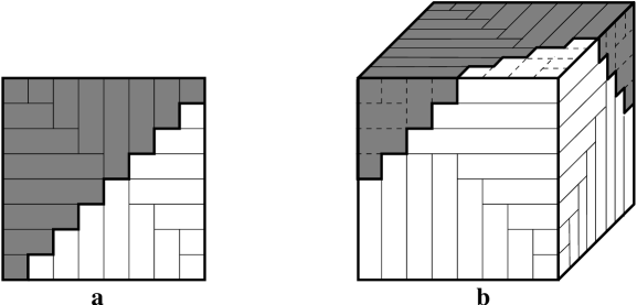
Figure 9: The pattern created by the algorithm in (a) two and (b) three dimensions. The shaded part is filled with the herringbone arrangement for minima sequence, the other half is filled with the arrangement for maxima sequence.

Theorem 2

HERRINGBONE produces an arrangement of a $k$-dimensional cube with dimensions of size $n$ with the spread of

$$\left.\matrix{n^{k}-1-n\left({\left({n+1\over 2}\right)^{k-1}-1}\right),\hfill&\mbox{ if $n$ is odd,}\hfill\cr\cr n^{k}+n-2-\left({n\over 2}\right)^{k-1\over 2}\left({(n+1)\left({n+2\over 2}\right)^{k-1\over 2}-2}\right),\hfill&\mbox{ if $n$ is even, and $k$ is odd,}\hfill\cr\cr n^{k}+n-2-\left({n\over 2}\right)^{k-2\over 2}\left({n+2\over 2}\right)\left({n\left({n+2\over 2}\right)^{k-2\over 2}-1}\right),\hfill&\mbox{ if both $n$ and $k$ are even.}\hfill\cr}\right.$$

Proof.

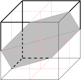
Figure 10: Dividing $3$-dimensional matrix into $8$ pieces. Thick lines show the parts where the border values come from the Herringbone arrangement for the minima sequence.

We shall assume for simplicity that $n$ is odd. For even $n$ the argument works in a similar way. We can divide the matrix into $2^{k}$ pieces by cutting through the middle of each face, including the middle line into both sides that are separated by it. For $k=3$ see Figure 10. The initial and the last pieces, coordinate-wise, are entirely within the minima sequence and the maxima sequence arrangements, respectively. Now each line lies in two of the $2^{k}$ pieces. The central lines go through the initial and the last pieces. The spread in those lines is exactly the maximum difference between the minima and maxima Herringbone arrangements, as calculated above. We will show that the spread in any other line does not exceed that.

There are three types of lines that are not central lines:

1. lines that do not cross the bisecting plane,

2. lines that cross the bisecting plane and the endpoints are neither in the first or the last quadrant of the cube,

3. lines that cross the bisecting plane and one of the endpoints is either in the first or the last quadrant of the cube.

If a line does not cross the bisecting plane, then either its minimum is in the first quadrant or its maximum is in the last quadrant, since only the first and the last quadrants do not have the bisecting plane cutting through them. Without loss of generality, let the line lie completely in the minima arrangement half, and its minimum be in the first quadrant. Then the line’s minimum is at most $\lfloor n/2\rfloor^{k}$ away from the parallel central line’s minimum, while it’s maximum is at least $\lfloor(n/2)^{k}\rfloor-\lfloor n/2\rfloor^{k}$ away from a central maximum. Thus the spread in the line is not greater than the spread in a central line.

The minimum in a line of type (b) is not in the first quadrant, therefore one of the coordinates if the minimum is greater than $\lceil{n/2}\rceil$. As we have mentioned, Herringbone arrangement is a fully monotonic arrangement, the values increasing in the direction of increasing coordinates. Therefore the line’s minimum is greater than the minimum in the parallel central line. Similarly, the line’s maximum is less than the maximum in the parallel central line. Thus the difference between the line’s maximum and minimum, the spread, is less than that in the parallel central line.

We will now consider a line of type (c). Without loss of generality we assume that the line’s minimum is in the first quadrant. Thus the maximum is not in the last quadrant, since all the fixed coordinates of the points on the line are less than $\lceil{n/2}\rceil$. Due to the full monotonicity of the Herringbone arrangement, both the minimum and the maximum in the line are less than those in the parallel central line. We will show that the difference between the central and the line’s minimum is at least the difference between the maxima, thus making the spread in the line at most that in the central line. Moreover, we show that this is true for two lines of type (c) that differ in only one coordinate by $1$, and the spread in the line closer to the central is at least the spread in the other line. Let $a_{t}$ and $a_{t+1}$ be the minima in these lines, and $b_{t}$, $b_{t+1}$ be the maxima, $t<\lfloor n/2\rfloor$. Let $Corner(k,t)$ be the number of cells cut off the corner of size $t$ of a $k$-dimensional cube. Then

$$a_{t+1}-a_{t}\leq(t+1)^{k}-t^{k},$$

and

$$b_{t+1}-b_{t} \geq (n-t)^{k}-Corner\left(k,\left(\left\lfloor{n\over 2}\right\rfloor-(t+1)\right)k\right)-\left((n-(t+1))^{k}-Corner\left(k,\left(\left\lfloor{n\over 2}\right\rfloor-t)\right)k\right)\right)$$

$$= (n-t)^{k}-(n-t-1)^{k}-\left(Corner\left(k,\left(\left\lfloor{n\over 2}\right\rfloor-t-1\right)k\right)-Corner\left(k,\left(\left\lfloor{n\over 2}\right\rfloor-t\right)k\right)\right)$$

Notice that

$$Corner(k,t)=\sum_{i_{1}=1}^{t}{\sum_{i_{2}}^{i_{1}}{\dots\sum_{i_{k-1}}^{i_{k-2}}{i_{k-1}}}}={t+k-1\choose k},$$

Therefore

$$b_{t+1}-b_{t} \geq (n-t)^{k}-(n-t-1)^{k}-\left({\left(\left\lfloor{n\over 2}\right\rfloor-t\right)k-k+k-1\choose k}-{\left(\left\lfloor{n\over 2}\right\rfloor-t\right)k+k-1\choose k}\right)$$

$$= (n-t)^{k}-(n-t-1)^{k}-\left({\left(\left\lfloor{n\over 2}\right\rfloor-t\right)k-1\choose k}-{\left(\left\lfloor{n\over 2}\right\rfloor-t+1\right)k-1\choose k}\right)$$

Thus

$$(b_{t+1}-b_{t})-(a_{t+1}-a_{t}) \geq (n-t)^{k}-(n-t-1)^{k}-\left({\left(\left\lfloor{n\over 2}\right\rfloor-t\right)k-1\choose k}-{\left(\left\lfloor{n\over 2}\right\rfloor-t+1\right)k-1\choose k}\right)-((t+1)^{k}-t^{k})$$

$$= ((n-t)^{k}-(n-t-1)^{k})-((t+1)^{k}-t^{k})-\left({\left(\left\lfloor{n\over 2}\right\rfloor-t\right)k-1\choose k}-{\left(\left\lfloor{n\over 2}\right\rfloor-t+1\right)k-1\choose k}\right)$$

$$t<\left\lfloor{n\over 2}\right\rfloor,\mbox{ therefore }((n-t)^{k}-(n-t-1)^{k})-((t+1)^{k}-t^{k})>0$$

$${\left(\left\lfloor{n\over 2}\right\rfloor-t\right)k-1\choose k}<{\left(\left\lfloor{n\over 2}\right\rfloor-t+1\right)k-1\choose k},\mbox{ therefore }-{\left(\left\lfloor{n\over 2}\right\rfloor-t+1\right)k-1\choose k}>0$$

Thus

$$(b_{t+1}-b_{t})-(a_{t+1}-a_{t})\geq 0$$

and the maximum in a non-central line is further from a central maximum than the minimum in a non-central line from a central minimum. Therefore the spread in a line of type (c) is not greater than the spread in a central line.

We have shown that the maximum spread is achieved in the center and is as calculated above.        

So for a completely filled $k$-dimensional cube the spread is between the lower bound LB and the upper bound UB, where

$$LB=n^{k}-1-\left\lfloor{\left({kn^{k-1}+2\over 2k}\right)^{k\over k-1}}\right\rfloor-\left\lfloor{\left({kn^{k-1}\over 2k}\right)^{k\over k-1}}\right\rfloor$$

and

$$UB=\left.\matrix{n^{k}-1-n\left({\left({n+1\over 2}\right)^{k-1}-1}\right),\hfill&\mbox{ if $n$ is odd,}\hfill\cr\cr n^{k}+n-2-\left({n\over 2}\right)^{k-1\over 2}\left({(n+1)\left({n+2\over 2}\right)^{k-1\over 2}-2}\right),\hfill&\mbox{ if $n$ is even, and $k$ is odd,}\hfill\cr\cr n^{k}+n-2-\left({n\over 2}\right)^{k-2\over 2}\left({n+2\over 2}\right)\left({n\left({n+2\over 2}\right)^{k-2\over 2}-1}\right),\hfill&\mbox{ if both $n$ and $k$ are even.}\hfill\cr}\right.$$

This means that in a multiple descriptions system with all channels of equal capacity the distortion in case of one channel failure is between LB and UB. We address the case of more than one channel failing in Section 2.2.

2.2 Completely Filled Cube: Arbitrary Number of Channels Failing

In the previous section we have obtained the distortion in a multiple descriptions system with equal capacity channels for the case of one channel failing. We now consider the possibility of more than one channel failing. That is, we are concerned with the distortions $D_{k+1}$ through $D_{2^{k}-2}$ in the rate-distortion tuples $(\log n,...,\log n;0,D_{1},...,D_{k},D_{k+1},...,D_{2^{k}-2})$. In the number arrangement domain, we are concerned with designing an arrangement that minimizes the spread in any slice of any dimension.

Notice, however, that the herringbone arrangement maximizes and minimizes the smalls and bigs sequences, respectively, for any slice. Thus we can use the same construction for the algorithm.

The maximum error guaranteed by the algorithm in case of $l$ channel failures is

$$b(\underbrace{\biggl{\lceil}{n-1\over 2}\biggr{\rceil},...,\biggl{\lceil}{n-1\over 2}\biggr{\rceil}}_{\lfloor(k-l)/2\rfloor},\underbrace{\biggl{\lfloor}{n-1\over 2}\biggr{\rfloor},...,\biggl{\lfloor}{n-1\over 2}\biggr{\rfloor}}_{\lceil(k-l)/2\rceil},\underbrace{*,...,*}_{l})-a(\underbrace{\biggl{\lceil}{n-1\over 2}\biggr{\rceil},...,\biggl{\lceil}{n-1\over 2}\biggr{\rceil}}_{\lfloor(k-l)/2\rfloor},\underbrace{\biggl{\lfloor}{n-1\over 2}\biggr{\rfloor},...,\biggl{\lfloor}{n-1\over 2}\biggr{\rfloor}}_{\lceil(k-l)/2\rceil},\underbrace{*,...,*}_{l}),$$

which if $n$ is odd, equals

$$n^{k}-1-\Biggl{(}\biggl{(}{n+1\over 2}\biggr{)}^{k-l}-1\Biggr{)}{(n+1)^{l}+(n-1)^{l}\over 2^{l}},$$

and if $n$ is even, equals

$$n^{k}+n-2-\Biggl{(}\biggl{(}{n\over 2}\biggr{)}^{\bigl{\lceil}{k-l\over 2}\bigr{\rceil}}\biggl{(}{n+2\over 2}\biggr{)}^{l}\biggl{(}\biggl{(}{n+2\over 2}\biggr{)}^{\bigl{\lceil}{k-l\over 2}\bigr{\rceil}}-1\biggr{)}+\biggl{(}{n\over 2}\biggr{)}^{l}\biggl{(}\biggl{(}{n\over 2}\biggr{)}^{\bigl{\lfloor}{k-l\over 2}\bigr{\rfloor}}-1\biggr{)}+$$

$$\biggl{(}{n\over 2}\biggr{)}^{\bigl{\lfloor}{k+l\over 2}\bigr{\rfloor}}\biggl{(}\biggl{(}{n+2\over 2}\biggr{)}^{\bigl{\lfloor}{k-l\over 2}\bigr{\rfloor}}-1\biggr{)}+\biggl{(}{n-2\over 2}\biggr{)}^{l}\biggl{(}\biggl{(}{n\over 2}\biggr{)}^{\bigl{\lceil}{k-l\over 2}\bigr{\rceil}}-1\biggr{)}\Biggr{)}.$$

2.3 The Infinite Diagonal: $n_{i}=\infty,1\leq i\leq k,m=\infty$

We now would like to explore the achievable rate-distortion tuples of the type $(\log n,\log n,...,\log n,0,D_{1},...,D_{2^{k}-2})$ when the original information source is quantized into $m<n^{k}$ integers, where $\log n$ is channel rate. This means that in the corresponding matrix the $m$ numbers do not fill the entire matrix. Vaishampayan [26], [25], [27] designed a solution for this case with two channels which is an arrangement of the numbers into a uniform diagonal. In the next section we examine this solution. However, to avoid the boundary effects, we will first consider the “infinite” diagonal in this section. We consider an arrangement of numbers in a infinite $k$-dimensional diagonal of thickness $l$, that is, any line in the diagonal has exactly $l$ elements in it. This case is also equivalent to deriving the achievable rate-distortion tuples for an unbounded discrete information source and $k$ channels of rate $l$.

Figure 11: Uniform infinite diagonal herringbone arrangements in two and three dimensions.

Again, we will concentrate on the domain of number arrangement. We derive the lower bound on the spread in this case in a similar manner we did in Section 2.1 for the case of a complete cube. We use the herringbone arrangement again to maximize the smalls sequence and to minimize the bigs sequence. Since the smalls and the bigs sequence arrangements can start at any point in the diagonal, we will consider the difference between the sequences relative to the starting points. The lower bound on the spread is the maximum over all lines of the difference between the smallest largest number and the largest smallest nummber. However, in this case this difference turns out to be constant.

Definition 3

A herringbone arrangement of a $k$-dimensional infinite $l$-diagonal is defined inductively as follows. Assign an arbitrary order to the coordinates of the system $\langle i_{1},i_{2},...,i_{k}\rangle$. A herringbone arrangement of $k$-dimensional $0$-diagonal is empty. A herringbone arrangement of a $0$-dimensional diagonal is any arrangement of one number in a cell.

Given a herringbone arrangement of the $k$-dimensional diagonal up to coordinate $t_{i}$ in dimension $i$, we define a larger herringbone arrangement inductively:

• project the existing arrangement onto the $(k-1)$-dimensional hyperplanes $(*,...,*,t_{i},*,...,*)$, limited to the diagonal,

• calculate the volume of each projection,

• recursively fill the largest volume projection (using coordinate order to break ties) with the herringbone arrangement for $k-1$ dimensions.

We denote the element in the cell $(i_{1},...,i_{k})$ of the $k$-dimensional herringbone arrangement by $HB_{k}(i_{1},...,i_{k})$. Examples of a herringbone arrangement of a diagonal are shown in Figure 11.

Lemma 3

The herringbone arrangement of values in a $k$-dimensional diagonal maximizes the smalls sequence – the ascending list of the smallest numbers in a line – for that matrix.

The proof is similar to the proof of Lemma 2.

Corollary 1

If the smallest number in line $(i_{1},...,*,...,i_{k})$ of the herringbone arrangement is $a_{j}$, then the smallest number in line $(i_{1}+1,...,*,...,i_{k}+1)$ is

$$a_{j}+\sum_{i=0}^{k-1}{\lfloor l/2\rfloor^{i}\lceil l/2\rceil^{k-1-i}}=\left\{\matrix{a_{j}+k(l/2)^{k-1},\hfill&\mbox{ if $l$ is even,}\cr\cr a_{j}+{(l-1)^{k}+(l+1)^{k}\over 2^{k}},\hfill&\mbox{ if $l$ is odd.}\cr}\right.$$

Similarly,

Corollary 2

If the largest number in line $(i_{1},...,*,...,i_{k})$ of the herringbone arrangement is $b_{j}$, then the largest number in line $(i_{1}+1,...,*,...,i_{k}+1)$ is

$$b_{j}+\sum_{i=0}^{k-1}{\lfloor l/2\rfloor^{i}\lceil l/2\rceil^{k-1-i}}=\left\{\matrix{b_{j}+k(l/2)^{k-1},\hfill&\mbox{ if $l$ is even,}\cr\cr b_{j}+{(l-1)^{k}+(l+1)^{k}\over 2^{k}},\hfill&\mbox{ if $l$ is odd.}\cr}\right.$$

Thus, combining the results of Corollary 1 and Corollary 2, the difference $b_{j}-a_{j}$ remains constant along any diagonal. That is, the difference between the largest and the smallest numbers in line $(i_{1},i_{2},...,*,...,i_{k})$ equals that of line $(i_{1}+s,i_{2}+s,...,*,...,i_{k}+s)$ for some integer $s$. To see this, notice that while we start the smalls arrangement from $0$ at some point, since the diagonal is infinite, we can continue the arrangement in the other direction using increasingly smaller numbers. Similarly with the bigs arrangement, we can continue it in the direction of the increasing of coordinates using larger numbers. Thus the smalls and the bigs arrangements are the same arrangements, offset by a certain value. This arrangements are also “facing” opposite directions: the herringbone arrangement can be viewed as cones stacked into each other, and in case of the smalls sequence the “cones” face the direction of the coordinate decrease, while in the bigs sequence “cones” face the coordinate increase direction. However, the brims of these cones from both sequences coincide, and since that is where the smallest and the largest numbers in each line occur, the difference along any diagonal remains constant.

A consequence of the structure of the herringbone arrangement is the fact that the difference is maximized over the central diagonal. That is, if $(t,t,...,t)$ is a cell in the center of the diagonal, then the maximum difference is achieved for any line $(t+s,t+s,...,*,...,t+s)$, where $s$ is some integer, and equals to the difference

$$HB(t+\lfloor l/2\rfloor,t,...,t)-HB(t-\lceil l/2\rceil,t,...,t)=$$

$$(\lceil l/2\rceil-1)\sum_{i=0}^{k-1}{\lfloor l/2\rfloor^{i}\lceil l/2\rceil^{k-1-i}}+\lceil l/2\rceil^{k-1}.$$

2.4 The Incomplete Cube: $n_{i}=n,1\leq i\leq k;m\leq n^{k}<\infty$

Suppose we have an arbitrary quantity of $m\leq n^{k}$ numbers to be arranged in a $n\times\cdots\times n$ $k$-dimensional cube. This corresponds to the information source being quantized into $m$ integers, where $\log m$ is less than the combined channel rates. At first glance, the diagonal arrangement gives the least distortion. That is precisely the shape used by Vaishampayan in [26], [25], [27]. We show, however, that diagonal arrangement is not the best possible and a lower distortion is possible for these rates.

Consider a diagonal arrangement limited to the $n^{k}$ cube. It is a restriction of an infinite diagonal, thus the bound on the spread is the same over the true diagonal part of the arrangement, away from the boundary effect. However, the boundary parts of the arrangement are complete cubes of size $\lfloor l/2\rfloor^{k}$, and the spread there is the spread in a complete cube derived in Section 2.1. By comparing the two spreads, in the boundary cubic parts and in the diagonal part, we can show that the spread on the diagonal is always greater. Thus the spread is dominated by the diagonal part, as long there is a true diagonal part. That is, if $l\leq n$, then there is at least one complete line in each dimension which belongs entirely to the diagonal, and the spread in this line dominates the overall spread in the matrix. But this means that we can increase the size of the initial cubic part, decrease the width of the diagonal part, thus decreasing the overall spread. Not only that, but we can decrease the spread even more by introducing non-overlapping cubic parts along the diagonal, thus, by balancing the entire structure, making all of the cubic part smaller. This construction i sdemonstrated in Figure 12. The spread in this arrangement is better than the diagonal. However currently we do not have a proof whether this arrangement is optimal or not.

Figure 12: Possibly an optimal arrangement for for an incompletely filled cube.

Now, if $l>n$, then the initial cubic parts of the diagonal overlap. Remembering from Section 2.1, the maximum spread of the entirely filled cube is the spread in line $(\lceil(n-1)/2\rceil,...,*,...,\lfloor(n-1)/2\rfloor)$, which is a line in the intersection of the first-quadrant cube and the last-quadrant cube. Those are precisely the cubic parts of the diagonally filled cube. Since the spread of a cube optimally filled with $m<n^{k}$ numbers is at most the spread of the cube filled with $n^{k}$ numbers, in the case of the overlapping cubic parts of the diagonal the spread is the the same as in a completely filled cube. However, once again, this proves only the upper bound on the optimal arrangement, not the lower bound.

2.5 Unequal Channel Rates

There are currently no known existing results for the case of unequal channel rates, that is, unequal $n_{i}$’s. Our approach would provide the first non-trivial lower and upper bounds. Before the final calculations can be made, however, we need to generalize the concept of the integer bisecting hyperplane to non-cubic matrices. In 1965 Bresenham [5] gave an algorithm that approximates real lines on a discrete grid. Since our algorithm for the matrix arrangement uses two Herringbone arrangements put together at a bisecting hyperplane, we need to find an appropriate generalization of Bresenham’s algorithm to describe that hyperplane for a matrix with unequal dimension sizes.

3 Conclusions

We have studied the problem of multiple description scalar quantizers. We have considered the question of describing the achievable rate-distortion tuples. The problem has been formulated as a combinatorial optimization problem of arranging numbers in a matrix. It has been noted that this formulation is equivalent to a graph theory problem of finding minimal bandwidth of cartesian products of cliques.

We have proposed a technique for deriving lower bounds on the distortion at given channel rates. The approach is constructive thus allowing an algorithm that gives a fairly tight upper bound. For the case of two communication channels with equal rates the bounds coincide thus giving the precise lowest achievable distortion at fixed rates. To the best of our knowledge, this is the first result concerning the system with more than two communication channels.

4 Acknowledgments

We would like to thank Sergio Servetto for bringing this problem to our attention, Douglas West for pointing out the relevance to the graph bandwidth problem and helpful suggestions, Ari Trachtenberg, Mitch Harris, Jeff Erickson, and Ralf Koetter for many fruitful discussions.

References

- [1] Ahlswede, R., “The rate-distortion region for multiple descriptions without excess rate”, IEEE Transactions on Information Theory, 31 (1985), 721–726.
- [2] Batllo, J- C. and V.A. Vaishampayan, “Multiple description transform codes with an application to packetized speech”, IEEE International Symposium on Information Theory - Proceedings, 1994, IEEE, Piscataway, NJ, USA.
- [3] Berger, T. and Z. Zhang, “Minimum breakdown degradation in binary source encoding”, IEEE Transactions on Information Theory, 29 (1983), 807–814.
- [4] Bezrukov, S. L., “Edge Isoperimetric Problems on Graphs”, Graph Theory and Combinatorial Biology, Balatonlelle 1996, Budapest 1999, 157–197.
- [5] Bresenham, J., “Algorithm for computer control of digital plotter”, IBM Systems Journal 4 (1965), 25–30.
- [6] Buzi, L., V.A. Vaishampayan and R. Laroia, “Design and asymptotic performance of a structured multiple description vector quantizer”, IEEE International Symposium on Information Theory - Proceedings, 1994, IEEE, Piscataway, NJ, USA.
- [7] Chinn, P. Z., J. Chvátalová, A.K. Dewdney, and N.E. Gibbs, “The Bandwidth Problem for Graphs and Matrices – A Survey”, Journal of Graph Theory, 6 (1982), 223–254.
- [8] El Gamal, A. A. and T.M. Cover, “Achievable rates for multiple descriptions”, IEEE Transactions on Information Theory, 28 (1982), 851–857.
- [9] Feige, U., “Approximating the bandwidth via volume respecting embedding”, 13th Annual ACM Symposium on Theory of Computing-Proceedings, 1998, ACM, Dallas, TX, USA.
- [10] Fishburn, P, P. Tetali, and P. Winkler, “Optimal linear arranagment of a rectangular grid”, Preprint, 1999.
- [11] Gale, D. and R. Karp, “A phenomenon in the Theory of Sorting”, Journal of Computer and System Sciences 6, 103-115 (1972)
- [12] Graham, R. L., D.E. Knuth and O. Patashnik, Concrete Mathematics: A Foundation For Computer Science, 2nd ed., Addison-Wesley, 1994.
- [13] Harper, L. H, “Optimal assignments of numbers to vertices”, Journal of SIAM, 12, Vol.1, (March 1964), 131–135.
- [14] Harper, L. H, “Optimal Numberings and Isoperimetric Problems on Graphs”, Journal of Combinatorial Theory, 1 (1966), 385–393.
- [15] Harper, L. H, “On an isoperimetric problem for Hamming graphs”, Discrete Applied Mathematics, 95 (1999), 258–309.
- [16] Henrich, U. and M. Stiebitz, “On the Bandwidth of graph products”, Journal of information processing and cybernetics, 28 (1992) 113–125.
- [17] Jayant, N. S., “Subsampling of a DPCM speech channel to provide two self-contained half-rate channels”, The Bell System Technical Journal, 60 (1981), 501–501.
- [18] Jayant, N. S. and S.W. Christensen, “Effect of packet losses in waveform coded speech and improvements due to odd-even sample interpolation procedure”, IEEE Transactions on Communications, 29 (1981), 101–109.
- [19] Karpinski, M., J. Wirtgen and A. Zelikovsky, “An approximation algorithm for the bandwidth problem on dense graphs”, ECCC TR97-017.
- [20] Kloks, T., D. Kratsch and H. Muller, “Approximating the bandwidth for asteroidal triple-free graphs”, Algorithms-ESA ’95, Paul Spirakis (Ed.), Lecture Notes in computer Science 979, 434–447.
- [21] Lawler, E. L., Combinatorial optimization : networks and matroids, New York : Holt, Rinehart and Winston, 1976.
- [22] Nakano, K., “Linear layout of generalized hypercubes”, Proceedings of WG’93, Lecture Notes in Computer Science 790, Springer Verlag, 1994, 364–375.
- [23] Ozarow, L., “On a source coding problem with two channels and three receivers”, The Bell System Technical Journal, 59 (1980), 1909–1921.
- [24] Shannon, C. E., “Coding theorems for discrete source with fidelity criterion”, IRE National Convention Record, 4 (1959), 142–163.
- [25] Vaishampayan, V. A., “Vector quantizer design for diversity systems”, in Proceedings of 25 Annual Conference on Inform. Sci. Syst., Johns Hopkins University, Mar. 20–22, 1991, 564–569.
- [26] Vaishampayan, V. A.,“Design of multiple description scalar quantizers,” IEEE Transactions on Information Theory, 93 (1993), 821–834.
- [27] Vaishampayan, V. A. and J. Domaszewicz, “Design of entropy-constrained multiple-description scalar quantizers”, IEEE Transactions on Information Theory, 40 (1994), 245–250.
- [28] West, D. B., Introduction to Graph Theory, Prentice Hall, 1996.
- [29] West, D. B., personal communication.
- [30] Witsenhausen, H. S. and A.D. Wyner, “Source coding for multiple descriptions II: A binary source”, The Bell System Technical Journal, 60 (1981), 2281–2292.
- [31] Wolf, J. K., A.D. Wyner and J. Ziv, “Source coding for multiple descriptions”, The Bell System Technical Journal, 59 (1980), 1417–1426.
- [32] Yang, S.- M. and V.A. Vaishampayan, “Low-delay communication for Rayleigh fading channels: an application of the multiple description quantizer”, IEEE Transactions on Communications, 43 (1995), 2771–2783.
- [33] Zhang, Z. and T. Berger, “New results in binary multiple description”, IEEE Transactions on Information Theory, 33 (1987), 502–521.