Provably Fast and Accurate Recovery of Evolutionary Trees through Harmonic Greedy Triplets

Abstract

We give a greedy learning algorithm for reconstructing an evolutionary tree based on a certain harmonic average on triplets of terminal taxa. After the pairwise distances between terminal taxa are estimated from sequence data, the algorithm runs in ${\cal O}(n^{2})$ time using ${\cal O}(n)$ work space, where $n$ is the number of terminal taxa. These time and space complexities are optimal in the sense that the size of an input distance matrix is $n^{2}$ and the size of an output tree is $n$. Moreover, in the Jukes-Cantor model of evolution, the algorithm recovers the correct tree topology with high probability using sample sequences of length polynomial in (1) $n$, (2) the logarithm of the error probability, and (3) the inverses of two small parameters.

1 Introduction

Algorithms for reconstructing evolutionary trees are useful tools in biology [16, 22]. These algorithms usually compare aligned character sequences for the terminal taxa in question to infer their evolutionary relationships. In the past, such characters were often categorical variables of morphological features; newer studies have taken advantage of available biomolecular sequences. This paper focuses on datasets of the latter type.

We present a new learning algorithm, called Fast Harmonic Greedy Triplets (Fast-HGT), using a greedy strategy based on a certain harmonic average on triplets of terminal taxa. After the pairwise distances between terminal taxa are estimated from their observed sequences, Fast-HGT runs in ${\cal O}(n^{2})$ time using ${\cal O}(n)$ work space, where $n$ is the number of terminal taxa. These time and space complexities are optimal in the sense that $n^{2}$ is the size of an input distance matrix and $n$ is the size of an output tree. An earlier variant of Fast-HGT takes ${\cal O}(n^{5})$ time [5]. In the Jukes-Cantor model of sequence evolution generalized for an arbitrary alphabet [22], Fast-HGT is proven to recover the correct topology with high probability while requiring sample sequences of length $\ell$ polynomial in (1) $n$, (2) the logarithm of the error probability, and (3) the inverses of two small parameters (Theorem 17). In subsequent work [6], Fast-HGT and its variants are shown to have similar theoretical performance in more general Markov models of evolution.

Among the related work, there are four other algorithms which have essentially the same guarantee on the length $\ell$ of sample sequences. These are the Dyadic Closure Method (DCM) [10] and the Witness-Antiwitness Method (WAM) [11] of Erdős, Steel, Székely, and Warnow, the algorithm of Cryan, Goldberg, and Goldberg (CGG) [4], and the DCM-Buneman algorithm of Huson, Nettles, and Warnow [18]. Not all of these results analyzed the space complexity. In terms of time complexity, DCM-Buneman is not a polynomial-time algorithm. CGG runs in polynomial time, whose degree has not been explicitly determined but which appears to be higher than $n^{2}$. DCM takes ${\cal O}(n^{5}\log n)$ time to assemble ${\cal O}(n^{4})$ quartets using ${\cal O}(n^{4})$ space. The two versions of WAM take ${\cal O}(n^{6}\log n)$ and ${\cal O}(n^{4}\log n\log\ell)$ time, respectively. In the uniform and Yule-Harding models of randomly generating trees, with high probability, these two latter running times are reduced to ${\cal O}(n^{3}\mathop{\rm polylog}\nolimits n)$ and ${\cal O}(n^{2}\mathop{\rm polylog}\nolimits n)$, respectively. Under these two tree distributions, Erdős et al. [10] further showed that with high probability, the required sample size of DCM is polylogarithmic in $n$; this bound also applies to WAM, CGG, DCM-Buneman, and Fast-HGT.

Among the algorithms with no known comparbale guarantees on $\ell$, the Neighbor Joining Method of Saitou and Nei [22] runs in ${\cal O}(n^{3})$ time and reconstructs many trees highly accurately in practice, although the best known upper bound on its required sample size is exponential in $n$ [3]. Maximum likelihood methods [15, 14] are not known to achieve the optimal required sample size as such methods are usually expected to [20]; moreover, all their known implementations take exponential time to find local optima, and none can find provably global optima. Parsimony methods aim to compute a tree that minimizes the number of mutations leading to the observed sequences [13]; in general, such optimization is NP-hard [8]. Some algorithms strive to find an evolutionary tree among all possible trees to fit the observed distances the best according to some metric [1]; such optimization is NP-hard for $L_{1}$ and $L_{2}$ norms [7] and for $L_{\infty}$ [1].

A common goal of the above algorithms is to construct a tree with the same topology as that of the true tree. In contrast, the work on PAC-learning the true tree in the $j$-State General Markov Model [21] aim to construct a tree which is close to the true tree in terms of the leaf distribution in the sense of Kearns et al. [19] but which need not be the same as the true tree. Farach and Kannan [12] gave an ${\cal O}(n^{2}\ell)$-time algorithm (FK) for the symmetric case of the $2$-state model provided that all pairs of leaves have a sufficiently high probability of being the same. Ambainis, Desper, Farach, and Kannan [2] gave a nearly tight lower bound on $\ell$ for achieving a given variational distance between the true tree and the reconstructed tree. As for obtaining the true tree, the best known upper bound on $\ell$ required by FK is exponential in $n$. CGG [4] also improves upon FK to PAC-learn in the general $2$-state model without the symmetry and leaf similarity constraints.

The remainder of the paper is organized as follows. Section 2 reviews the generalized Jukes-Cantor model of sequence evolution and discusses distance-based probabilistic techniques. Section 3 gives Fast-HGT. Section 4 concludes the paper with some directions for further research.

2 Model and techniques

Section 2.1 defines the model of evolution used in the paper. Section 2.2 defines our problem of recovering evolutionary trees from biological sequences. Sections 2.3 through 2.5 develop basic techniques for the problem.

2.1 A model of sequence evolution

This paper employs the generalized Jukes-Cantor model [22] of sequence evolution defined as follows. Let $m\geq 2$ and $n\geq 3$ be two integers. Let ${\cal A}=\left\{a_{1},\ldots,a_{m}\right\}$ be a finite alphabet. An evolutionary tree $T$ for ${\cal A}$ is a rooted binary tree of $n$ leaves with an edge mutation probability $p_{e}$ for each tree edge $e$. The edge mutation probabilities are bounded away from $0$ and $1-\frac{1}{m}$, i.e., there exist $f$ and $g$ such that for every edge $e$ of $T$, $0<f\leq p_{e}\leq g<1-\frac{1}{m}.$ Given a sequence $s_{1}\cdots s_{\ell}\in{\cal A}^{\ell}$ associated with the root of $T$, a set of $n$ mutated sequences in ${\cal A}^{\ell}$ is generated by $\ell$ random labelings of the tree at the nodes. These $\ell$ labelings are mutually independent. The labelings at the $j$-th leaf give the $j$-th mutated sequence $s_{1}^{(j)}\cdots s_{\ell}^{(j)}$, where the $i$-th labeling of the tree gives the $i$-th symbols $s_{i}^{(1)},\ldots,s_{i}^{(n)}$. The $i$-th labeling is carried out from the root towards the leaves along the edges. The root is labeled by $s_{i}$. On edge $e$, the child’s label is the same as the parent’s with probability $1-p_{e}$ or is different with probability $\frac{p_{e}}{m-1}$ for each different symbol. Such mutations of symbols along the edges are mutually independent.

2.2 Problem formulation

The topology $\Psi(T)$ of $T$ is the unrooted tree obtained from $T$ by omitting the edge mutation probability and by replacing the two edges $e_{1}$ and $e_{2}$ between the root and its children with a single edge $e_{0}$. Note that the leaves of $\Psi(T)$ are labeled with the same sequences as in $T$, but $\Psi(T)$ need not be labeled otherwise. The weighted topology $\Psi_{\rm w}(T)$ of $T$ is $\Psi(T)$ where each edge $e\neq e_{0}$ of $\Psi(T)$ is further weighted by its edge mutation probability $p_{e}$ in $T$ and for technical reasons, the edge $e_{0}$ is weighted by $1-(1-p_{e_{1}})(1-p_{e_{2}})$.

For technical convenience, the weight of each edge $XY$ in $\Psi_{\rm w}(T)$ is often replaced by a certain edge length, such as $\Delta_{XY}$ in Equation (5), from which the weight of $XY$ can be efficiently determined.

The weighted evolutionary topology problem is that of taking $n$ mutated sequences as input and recovering $\Psi_{\rm w}(T)$ with high accuracy and high probability. Fast-HGT is a learning algorithm for this problem.

Remark. The special treatment for $e_{1}$ and $e_{2}$ is due to the fact that the root sequence may be entirely arbitrary and thus, in general, no algorithm can place the root accurately. This is consistent with the fact that the root sequence is not directly observable in practice, and locating the root requires considerations beyond those of general modeling [22]. If the root sequence is also given as input, Fast-HGT can be modified to locate the root and the weights of $e_{1}$ and $e_{2}$ in a straightforward manner.

2.3 Probabilistic closeness

Fast-HGT is based on a notion of probabilistic closeness between nodes. For the $i$-th random labeling of $T$, we identify each node of $T$ with the random variable $X_{i}$ that gives the labeling at the node. Note that since $s_{1}\cdots s_{\ell}$ may be arbitrary, the random variables $X_{i}$ for different $i$ are not necessarily identically distributed. For brevity, we often omit the index $i$ of $X_{i}$ in a statement if the statement is independent of $i$.

For nodes $X$ and $Y\in T$, let $p_{XY}={\rm Pr}\!\left\{\,{X\neq Y}\,\right\}.$ The closeness of $X$ and $Y$ is

$$\sigma_{XY}={\rm Pr}\!\left\{\,{X=Y}\,\right\}-\frac{1}{m-1}{\rm Pr}\!\left\{\,{X\neq Y}\,\right\}=1-\alpha p_{XY},\mbox{where}\ \alpha=\frac{m}{m-1}.$$ (1)

Lemma 1 (folklore).

If node $Y$ is on the path between two nodes $X$ and $Z$ in $T$, then $\sigma_{XZ}=\sigma_{XY}\sigma_{YZ}$.

If $X$ and $Y$ are leaves, their closeness is estimated from sample sequences as

$$\hat{\sigma}_{XY}=\frac{1}{\ell}\sum_{i=1}^{\ell}I_{\hat{X}_{i}\hat{Y}_{i}},$$ (2)

where $\hat{X}_{1},\ldots,\hat{X}_{\ell}$ and $\hat{Y}_{1},\ldots,\hat{Y}_{\ell}$ are the symbols at positions $1,\ldots,\ell$ of the observed sample sequences for the two leaves, and

$$I_{xy}=\left\{\begin{array}[]{ll}\frac{-1}{m-1}&\mbox{ if }x\neq y;\\ 1&\mbox{ if }x=y.\end{array}\right.$$

The next lemma is useful for analyzing the estimation given by Equation (2).

Lemma 2.

For $\epsilon>0$,

$${\rm Pr}\!\left\{\,{\frac{\hat{\sigma}_{XY}}{\sigma_{XY}}\leq 1-\epsilon}\,\right\} \leq \exp\left(-\frac{2}{\alpha^{2}}\ell\sigma_{XY}^{2}\epsilon^{2}\right);$$ (3)

$${\rm Pr}\!\left\{\,{\frac{\hat{\sigma}_{XY}}{\sigma_{XY}}\geq 1+\epsilon}\,\right\} \leq \exp\left(-\frac{2}{\alpha^{2}}\ell\sigma_{XY}^{2}\epsilon^{2}\right).$$ (4)

Proof.

By Equation (2),

$${\rm Pr}\!\left\{\,{\frac{\hat{\sigma}_{XY}}{\sigma_{XY}}\leq 1-\epsilon}\,\right\} = {\rm Pr}\!\left\{\,{\sum_{i=1}^{\ell}\left(I_{X_{i}Y_{i}}-\sigma_{XY}\right)\leq-\ell\sigma_{XY}\epsilon}\,\right\};$$

$${\rm Pr}\!\left\{\,{\frac{\hat{\sigma}_{XY}}{\sigma_{XY}}\geq 1+\epsilon}\,\right\} = {\rm Pr}\!\left\{\,{\sum_{i=1}^{\ell}\left(I_{X_{i}Y_{i}}-\sigma_{XY}\right)\geq\ell\sigma_{XY}\epsilon}\,\right\}.$$

Since $\frac{-1}{m-1}\leq I_{X_{i}Y_{i}}\leq 1$ and $\mbox{\rm{I}\kern-1.66702pt{E}}\!\left[\,{I_{X_{i}Y_{i}}-\sigma_{XY}}\,\right]=0$, we use Hoeffding’s inequality [17] on sums of independent bounded random variables to have Equations (3) and (4). ∎

2.4 Distance and harmonic mean

The distance of nodes $X$ and $Y\in T$ is

$$\Delta_{XY}=-\ln\sigma_{XY}.$$ (5)

For an edge $XY$ in $T$, $\Delta_{XY}$ is called the edge length of $XY$.

Fast-HGT uses Statement 3 of the next corollary to locate internal nodes of $T$.

Corollary 3.

Let $X$, $Y$, and $Z$ be nodes in $T$.

1. If $X\neq Y$, then $\Delta_{XY}=\Delta_{YX}>0$. Also, $\Delta_{XX}=0$.

2. If $Y$ is on the path between $X$ and $Z$ in $T$, then $\Delta_{XZ}=\Delta_{XY}+\Delta_{YZ}$.

3. For any $\sigma$ with $\sigma_{XY}\leq\sigma<1$, there is a node $P$ on the path between $X$ and $Y$ in $T$ such that $\sigma(1-\alpha g)^{1/2}\leq\sigma_{XP}\leq\sigma(1-\alpha g)^{-1/2}.$ Furthermore, if $\sigma_{XY}(1-\alpha g)^{1/2}<\sigma<(1-\alpha g)^{-1/2},$ then $P$ is distinct from $X$ and $Y$.

Proof.

Statements 1 and 2 follow from Equation (1) and Lemma 1. Statement 3 becomes straightfoward when restated in terms of distance as follows. For any $\Delta$ with $\Delta_{XY}\geq\Delta>0$, there is a node $P$ on the path between $X$ and $Y$ in $T$ such that $\Delta+\frac{-\ln(1-\alpha g)}{2}\geq\Delta_{XP}\geq\Delta-\frac{-\ln(1-\alpha g)}{2}.$ Furthermore, if $\Delta_{XY}-\frac{-\ln(1-\alpha g)}{2}>\Delta>\frac{-\ln(1-\alpha g)}{2},$ then $P$ is distinct from $X$ and $Y$. ∎

If $X$ and $Y$ are leaves, their distance is estimated from sample sequences as

$$\hat{\Delta}_{XY}=\left\{\begin{array}[]{ll}-\ln\hat{\sigma}_{XY}&\mbox{ if }\hat{\sigma}_{XY}>0;\\ \infty&\mbox{ otherwise.}\end{array}\right.$$ (6)

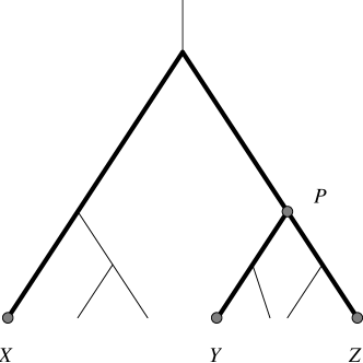
Fig. 1: $P$ is the center of triplet $XYZ$.

A triplet $XYZ$ consists of three distinct leaves $X$, $Y$, and $Z$ of $T$. There is an internal node $P$ in $T$ at which the pairwise paths between the leaves in $XYZ$ intersect; see Figure 1. $P$ is the center of $XYZ$, and $XYZ$ defines $P$. Note that a star is formed by the edges on the paths between $P$ and the three leaves in $XYZ$.

By Corollary 3(2), the distance between $P$ and a leaf in $XYZ$, say, $X$, can be obtained as $\Delta_{XP}=\frac{\Delta_{XY}+\Delta_{XZ}-\Delta_{YZ}}{2},$ which is estimated by

$$\hat{\Delta}_{XP}=\frac{\hat{\Delta}_{XY}+\hat{\Delta}_{XZ}-\hat{\Delta}_{YZ}}{2}.$$ (7)

The closeness of $XYZ$ is $\sigma_{XYZ}=\frac{3}{\frac{1}{\sigma_{XY}}+\frac{1}{\sigma_{XZ}}+\frac{1}{\sigma_{YZ}}},$ which is estimated by $\hat{\sigma}_{XYZ}=\frac{3}{\frac{1}{\hat{\sigma}_{XY}}+\frac{1}{\hat{\sigma}_{XZ}}+\frac{1}{\hat{\sigma}_{YZ}}}.$ $XYZ$ is called positive if $\hat{\sigma}_{XY}$, $\hat{\sigma}_{XZ}$, and $\hat{\sigma}_{YZ}$ are all positive.

The next corollary relates $\sigma_{XYZ}$ and the pairwise closenesses of $X$, $Y$, and $Z$.

Corollary 4.

If $\sigma_{XP}\leq\sigma_{YP}\leq\sigma_{ZP}$, then $\sigma_{XY}\leq\sigma_{XZ}\leq\sigma_{YZ}$, $\sigma_{XZ}\geq\frac{2}{3}\sigma_{XYZ}$, and $\sigma_{YP}^{2}\geq\frac{1}{3}\sigma_{XYZ}$.

Proof.

This corollary follows from Lemma 1 and simple algebra. ∎

The next lemma relates $\sigma_{XYZ}$ to the probability of overestimating the distance between $P$ and a leaf in $XYZ$ using Equation (7).

Lemma 5.

For $0<\epsilon<1$,

$${\rm Pr}\!\left\{\,{\hat{\Delta}_{XP}-\Delta_{XP}\geq\frac{-\ln(1-\epsilon)}{2}}\,\right\}\leq 3\exp\left(-\frac{2}{9\alpha^{2}}\ell\sigma_{XYZ}^{2}\epsilon^{2}\right).$$

Proof.

See §A.1. ∎

2.5 Basis of a greedy strategy

Let $d_{XY}$ denote the number of edges in the path between two leaves $X$ and $Y$ in $T$. By Lemma 1, $\sigma_{XY}$ can be as small as $(1-\alpha g)^{d_{XY}}$. Thus, the larger $d_{XY}$ is, the more difficult it is to estimate $\sigma_{XY}$ and $\Delta_{XY}$. This intuition leads to a natural greedy strategy outlined below that favors leaf pairs with small $d_{XY}$ and large $\sigma_{XY}$.

The g-depth of a node in a rooted tree $T^{\prime}$ is the smallest number of edges in a path from the node to a leaf. Let $e$ be an edge between nodes $u_{1}$ and $u_{2}$. Let $T^{\prime}_{1}$ and $T^{\prime}_{2}$ be the subtrees of $T^{\prime}$ obtained by cutting $e$ which contain $u_{1}$ and $u_{2}$, respectively. The g-depth of $e$ in $T^{\prime}$ is the larger of the g-depth of $u_{1}$ in $T^{\prime}_{1}$ and that of $u_{2}$ in $T^{\prime}_{2}$. The g-depth of a rooted tree is the largest possible g-depth of an edge in the tree. (The prefix g emphasizes that this usage of depth is nonstandard in graph theory.)

Let $d$ be the $g$-depth of $T$. Variants of the next lemma have proven very useful and insightful; see, e.g., [9, 11, 10].

Lemma 6.

1. $d\leq 1+\lfloor{\log_{2}(n-1)}\rfloor.$

2. Every internal node $P$ of $T$ except the root has a defining triplet $XYZ$ such that $d_{XP},d_{YP}$, and $d_{ZP}$ are all at most $d+1$ and thus, $\sigma_{XYZ}\geq(1-\alpha g)^{2(d+1)}$. Every leaf of $T$ is in such a triplet.

Proof.

The proof is straightforward. Note that the more unbalanced $T$ is, the smaller its g-depth is. ∎

In $T$, the star formed by a defining triplet of an internal node contains the three edges incident to the internal node. Thus, $\Psi(T)$ can be reconstructed from triplets described in Lemma 6(2) or those with similarly large closenesses. This observation motivates the following definitions. Let

$$\sigma_{\mathrm{lg}}=\frac{3\sqrt{2}}{2}\left(\frac{\sqrt{2}-1}{\sqrt{2}+1}\right)^{2}(1-\alpha g)^{2d+4};\ \ \sigma_{\mathrm{sm}}=\frac{\sigma_{\mathrm{lg}}}{\sqrt{2}};\ \ \sigma_{\mathrm{md}}=\frac{\sigma_{\mathrm{lg}}+\sigma_{\mathrm{sm}}}{2}.$$

Remark. The choice of $\sigma_{\mathrm{lg}}$ is obtained by solving Equations (3.3), (3.3) and (3.3).

A triplet $XYZ$ is large if $\sigma_{XYZ}\geq\sigma_{\mathrm{lg}}$; it is small if $\sigma_{XYZ}\leq\sigma_{\mathrm{sm}}$. Note that by Lemma 6(2), each nonroot internal node of $T$ has at least one large defining triplet.

Lemma 7.

The first inequality below holds for all large triplets $XYZ$, and the second for all small triplets.

$${\rm Pr}\!\left\{\,{\hat{\sigma}_{XYZ}\leq\sigma_{\mathrm{md}}}\,\right\} \leq \exp\left(-\frac{\left(\sqrt{2}-1\right)^{2}}{36\alpha^{2}}\ell\sigma_{\mathrm{lg}}^{2}\right);$$ (8)

$${\rm Pr}\!\left\{\,{\hat{\sigma}_{XYZ}\geq\sigma_{\mathrm{md}}}\,\right\} \leq \exp\left(-\frac{\left(\sqrt{2}-1\right)^{2}}{36\alpha^{2}}\ell\sigma_{\mathrm{lg}}^{2}\right).$$ (9)

Proof.

See §A.2. ∎

A nonroot internal node of $T$ may have more than one large defining triplet. Consequently, since distance estimates contain errors, we may obtain an erroneous estimate of $\Psi(T)$ by reconstructing the same internal node more than once from its different large defining triplets. To address this issue, Fast-HGT adopts a threshold $0<\Delta_{\min}<\frac{-\ln(1-\alpha f)}{2}$ based on the fact that the distance between two distinct nodes is at least $-\ln(1-\alpha f)$; also let $c=\frac{\Delta_{\min}}{-\ln(1-\alpha f)}.$ Fast-HGT considers the center $P$ of a triplet $XYZ$ and the center $Q$ of another triplet $XUV$ to be separate if and only if

$$|\hat{\Delta}_{XP}-\hat{\Delta}_{XQ}|\geq\Delta_{\min},\$$ (10)

where $\hat{\Delta}_{XP}=(\hat{\Delta}_{XY}+\hat{\Delta}_{XZ}-\hat{\Delta}_{YZ})/2\ \mbox{and}\ \hat{\Delta}_{XQ}=(\hat{\Delta}_{XU}+\hat{\Delta}_{XV}-\hat{\Delta}_{XV})/2.$ Notice that two triplet centers can be compared in this manner only if the triplets share at least one leaf. The next lemma shows that a large triplet’s center is estimated within a small error with high probability.

Lemma 8.

Let $P$ be the center of a triplet $XYZ$. If $XYZ$ is not small, then

$${\rm Pr}\!\left\{\,{\left|\hat{\Delta}_{XP}-\Delta_{XP}\right|\geq\frac{\Delta_{\min}}{2}}\,\right\} \leq 7\exp\left(-\frac{c^{2}}{81}\ell\sigma_{\mathrm{lg}}^{2}f^{2}\right).$$ (11)

Proof.

See §A.3. ∎

We next define and analyze two key events ${\cal E}_{\rm c}$ and ${\cal E}_{\rm g}$ as follows. The subscripts c and g denote the words greedy and center, respectively.

• ${\cal E}_{\rm c}$ is the event that for every triplet $XYZ$ that is not small, $\left|\hat{\Delta}_{XP}-\Delta_{XP}\right|<\frac{\Delta_{\min}}{2}$, $\left|\hat{\Delta}_{YP}-\Delta_{YP}\right|<\frac{\Delta_{\min}}{2}$, and $\left|\hat{\Delta}_{ZP}-\Delta_{ZP}\right|<\frac{\Delta_{\min}}{2}$, where $P$ is the center of $XYZ$.

• ${\cal E}_{\rm g}$ is the event that $\hat{\sigma}_{XYZ}>\hat{\sigma}_{X^{\prime}Y^{\prime}Z^{\prime}}$ for every large triplet $XYZ$ and every small triplet $X^{\prime}Y^{\prime}Z^{\prime}$.

Lemma 9.

$${\rm Pr}\!\left\{\,{\overline{\cal E}_{\rm c}}\,\right\}\leq 21{n\choose 3}\exp\left(-\frac{c^{2}}{81}\ell\sigma_{\mathrm{lg}}^{2}f^{2}\right);\ {\rm Pr}\!\left\{\,{\overline{\cal E}_{\rm g}}\,\right\}\leq{n\choose 3}\exp\left(-\frac{\left(\sqrt{2}-1\right)^{2}}{36\alpha^{2}}\ell\sigma_{\mathrm{lg}}^{2}\right).$$

Proof.

The inequalities follow from Equation (11) and Lemma 7, respectively. ∎

3 Fast-HGT

Section 3.1 details Fast-HGT. Section 3.2 analyzes its running time and work space. Section 3.3 proves technical lemmas for bounding the algorithm’s required sample size. Section 3.4 analyzes this sample size.

3.1 The description of Fast-HGT

• Algorithm Fast Harmonic Greedy Triplets

• Input:

  • $\Delta_{\min}$;

  • $\hat{\Delta}_{XY}$ for all leaves $X$ and $Y$ of $T$ which are computed via Equations (2) and (6) from $n$ mutated length-$\ell$ sequences generated by $T$.

• Output: $\Psi_{\rm w}(T)$.

• Select an arbitrary leaf $A$ and find a triplet $ABC$ with the maximum $\hat{\sigma}_{ABC}$.

• if $AB$C is not positive then let $T^{*}$ be the empty tree, fail, and stop.

• Let $T^{*}$ be the star with three edges formed by $ABC$ and its center $D$.

• Use Equation (7) to set $\Delta_{AD}^{*}\leftarrow\hat{\Delta}_{AD}$, $\Delta_{BD}^{*}\leftarrow\hat{\Delta}_{BD}$, $\Delta_{CD}^{*}\leftarrow\hat{\Delta}_{CD}$.

• Set ${\rm def}(D)\leftarrow\{A,B,C\}$.

• First set all ${\cal S}[M]$ to null; then for $Q_{1}Q_{2}\in\{AD,BD,CD\}$, Update-${\cal S}$$(Q_{1}Q_{2})$.

• repeat

• if ${\cal S}[M]=$ null for all leaves $M\in T$ then fail and stop.

• Find ${\cal S}[N]=\langle{P_{1}P_{2},NXY,P,\Delta_{P_{1}P}^{*},\Delta_{P_{2}P}^{*},\Delta_{NP}^{*}}\rangle$ with the maximum $\hat{\sigma}_{NXY}$.

• Split $P_{1}P_{2}$ into two edges $P_{1}P$ and $P_{2}P$ in $T^{*}$ with lengths $\Delta_{P_{1}P}^{*}$ and $\Delta_{P_{2}P}^{*}$.

• Add to $T^{*}$ a leaf $N$ and an edge $NP$ with length $\Delta_{NP}^{*}$.

• Set ${\rm def}(P)\leftarrow\{N,X,Y\}$.

• For every $M$ with ${\cal S}[M]$ containing the edge $P_{1}P_{2}$, set ${\cal S}[M]\leftarrow$ null.

• For each $Q_{1}Q_{2}\in\{P_{1}P,P_{2}P,NP\}$, Update-${\cal S}$$(Q_{1}Q_{2})$.

• until all leaves of $T$ are inserted to $T^{*}$; i.e., this loop has iterated $n-3$ times.

• Output $T^{*}$.

Fig. 2: The Fast-HGT algorithm.

• Algorithm Update-${\cal S}$

• Input: an edge $Q_{1}Q_{2}\in T^{*}$

• Find all splitting tuples for $Q_{1}Q_{2}\in T^{*}$.

• For each $\langle{Q_{1}Q_{2},MUV,Q,\Delta_{Q_{1}Q}^{*},\Delta_{Q_{2}Q}^{*},\Delta_{MQ}^{*}}\rangle$ at line U1, assign it to ${\cal S}[M]$ if $\hat{\sigma}_{MUV}$ is greater than that of ${\cal S}[M]$.

Fig. 3: The Update-${\cal S}$ subroutine.

• Algorithm Split-Edge

• Input: an edge $P_{1}P_{2}$ in $T^{*}$ and a relevant triplet $NXY$ with center $P$.

• Output: If $P$ is strictly between $P_{1}$ and $P_{2}$ in $T$ and thus can be inserted on $P_{1}P_{2}$, then we return the message “split” and the edge lengths $\Delta_{P_{1}P}^{*}$, $\Delta_{P_{2}P}^{*}$, and $\Delta_{NP}^{*}$. Otherwise, we return a reason why $P$ cannot be inserted.

• Use Equation (7) to compute $\hat{\Delta}_{XP}$, $\hat{\Delta}_{YP}$, $\hat{\Delta}_{NP}$ for $NXY$.

• Let $X_{1}\in\{X,Y\}\cap{\rm def}(P_{1})$ and $X_{2}\in\{X,Y\}\cap{\rm def}(P_{2})$.

• For each $i=1$ or $2$, if $P_{i}$ is an internal node of $T^{*}$

• then use Equation (7) to compute $\hat{\Delta}_{X_{i}P_{i}}$ for the triplet formed by ${\rm def}(P_{i})$

• else set $\hat{\Delta}_{X_{i}P_{i}}\leftarrow 0$.

• Set $\Delta_{1}\leftarrow\hat{\Delta}_{X_{1}P}-\hat{\Delta}_{X_{1}P_{1}}$ and $\Delta_{2}\leftarrow\hat{\Delta}_{X_{2}P}-\hat{\Delta}_{X_{2}P_{2}}$.

• if $|\Delta_{1}|<\Delta_{\min}$ or $|\Delta_{2}|<\Delta_{\min}$

• then return “too close”

• else begin

• if $P_{2}$ (respectively, $P_{1}$) is on the path between $P_{1}$ and $X_{1}$ ($P_{2}$ and $X_{2}$) in $T^{*}$

• then set $\Delta_{1}^{\prime}\leftarrow-\Delta_{1}$ ($\Delta_{2}^{\prime}\leftarrow-\Delta_{2}$)

• else set $\Delta_{1}^{\prime}\leftarrow\Delta_{1}$ ($\Delta_{2}^{\prime}\leftarrow\Delta_{2}$).

• (Remark. Since $X_{1}$ may equal $X_{2}$, the tests for $P_{1}$ and $P_{2}$ are both needed.)

• Set $\Delta_{1}^{\prime\prime}\leftarrow(\Delta_{1}^{\prime}+\Delta_{P_{1}P_{2}}^{*}-\Delta_{2}^{\prime})/2$ and $\Delta_{2}^{\prime\prime}\leftarrow(\Delta_{2}^{\prime}+\Delta_{P_{1}P_{2}}^{*}-\Delta_{1}^{\prime})/2$.

  (Remark. $\Delta_{1}^{\prime\prime}+\Delta_{2}^{\prime\prime}=\Delta_{P_{1}P_{2}}^{*}$, $\Delta_{1}^{\prime\prime}$ estimates $\Delta_{P_{1}P}$, and $\Delta_{2}^{\prime\prime}$ estimates $\Delta_{P_{2}P}$.)

• if $\Delta_{1}^{\prime\prime}\geq\Delta_{P_{1}P_{2}}^{*}$ or $\Delta_{2}^{\prime\prime}\geq\Delta_{P_{1}P_{2}}^{*}$

• then return “outside this edge”

• else return “split”, $\Delta_{1}^{\prime\prime}$, $\Delta_{2}^{\prime\prime}$, $\hat{\Delta}_{NP}$.

• end.

Fig. 4: The Split-Edge subroutine.

Fast-HGT and its subroutines Update-${\cal S}$ and Split-Edge are detailed in Figures 2, 3, and 4, respectively.

Given $\Delta_{\min}$ and $n$ mutated sequences as input, the task of Fast-HGT is to recover $\Psi_{\rm w}(T)$. The algorithm first constructs a star $T^{*}$ formed by a large triplet at lines F1 through F3. It then inserts into $T^{*}$ a leaf of $T$ and a corresponding internal node per iteration of the repeat at line F7 until  $T^{*}$ has a leaf for each input sequence. The $T^{*}$ at line F16 is our reconstruction of $\Psi_{\rm w}(T)$. For $k=3,\ldots,n$, let $T^{*}_{k}$ be the version of $T^{*}$ with $k$ leaves constructed during a run of Fast-HGT; i.e., $T^{*}_{3}$ is constructed at line F3, and $T^{*}_{k}$ with $k\geq 4$ is constructed at line F11 during the $(k-3)$-th iteration of the repeat. Note that $T^{*}_{n}$ is output at line F16.

A node $Q$ is strictly between nodes $Q_{1}$ and $Q_{2}$ in $T$ if $Q$ is on the path between $Q_{1}$ and $Q_{2}$ in $T$ but $Q\neq Q_{1}$, $Q\neq Q_{2}$, and $Q$ is not the root of $T$. At each iteration of the repeat, Fast-HGT finds an edge $P_{1}P_{2}$ in $T^{*}$ and a triplet $NXY$ where $X,Y\in T^{*}$, $N\not\in T^{*}$, and the center $P$ of $NXY$ is strictly between on $P_{1}$ and $P_{2}$ in $T^{*}$. Such $P_{1}P_{2}$ and $NXY$ can be used to insert $N$ and $P$ into $T^{*}$. We record an insertion by letting ${\rm def}(P)=\{N,X,Y\}$; for notational uniformity, let ${\rm def}(X)=\{X\}$ for all leaves $X$.

At line F6, ${\cal S}$ is an array indexed by the leaves $M$ of $T^{*}$. At the beginning of each iteration of the repeat, ${\cal S}[N]$ stores the most suitable $P_{1}P_{2}$ and $NXY$ for inserting $N$ into $T^{*}$. ${\cal S}$ is initialized at line F6; it is updated at lines F13 and F14 after a new leaf and a new internal node are inserted into $T^{*}$. The precise content of ${\cal S}$ is described in Lemma 15.

To further specify ${\cal S}[N]$, we call $NXY$ relevant for $P_{1}P_{2}\in T^{*}_{k}$ if it is positive, $N\not\in T^{*}_{k}$, $X\in{\rm def}(P_{1})$, $Y\in{\rm def}(P_{2})$, and $P_{1}P_{2}$ is on the path between $X$ and $Y$ in $T^{*}_{k}$. We use Split-Edge to determine whether the center $P$ of a relevant $NXY$ is strictly between $P_{1}$ and $P_{2}$ in $T$. We also use Split-Edge to calculate an estimation $\Delta_{P^{\prime}P^{\prime\prime}}^{*}$ of $\Delta_{P^{\prime}P^{\prime\prime}}$ for each edge $P^{\prime}P^{\prime\prime}\in T^{*}_{k}$, which is called the length of $P^{\prime}P^{\prime\prime}$ in $T^{*}_{k}$. Split-Edge has three possible outcomes:

1. At line S8, $P$ is too close to $P_{1}$ or $P_{2}$ to be a different internal node.

2. At line S15, $P$ is outside the path between $P_{1}$ and $P_{2}$ in $T$ and thus should not be inserted into $T^{*}_{k}$ on $P_{1}P_{2}$.

3. At line S16, $P$ is strictly between $P_{1}$ and $P_{2}$ in $T$. Thus, $P$ can be inserted between $P_{1}$ and $P_{2}$ in $T^{*}_{k}$, and the lengths $\Delta_{P_{1}P}^{*},\Delta_{P_{2}P}^{*},\Delta_{NP}^{*}$ of the possible new edges $P_{1}P$, $P_{2}P$, and $NP$ are returned.

In the case of the third outcome, $NXY$ is called a splitting triplet for $P_{1}P_{2}$ in $T^{*}_{k}$, and $\langle{P_{1}P_{2},NXY,P,\Delta_{P_{1}P}^{*},\Delta_{P_{2}P}^{*},\Delta_{NP}^{*}}\rangle$ is a splitting tuple. Each ${\cal S}[N]$ is either a single splitting tuple or null. In the latter case, the estimated closeness of the triplet in ${\cal S}[N]$ is regarded as $0$ for technical uniformity.

Fast-HGT ensures the accuracy of $T^{*}$ in several ways. The algorithm uses only positive triplets to recover internal nodes of $T$ at lines F1 and F9. These two lines together form the greedy strategy of Fast-HGT. The maximality of the triplet chosen at these two lines favors large triplets over small ones based on Lemmas 6 and 7. With a relevant triplet as input, Split-Edge compares $P$ to $P_{1}$ and $P_{2}$ using the rule of Equation (10) and can estimate the distance between $P$ and $P_{1}$ or $P_{2}$ from the same leaf to avoid accumulating estimation errors in edge lengths.

The next lemma enables Fast-HGT to grow $T^{*}$ by always using relevant triplets.

Lemma 10.

For each $k=3,\ldots,n-1$, at the start of the $(k-2)$-th iteration of the repeat at line F7, ${\rm def}(P_{1})\cap{\rm def}(P_{2})\neq\emptyset$ for every edge $P_{1}P_{2}\in T^{*}_{k}$.

Proof.

The proof is by induction on $k$. The base case follows from the fact that the statement holds for $T^{*}_{3}$ at line F3. The induction step follows from the use of a relevant triplet at line F9. ∎

Remark. A subsequence work [6] shows that Fast-HGT can run with the same time, space, and sample complexities without knowing $f$ and $\Delta_{\min}$; this is achieved by slightly modifying some parts of Split-Edge.

3.2 The running time and work space of Fast-HGT

Before proving the desired time and space complexities of Fast-HGT in Theorem 11 below, we note the following three key techniques used by Fast-HGT to save time and space.

1. At line F1, $ABC$ is selected for a fixed arbitrary $A$. This limits the number of triplets considered at line F1 to ${\cal O}\left(n^{2}\right)$. This technique is supported by the fact that each leaf in $T$ is contained in a large triplet.

2. At lines F6 and F14, ${\cal S}$ keeps only splitting tuples. This limits the number of triplets considered for each involved edge to ${\cal O}\left(n\right)$. This technique is feasible since by Lemma 14, $\Psi(T)$ can be recovered using only relevant triplets.

3. At line F14, ${\cal S}$ includes no new splitting tuples for the edges $Q_{1}Q_{2}$ that already exist in $T^{*}$ before $N$ is inserted. This technique is feasible because the insertion of $N$ results in no new relevant triplets for such $Q_{1}Q_{2}$ at all.

Theorem 11.

Fast-HGT  runs in ${\cal O}\left(n^{2}\right)$ time using ${\cal O}\left(n\right)$ work space.

Proof.

We analyze the time and space complexities separately as follows.

Time complexity. Line F1 takes ${\cal O}\left(n^{2}\right)$ time. Line F6 takes ${\cal O}\left(n\right)$ total time to examine $2(n-3)$ triplets for each $Q_{1}Q_{2}$. As for the repeat at line F7, lines F8, F9, and F13 take ${\cal O}\left(n\right)$ time to search through ${\cal S}$. For the $(k-3)$-th iteration of the repeat where $k=4,\ldots,n-1$, line F14 takes ${\cal O}\left(n\right)$ total time to examine at most $9(n-k-1)$ triplets for each of $P_{1}P,P_{2}P$ and $NP$. Thus, each iteration of the repeat takes ${\cal O}\left(n\right)$ time. Since the repeat iterates at most $n-3$ times, the time complexity of Fast-HGT is as stated.

Space complexity. $T^{*}$ and the sets ${\rm def}(G)$ for all nodes $G$ in $T^{*}$ take ${\cal O}\left(n\right)$ work space. ${\cal S}$ takes ${\cal O}\left(n\right)$ space. Lines F1, F6 and F14 in Fast-HGT and lines U1 and U2 in Update-${\cal S}$ can be implemented to use ${\cal O}\left(1\right)$ space. The other variables needed by Fast-HGT take ${\cal O}\left(1\right)$ space. Thus, the space complexity of Fast-HGT is as stated. ∎

3.3 Technical lemmas for bounding the sample size

Let $L_{k}$ be the set of the leaves of $\Psi(T)$ that are in $T^{*}_{k}$. Let $\Psi_{k}$ be the subtree of $\Psi(T)$ formed by the edges on paths between leaves in $L_{k}$. A branchless path in $\Psi_{k}$ is one whose internal nodes are all of degree $2$ in $\Psi_{k}$. We say that $T^{*}_{k}$ matches $T$ if $T^{*}_{k}$ without the edge lengths can be obtained from $\Psi_{k}$ by replacing every maximal branchless path with an edge between its two endpoints.

For $k=3,\ldots,n$, we define the following conditions:

• ${\cal A}_{k}$: $T^{*}_{k}$ matches $T$.

• ${\cal B}_{k}$: For every internal node $Q\in T^{*}_{k}$, the triplet formed by ${\rm def}(Q)$ is not small.

• ${\cal C}_{k}$: For every edge $Q_{1}Q_{2}\in T^{*}_{k}$, $|\Delta_{Q_{1}Q_{2}}^{*}-\Delta_{Q_{1}Q_{2}}|<2\Delta_{\min}$.

In this section, Lemmas 12, 13, and 14 analyze under what conditions Split-Edge can help correctly insert a new leaf and a new internal node to $T^{*}_{k}$. Later in §3.4, we use these lemmas to show by induction in Lemma 16 that the events ${\cal E}_{\rm g}$ and ${\cal E}_{\rm c}$, which are defined before Lemma 9, imply that ${\cal A}_{k}$, ${\cal B}_{k}$, and ${\cal C}_{k}$ hold for all $k$. This leads to Theorem 17, stating that Fast-HGT  solves the weighted evolutionary topology problem with a polynomial-sized sample.

Lemmas 12, 13, and 14 make the following assumptions for some $k<n$:

• The $(k-3)$-th iteration of the repeat at line F7 has been completed.

• $T^{*}_{k}$ has been constructed, and ${\cal A}_{k}$, ${\cal B}_{k}$, and ${\cal C}_{k}$ hold.

• ${\rm Fast-HGT}$ is currently in the $(k-2)$-th iteration of the repeat.

Lemma 12.

Assume that ${\cal E}_{\rm c}$ holds and the triplet $NXY$ input to Split-Edge is not small. Then, the test of line S7 fails if and only if $P\neq P_{1}$ and $P\neq P_{2}$ in $T$.

Proof.

There are two directions, both using the following equation. By line S6,

$$\Delta_{1}=(\hat{\Delta}_{X_{1}P}-\Delta_{X_{1}P})-(\hat{\Delta}_{X_{1}P_{1}}-\Delta_{X_{1}P_{1}})+(\Delta_{X_{1}P}-\Delta_{X_{1}P_{1}}).$$ (12)

$(\Longrightarrow)$ To prove by contradiction, assume $P=P_{1}$ or $P=P_{2}$ in $T$. If $P=P_{1}$, then $\Delta_{X_{1}P}=\Delta_{X_{1}P_{1}}$, and by ${\cal A}_{k}$, $P_{1}$ is an internal node in $T^{*}_{k}$. By ${\cal B}_{k}$, the triplet formed by ${\rm def}(P_{1})$ is not small. Thus, by ${\cal E}_{\rm c}$ and Equation (12), $|\Delta_{1}|<\Delta_{\min}$. By symmetry, if $P=P_{2}$, then $|\Delta_{2}|<\Delta_{\min}$. In either case, the test of line S7 passes.

$(\Longleftarrow)$ Since $P\neq P_{1}$, $\Delta_{X_{1}P}-\Delta_{X_{1}P_{1}}\geq-\ln(1-\alpha f)\geq 2\Delta_{\min}$. If $P_{1}$ is a leaf in $T^{*}_{k}$, then by ${\cal A}_{k}$, $P_{1}$ is leaf $X_{1}$ in $T$, and $\hat{\Delta}_{X_{1}P_{1}}=\Delta_{X_{1}P_{1}}=0$. By ${\cal E}_{\rm c}$ and Equation (12), $|\Delta_{1}|>1.5\Delta_{\min}$. If $P_{1}$ is an internal node in $T^{*}_{k}$, then by ${\cal B}_{k}$, ${\cal E}_{\rm c}$, and Equation (12), we have $|\Delta_{1}|>\Delta_{\min}$. In either case, $|\Delta_{1}|>\Delta_{\min}$. By symmetry, since $P\neq P_{2}$, $|\Delta_{2}|>\Delta_{\min}$. Thus, the test of line S7 fails. ∎

Lemma 13.

In addition to the assumption in Lemma 12, also assume that $P\neq P_{1}$ and $P\neq P_{2}$ in $T$, i.e., the test of line S7 has failed. Then, the test of line S14 fails if and only if $P$ is on the path between $P_{1}$ and $P_{2}$ in $T$.

Proof.

There are two directions.

$(\Longleftarrow)$ From lines S6, S10 and Corollary 3(2),

$$(\Delta^{\prime}_{1}-\Delta^{\prime}_{2})-(\Delta_{P_{1}P}-\Delta_{P_{2}P}) = \pm\left((\hat{\Delta}_{X_{1}P}-\Delta_{X_{1}P})-(\hat{\Delta}_{X_{1}P_{1}}-\Delta_{X_{1}P_{1}})\right)$$

$$\pm\left((\hat{\Delta}_{X_{2}P}-\Delta_{X_{2}P})-(\hat{\Delta}_{X_{2}P_{2}}-\Delta_{X_{2}P_{2}})\right).$$

Thus, whether $P_{1}$ and $P_{2}$ are leaves or internal nodes in $T^{*}_{k}$, by ${\cal A}_{k}$, ${\cal B}_{k}$, and ${\cal E}_{\rm c}$, $\left|(\Delta^{\prime}_{1}-\Delta^{\prime}_{2})-(\Delta_{P_{1}P}-\Delta_{P_{2}P})\right|<2\Delta_{\min}.$ By line S13 and Corollary 3(2),

$$\Delta^{\prime\prime}_{1} < \frac{2\Delta_{\min}+(\Delta_{P_{1}P}-\Delta_{P_{2}P})+\Delta_{P_{1}P_{2}}^{*}}{2}$$

$$= \frac{2(2\Delta_{\min}-\Delta_{P_{2}P})+(-2\Delta_{\min}+\Delta_{P_{1}P_{2}})+\Delta_{P_{1}P_{2}}^{*}}{2}.$$

Then, since $P\neq P_{2}$ and thus $\Delta_{P_{2}P}\geq 2\Delta_{\min}$, by ${\cal C}_{k}$, we have $\Delta^{\prime\prime}_{1}<\Delta_{P_{1}P_{2}}^{*}.$ By symmetry, $\Delta^{\prime\prime}_{2}<\Delta_{P_{1}P_{2}}^{*}$. Thus, the test of line S14 fails.

$(\Longrightarrow)$ To prove by contradiction, assume that $P$ is not on the path between $P_{1}$ and $P_{2}$. By similar arguments, if $\Delta_{P_{1}P}>\Delta_{P_{1}P_{2}}$ (respectively, $\Delta_{P_{2}P}>\Delta_{P_{1}P_{2}}$), then $\Delta_{1}^{\prime\prime}>\Delta_{P_{1}P_{2}}^{*}$ (respectively, $\Delta_{2}^{\prime\prime}>\Delta_{P_{1}P_{2}}^{*}$). Thus, the test of line S14 passes. ∎

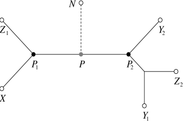
Fig. 5: This subgraph of $T$ fixes some notation used in the proof of Case 1 of Lemma 14. The location of $Y_{1}$ relative to $Y_{2}$ and $Z_{2}$ is nonessential; for instance, $Y_{1}$ can even be the same as $Y_{2}$. In $T^{*}_{k}$, ${\rm def}(P_{1})=\{X,Y_{1},Z_{1}\}$ and ${\rm def}(P_{2})=\{X,Y_{2},Z_{2}\}$. Neither $XY_{1}Z_{1}$ nor $XY_{2}Z_{2}$ is small, and $\Delta_{P_{2}Y_{2}}\leq\Delta_{P_{2}Z_{2}}$. We aim to prove that there is a leaf $N\not\in T^{*}_{k}$ such that $NXY_{2}$ or $NZ_{1}Y_{2}$ is large and defines a node $P$ strictly between $P_{1}$ and $P_{2}$ in $T$.

Lemma 14.

Assume that $P_{1}P_{2}$ is an edge in $T^{*}_{k}$ and some node is strictly between $P_{1}$ and $P_{2}$ in $T$. Then there is a large triplet $NQ_{1}Q_{2}$ with center $P$ such that $N\not\in T^{*}_{k}$, $Q_{1}\in{\rm def}(P_{1})$, $Q_{2}\in{\rm def}(P_{2})$, and $P$ is strictly between $P_{1}$ and $P_{2}$ in $T$.

Proof.

By Lemma 6(2), for every node $P$ strictly between $P_{1}$ and $P_{2}$ in $T$, there exists a leaf $N\not\in T^{*}_{k}$ with $\sigma_{PN}\geq(1-\alpha g)^{d+1}$. To choose $P$, there are two cases: (1) both $P_{1}$ and $P_{2}$ are internal nodes in $T^{*}_{k}$, and (2) $P_{1}$ or $P_{2}$ is a leaf in $T^{*}_{k}$.

Case 1. By Lemma 10, let ${\rm def}(P_{1})=\{X,Y_{1},Z_{1}\}$ and ${\rm def}(P_{2})=\{X,Y_{2},Z_{2}\}$. By ${\cal B}_{k}$, neither $XY_{2}Z_{2}$ nor $XY_{1}Z_{1}$ is small. To fix the notation for ${\rm def}(P_{1})$ and ${\rm def}(P_{2})$ with respect to their topological layout, we assume without loss of generality that Figure 5 or equivalently the following statements hold:

• In $T^{*}_{k}$ and thus in $T$ by ${\cal A}_{k}$, $P_{2}$ is on the paths between $P_{1}$ and $Y_{2}$, between $P_{1}$ and $Z_{2}$, and between $P_{1}$ and $Y_{1}$, respectively.

• Similarly, $P_{1}$ is on the paths between $P_{2}$ and $Z_{1}$ and between $P_{2}$ and $X$.

• $\Delta_{P_{2}Y_{2}}\leq\Delta_{P_{2}Z_{2}}$.

Both $NXY_{2}$ and $NZ_{1}Y_{2}$ define $P$, and the target triplet is one of these two for some suitable $P$. To choose $P$, we further divide Case 1 into three subcases.

Case 1a: $\sigma_{XP_{2}}<\sigma_{Y_{2}P_{2}}(1-\alpha g)$ and $\sigma_{Y_{2}P_{1}}<\sigma_{XP_{1}}(1-\alpha g)$. The target triplet is $NXY_{2}$. Since $\sigma_{XY_{2}}\leq\sqrt{\sigma_{XY_{2}}}$, by Corollary 3(3), let $P$ be a node on the path between $X$ and $Y_{2}$ in $T$ with $\sqrt{\sigma_{XY_{2}}(1-\alpha g)}\leq\sigma_{XP}\leq\sqrt{\sigma_{XY_{2}}(1-\alpha g)^{-1}}$ and thus by Lemma 1 $\sqrt{\sigma_{XY_{2}}(1-\alpha g)}\leq\sigma_{Y_{2}P}\leq\sqrt{\sigma_{XY_{2}}(1-\alpha g)^{-1}}$. By the condition of Case 1a and Lemma 1, $P$ is strictly between $P_{1}$ and $P_{2}$ in $T$. Also, by Corollary 4, $\sigma_{XY_{2}}\geq\frac{2}{3}\sigma_{XY_{2}Z_{2}}$. Thus, by Lemma 1, since $XY_{2}Z_{2}$ is not small,

$$\sigma_{NXY_{2}} = \frac{3}{\frac{1}{\sigma_{XP}\sigma_{PN}}+\frac{1}{\sigma_{Y_{2}P}\sigma_{PN}}+\frac{1}{\sigma_{XY_{2}}}}$$

$$\geq \frac{1}{\sqrt{\frac{2}{3}}\sigma_{XY_{2}Z_{2}}^{-1/2}(1-\alpha g)^{-d-3/2}+\frac{1}{2}\sigma_{XY_{2}Z_{2}}^{-1}}>\sigma_{\mathrm{lg}}.$$

So $NXY_{2}$ is as desired for Case 1a.

Case 1b: $\sigma_{XP_{2}}\geq\sigma_{Y_{2}P_{2}}(1-\alpha g)$. The target triplet is $NXY_{2}$. Let $P$ be the first node after $P_{2}$ on the path from $P_{2}$ toward $P_{1}$ in $T$. Then, $\sigma_{Y_{2}P}\geq\sigma_{Y_{2}P_{2}}(1-\alpha g)$. By Corollary 4, $\sigma_{Y_{2}P}^{2}\geq\sigma_{XY_{2}Z_{2}}(1-\alpha g)^{2}/3$. Next, since $\sigma_{XY_{2}}\geq\sigma_{XZ_{2}}$ and $\sigma_{P_{2}Y_{2}}\geq\sigma_{P_{2}Z_{2}}$,

$$\sigma_{XY_{2}Z_{2}}\leq\frac{3}{2\sigma_{XY_{2}}^{-1}+\sigma_{Y_{2}P_{2}}^{-1}\sigma_{P_{2}Z_{2}}^{-1}}\leq\frac{3}{2\sigma_{XP_{2}}^{-1}\sigma_{Y_{2}P_{2}}^{-1}+\sigma_{Y_{2}P_{2}}^{-2}}\leq\frac{3\sigma_{XP_{2}}^{2}}{2(1-\alpha g)+(1-\alpha g)^{2}}.$$

So $\sigma_{XP}^{2}>\sigma_{XP_{2}}^{2}>\sigma_{XY_{2}Z_{2}}(1-\alpha g)^{2}$. Since $\sigma_{XY_{2}}\geq\frac{2}{3}\sigma_{XY_{2}Z_{2}}$ and $XY_{2}Z_{2}$ is not small,

$$\sigma_{NXY_{2}} = \frac{3}{\frac{1}{\sigma_{XP}\sigma_{PN}}+\frac{1}{\sigma_{Y_{2}P}\sigma_{PN}}+\frac{1}{\sigma_{XY_{2}}}}$$

$$> \frac{1}{\left(\frac{1+\sqrt{3}}{3}\right)\sigma_{XY_{2}Z_{2}}^{-1/2}(1-\alpha g)^{-d-2}+\frac{1}{2}\sigma_{XY_{2}Z_{2}}^{-1}}>\sigma_{\mathrm{lg}}.$$

So $NXY_{2}$ is as desired for Case 1b.

Case 1c: $\sigma_{Y_{2}P_{1}}\geq\sigma_{XP_{1}}(1-\alpha g)$. If $\sigma_{Z_{1}P_{1}}>\sigma_{XP_{1}}$, the target triplet is $NZ_{1}Y_{2}$; otherwise, it is $NXY_{2}$. The two cases are symmetric, and we assume $\sigma_{XP_{1}}\geq\sigma_{Z_{1}P_{1}}$. Let $P$ be the first node after $P_{1}$ on the path from $P_{1}$ toward $P_{2}$ in $T$. Then, $\sigma_{XP}\geq\sigma_{XP_{1}}(1-\alpha g)$. By Corollary 4, $\sigma_{XP}^{2}\geq\sigma_{XP_{1}}^{2}(1-\alpha g)^{2}\geq\sigma_{XY_{1}Z_{1}}(1-\alpha g)^{2}/3$. Since $\sigma_{XY_{2}}\geq\sigma_{XZ_{2}}$ and $\sigma_{Y_{2}Z_{2}}>0$,

$$\sigma_{XY_{2}Z_{2}}\ <\ \frac{3}{2\sigma_{XY_{2}}^{-1}}\ \leq\ \frac{3}{2\sigma_{Y_{2}P_{1}}^{-1}\sigma_{XP_{1}}^{-1}}\ \leq\ \frac{3\sigma_{Y_{2}P_{1}}^{2}}{2(1-\alpha g)}.$$

Hence $\sigma_{Y_{2}P}^{2}>\sigma_{Y_{2}P_{1}}^{2}>2\sigma_{XY_{2}Z_{2}}(1-\alpha g)/3$. Then, since neither $XY_{2}Z_{2}$ nor $XY_{1}Z_{1}$ is small and $\sigma_{XY_{2}}\geq\frac{2}{3}\sigma_{XY_{2}Z_{2}}$,

$$\sigma_{NXY_{2}}=\frac{3}{\frac{1}{\sigma_{XP}\sigma_{PN}}+\frac{1}{\sigma_{Y_{2}P}\sigma_{PN}}+\frac{1}{\sigma_{XY_{2}}}}$$

$$> \frac{1}{\frac{1}{\sqrt{3}}\sigma_{XY_{1}Z_{1}}^{-1/2}(1-\alpha g)^{-d-2}+\frac{1}{\sqrt{6}}\sigma_{XY_{2}Z_{2}}^{-1/2}(1-\alpha g)^{-d-3/2}+\frac{1}{2}\sigma_{XY_{2}Z_{2}}^{-1}}>\sigma_{\mathrm{lg}}.$$

So $NXY_{2}$ is as desired for Case 1c with $\sigma_{XP_{1}}\geq\sigma_{Z_{1}P_{1}}$.

Case 2. By symmetry, assume that $P_{2}=X$ is a leaf in $T^{*}_{k}$. Since $k\geq 3$, $P_{1}$ is an internal node in $T^{*}_{k}$. Let ${\rm def}(P_{1})=\{X,Y,Z\}$. By symmetry, further assume $\sigma_{YP_{1}}\geq\sigma_{ZP_{1}}$. There are two subcases. If $\sigma_{XP_{1}}<\sigma_{YP_{1}}(1-\alpha g)$, the proof is similar to that of Case 1a and the desired $P$ is in the middle of the path between $X$ and $Y$ in $T$. Otherwise, the proof is similar that of Case 1b and $P$ is the first node after $P_{1}$ on the path from $P_{1}$ toward $X$ in $T$. In both cases, the desired triplet is $NXY$. ∎

3.4 The sample size required by Fast-HGT

The next lemma analyzes ${\cal S}$. For $k=3,\ldots,n-1$ and each leaf $M\in T$, let ${\cal S}_{k}[M]$ be the version of ${\cal S}[M]$ at the start of the $(k-2)$-th iteration of the repeat at line F7.

Lemma 15.

Assume that for a given $k\leq n-1$,  ${\cal E}_{\rm g}$, ${\cal E}_{\rm c}$, ${\cal A}_{k^{\prime}}$, ${\cal B}_{k^{\prime}}$, and ${\cal C}_{k^{\prime}}$ hold for all $k^{\prime}\leq k$.

1. If ${\cal S}_{k}[M]$ is not null, then it is a splitting tuple for some edge in $T^{*}_{k}$.

2. If an edge $Q_{1}Q_{2}\in T^{*}_{k}$ and a triplet $MR_{1}R_{2}$ with $M\not\in T^{*}_{k}$ satisfy Lemma 14, then ${\cal S}_{k}[M]$ is a splitting tuple for $Q_{1}Q_{2}$ in $T^{*}_{k}$ that contains a triplet $MR^{\prime}_{1}R^{\prime}_{2}$ with $\hat{\sigma}_{MR^{\prime}_{1}R^{\prime}_{2}}\geq\hat{\sigma}_{MR_{1}R_{2}}$.

Proof.

The two statements are proved as follows.

Statement 1. This statement follows directly from the initialization of ${\cal S}$ at line F6, the deletions from ${\cal S}$ at line F13, and the insertions into ${\cal S}$ at lines F6 and F14.

Statement 2. The proof is by induction on $k$.

Base case: $k=3$. By ${\cal E}_{\rm c}$, ${\cal A}_{3}$, ${\cal B}_{3}$, ${\cal C}_{3}$, and Lemmas 12 and 13, $MR_{1}R_{2}$ is a splitting triplet for $Q_{1}Q_{2}$ in $T^{*}_{3}$. By the maximization in Update-${\cal S}$ at line F6, ${\cal S}[M]$ is a splitting tuple for some edge $Q^{\prime}_{1}Q^{\prime}_{2}\in T^{*}_{3}$ that contains a triplet $MR^{\prime}_{1}R^{\prime}_{2}$ with $\hat{\sigma}_{MR^{\prime}_{1}R^{\prime}_{2}}\geq\hat{\sigma}_{MR_{1}R_{2}}$. By ${\cal E}_{\rm g}$, $MR^{\prime}_{1}R^{\prime}_{2}$ is not small. By Lemmas 12 and 13, $Q^{\prime}_{1}Q^{\prime}_{2}$ is $Q_{1}Q_{2}$.

Induction hypothesis: Statement 2 holds for $k<n-1$.

Induction step. We consider how ${\cal S}_{k+1}$ is obtained from ${\cal S}_{k}$ during the $(k-2)$-th iteration of the repeat at line F7. There are two cases.

Case 1: $Q_{1}Q_{2}$ also exists in $T^{*}_{k}$. By ${\cal A}_{k}$, $Q_{1}Q_{2}$ and $MR_{1}R_{2}$ also satisfy Lemmas 12 and 13 for $T^{*}_{k}$. By the induction hypothesis, ${\cal S}_{k}[M]$ is a splitting tuple for $Q_{1}Q_{2}$ in $T^{*}_{k}$ that contains a triplet $MR^{\prime}_{1}R^{\prime}_{2}$ with $\hat{\sigma}_{MR^{\prime}_{1}R^{\prime}_{2}}\geq\hat{\sigma}_{MR_{1}R_{2}}$. Then, since $Q_{1}Q_{2}\neq P_{1}P_{2}$ and $M\not=N$ at line F13, ${\cal S}_{k}[M]$ is not reset to null. Thus, it can be changed only through replacement at line F14 by a splitting tuple for some edge $Q^{\prime}_{1}Q^{\prime}_{2}$ in $T^{*}_{k+1}$ that contains a triplet $MR^{\prime\prime}_{1}R^{\prime}_{2}$ with $\hat{\sigma}_{MR^{\prime\prime}_{1}R^{\prime\prime}_{2}}\geq\hat{\sigma}_{MR^{\prime}_{1}R^{\prime}_{2}}$. By ${\cal E}_{\rm g}$, $MR^{\prime\prime}_{1}R^{\prime\prime}_{2}$ is not small. Thus, by ${\cal E}_{\rm c}$, ${\cal A}_{k+1}$, ${\cal B}_{k+1}$, ${\cal C}_{k+1}$, and Lemmas 12 and 13, $Q^{\prime}_{1}Q^{\prime}_{2}$ is $Q_{1}Q_{2}$.

Case 2: $Q_{1}Q_{2}\not\in T^{*}_{k}$. This case is similar to the base case but uses the maximization in Update-${\cal S}$ at line F14. ∎

Lemma 16.

${\cal E}_{\rm g}$ and ${\cal E}_{\rm c}$ imply that ${\cal A}_{k}$, ${\cal B}_{k}$, and ${\cal C}_{k}$ hold for all $k=3,\ldots,n$.

Proof.

The proof is by induction on $k$.

Base case: $k=3$. By Lemma 6(2), ${\cal E}_{\rm c}$, and the greedy selection of line F1, line F3 constructs $T^{*}_{3}$ without edge lengths. Then, ${\cal A}_{3}$ holds trivially. ${\cal B}_{3}$ follows from ${\cal E}_{\rm c}$, ${\cal E}_{\rm g}$, and line F1. ${\cal C}_{3}$ follows from ${\cal B}_{3}$, ${\cal E}_{\rm c}$ and the use of Equation (7) at line F4.

Induction hypothesis: ${\cal A}_{k}$, ${\cal B}_{k}$, and ${\cal C}_{k}$ hold for some $k<n$.

Induction step. The induction step is concerned with the $(k-2)$-th iteration of the repeat at line F7. Right before this iteration, by the induction hypothesis, since $k<n$, some $N^{\prime}Q_{1}Q_{2}$ satisfies Lemma 14. Therefore, during this iteration, by ${\cal E}_{\rm c}$ and Lemmas 12, 13, and 15, ${\cal S}$ at line F8 has a splitting tuple for $T^{*}_{k}$ that contains a triplet $NXY$ with $\hat{\sigma}_{NXY}\geq\hat{\sigma}_{N^{\prime}Q_{1}Q_{2}}$. Furthermore, line F9 finds such a tuple. By ${\cal E}_{\rm g}$, $NXY$ is not small. Lines F10 and F11 create $T^{*}_{k+1}$ using this triplet. Thus, ${\cal B}_{k+1}$ follows from ${\cal B}_{k}$. By Lemmas 12 and 13, ${\cal A}_{k+1}$ follows from ${\cal A}_{k}$. ${\cal C}_{k+1}$ follows from ${\cal C}_{k}$ since the triplets involved at line S13 are not small. ∎

Theorem 17.

For any $0<\delta<1$, using sequence length

$$\ell={\cal O}\left(\frac{\log\frac{1}{\delta}+\log n}{(1-\alpha g)^{4d+8}f^{2}c^{2}}\right),$$

Fast-HGT outputs $T^{*}$ with the properties below with probability at least $1-\delta$:

1. Disregarding the edge lengths, $T^{*}=\Psi_{\rm w}(T)$.

2. For each edge $Q_{1}Q_{2}$ in $T^{*}$, $|\Delta_{Q_{1}Q_{2}}^{*}-\Delta_{Q_{1}Q_{2}}|<2\Delta_{\min}$.

Proof.

By Lemma 9, ${\rm Pr}\!\left\{\,{\overline{\cal E}_{\rm g}}\,\right\}\leq\frac{\delta}{2}$ if

$$\ell\ \geq\ \ell_{\rm g}\ \stackrel{{\scriptstyle\rm def}}{{=}}\ 210\alpha^{2}\frac{3\ln n+\ln\frac{3}{\delta}}{\sigma_{\mathrm{lg}}^{2}}.$$

Similarly, by Lemma 9, ${\rm Pr}\!\left\{\,{\overline{\cal E}_{\rm c}}\,\right\}\leq\frac{\delta}{2}$ if

$$\ell\ \geq\ \ell_{\rm c}\ \stackrel{{\scriptstyle\rm def}}{{=}}\ 81\frac{3\ln n+\ln\frac{7}{\delta}}{\sigma_{\mathrm{lg}}^{2}f^{2}c^{2}}.$$

We choose $\ell=\lceil\max\{\ell_{\rm g},\ell_{\rm c}\}\rceil$. Consequently, ${\rm Pr}\!\left\{\,{{\cal E}_{\rm g}\mbox{ and }{\cal E}_{\rm c}}\,\right\}\geq 1-\delta$. By Lemma 16, with probability at least $1-\delta$, Fast-HGT outputs $T^{*}_{n}$, and ${\cal A}_{n}$ and ${\cal C}_{n}$ hold, which correspond to the two statements of the theorem. ∎

4 Further research

We have shown that theoretically, Fast-HGT has the optimal time and space complexity as well as a polynomial sample complexity. It would be important to determine the practical performance of the algorithm by testing it extensively on empirical and simulated trees and sequences. Furthermore, as conjectured by one of the referees and some other researchers, there might be a trade-off between the time complexity and the practical performance. If this is indeed true empirically, it would be significant to quantify the trade-off analytically.

Appendix A Proofs of technical lemmas

A.1 Proof of Lemma 5

Let $h_{XY}=\frac{\hat{\sigma}_{XY}}{\sigma_{XY}}$; $h_{XZ}=\frac{\hat{\sigma}_{XZ}}{\sigma_{XZ}}$; $h_{YZ}=\frac{\hat{\sigma}_{YZ}}{\sigma_{YZ}}$. By Equations (6) and (7), and by conditioning on the events $\{h_{XZ}\leq 1-r\}$ and $\{h_{YZ}\geq 1+s\}$ for some $r,s>0$,

$${\rm Pr}\!\left\{\,{\hat{\Delta}_{XP}-\Delta_{XP}\geq\frac{-\ln(1-\epsilon)}{2}}\,\right\}={\rm Pr}\!\left\{\,{{h_{XY}h_{XZ}}\leq{h_{YZ}}(1-\epsilon)}\,\right\}$$

$$\leq {\rm Pr}\!\left\{\,{h_{XZ}\leq 1-r}\,\right\}+{\rm Pr}\!\left\{\,{h_{YZ}\geq 1+s}\,\right\}+{\rm Pr}\!\left\{\,{h_{XY}\leq(1-\epsilon)\frac{1+s}{1-r}}\,\right\}.$$

Setting $\frac{1-r}{1+s}>1-\epsilon$, by Equations (3) and (4),

$${\rm Pr}\!\left\{\,{\hat{\Delta}_{XP}-\Delta_{XP}\geq\frac{-\ln(1-\epsilon)}{2}}\,\right\}\leq$$

$$\exp\left(-\frac{2}{\alpha^{2}}\ell\sigma_{XZ}^{2}r^{2}\right)+\exp\left(-\frac{2}{\alpha^{2}}\ell\sigma_{YZ}^{2}s^{2}\right)+\exp\left(-\frac{2}{\alpha^{2}}\ell\sigma_{XY}^{2}\left(1-(1-\epsilon)\frac{1+s}{1-r}\right)^{2}\right).$$

Equating these exponential terms yields equations for $r$ and $s$. The solution for $r$ is

$$r=\frac{t-\sqrt{t^{2}-u}}{2\sigma_{XZ}\sigma_{YZ}};\ t=\sigma_{XY}\sigma_{YZ}+\sigma_{XZ}\sigma_{YZ}+(1-\epsilon)\sigma_{XY}\sigma_{XZ};\ u=4\sigma_{XY}\sigma_{YZ}^{2}\sigma_{XZ}\epsilon.$$

Using Taylor’s expansion, for $u>0$, $(t-\sqrt{t^{2}-u})^{2}>\frac{u^{2}}{4t^{2}}.$ Thus,

$$r^{2}>\frac{\epsilon^{2}}{\left(\frac{1}{\sigma_{XZ}}+\frac{1-\epsilon}{\sigma_{YZ}}+\frac{1}{\sigma_{XY}}\right)^{2}\sigma_{XZ}^{2}}>\frac{\epsilon^{2}\sigma_{XYZ}^{2}}{9\sigma_{XZ}^{2}}.$$

So ${\rm Pr}\!\left\{\,{\hat{\Delta}_{XP}-\Delta_{XP}\geq\frac{-\ln(1-\epsilon)}{2}}\,\right\}\leq 3\exp\left(-\frac{2}{\alpha^{2}}\ell\sigma_{XZ}^{2}r^{2}\right)<3\exp\left(-\frac{2}{9\alpha^{2}}\ell\sigma_{XYZ}^{2}\epsilon^{2}\right).$

A.2 Proof of Lemma 7

We use the following basic inequalities.

$$\min\left\{\frac{\hat{\sigma}_{XY}}{\sigma_{XY}},\frac{\hat{\sigma}_{XZ}}{\sigma_{XZ}},\frac{\hat{\sigma}_{YZ}}{\sigma_{YZ}}\right\}\leq\frac{\hat{\sigma}_{XYZ}}{\sigma_{XYZ}}\leq\max\left\{\frac{\hat{\sigma}_{XY}}{\sigma_{XY}},\frac{\hat{\sigma}_{XZ}}{\sigma_{XZ}},\frac{\hat{\sigma}_{YZ}}{\sigma_{YZ}}\right\};$$ (16)

$$\frac{\sigma_{XYZ}}{3}\leq\min\left\{\sigma_{XY},\sigma_{XZ},\sigma_{YZ}\right\}.$$ (17)

The proof of Equation (9) is symmetric to that of Equation (8). So we only prove the latter. Pick $\lambda\geq 1$ with $\sigma_{XYZ}=\sigma_{\mathrm{lg}}\lambda$. Without loss of generality, we assume $\min\left\{\frac{\hat{\sigma}_{XY}}{\sigma_{XY}},\frac{\hat{\sigma}_{XZ}}{\sigma_{XZ}},\frac{\hat{\sigma}_{YZ}}{\sigma_{YZ}}\right\}=\frac{\hat{\sigma}_{XY}}{\sigma_{XY}}.$ By Equations (3), (16), and (17),

$${\rm Pr}\!\left\{\,{\hat{\sigma}_{XYZ}\leq\sigma_{\mathrm{md}}}\,\right\}={\rm Pr}\!\left\{\,{\frac{\hat{\sigma}_{XYZ}}{\sigma_{XYZ}}\leq\frac{\sigma_{\mathrm{md}}}{\sigma_{\mathrm{lg}}\lambda}}\,\right\}\leq{\rm Pr}\!\left\{\,{\frac{\hat{\sigma}_{XY}}{\sigma_{XY}}\leq\frac{\sigma_{\mathrm{md}}}{\sigma_{\mathrm{lg}}\lambda}}\,\right\}$$

$$\leq \exp\left(-\frac{2}{\alpha^{2}}\ell\left(1-\frac{\sigma_{\mathrm{md}}}{\sigma_{\mathrm{lg}}\lambda}\right)^{2}\sigma_{XY}^{2}\right)\leq\exp\left(-\frac{2\left(1-\frac{\sigma_{\mathrm{md}}}{\sigma_{\mathrm{lg}}}\right)^{2}}{9\alpha^{2}}\ell\sigma_{\mathrm{lg}}^{2}\right).$$

Then, Equation (8) follows from the fact that by the choice of $\sigma_{\mathrm{md}}$,

$$\frac{2\left(1-\frac{\sigma_{\mathrm{md}}}{\sigma_{\mathrm{lg}}}\right)^{2}}{9\alpha^{2}}=\frac{(\sqrt{2}-1)^{2}}{36\alpha^{2}}.$$

A.3 Proof of Lemma 8

Since Lemma 5 can help establish only one half of the desired inequality, we split the probability on the left-hand side of Equation (11).

$${\rm Pr}\!\left\{\,{\left|\hat{\Delta}_{XP}-\Delta_{XP}\right|\geq\frac{\Delta_{\min}}{2}}\,\right\}$$

$$\leq {\rm Pr}\!\left\{\,{\hat{\Delta}_{XP}-\Delta_{XP}\geq\frac{\Delta_{\min}}{6}}\,\right\}+{\rm Pr}\!\left\{\,{\hat{\Delta}_{YP}-\Delta_{YP}\geq\frac{\Delta_{\min}}{6}}\,\right\}+$$

$${\rm Pr}\!\left\{\,{\hat{\Delta}_{XP}-\Delta_{XP}\leq-\frac{\Delta_{\min}}{2}}\,\vphantom{\hat{\Delta}_{YP}-\Delta_{YP}<\frac{\Delta_{\min}}{6}}\right|\left.\vphantom{\hat{\Delta}_{XP}-\Delta_{XP}\leq-\frac{\Delta_{\min}}{2}}{\hat{\Delta}_{YP}-\Delta_{YP}<\frac{\Delta_{\min}}{6}}\,\right\}.$$

Then, since $\hat{\Delta}_{XY}-\Delta_{XY}=(\hat{\Delta}_{XP}-\Delta_{XP})+(\hat{\Delta}_{YP}-\Delta_{YP}),$ we have

$${\rm Pr}\!\left\{\,{\hat{\Delta}_{XP}-\Delta_{XP}\leq-\frac{\Delta_{\min}}{2}}\,\vphantom{\hat{\Delta}_{YP}-\Delta_{YP}<\frac{\Delta_{\min}}{6}}\right|\left.\vphantom{\hat{\Delta}_{XP}-\Delta_{XP}\leq-\frac{\Delta_{\min}}{2}}{\hat{\Delta}_{YP}-\Delta_{YP}<\frac{\Delta_{\min}}{6}}\,\right\}$$

$$\leq {\rm Pr}\!\left\{\,{\hat{\Delta}_{XY}-\Delta_{XY}\leq-\frac{\Delta_{\min}}{3}}\,\right\}.$$

Consequently,

$${\rm Pr}\!\left\{\,{\left|\hat{\Delta}_{XP}-\Delta_{XP}\right|\geq\frac{\Delta_{\min}}{2}}\,\right\} \leq {\rm Pr}\!\left\{\,{\hat{\Delta}_{XP}-\Delta_{XP}\geq\frac{\Delta_{\min}}{6}}\,\right\}+$$

$${\rm Pr}\!\left\{\,{\hat{\Delta}_{YP}-\Delta_{YP}\geq\frac{\Delta_{\min}}{6}}\,\right\}+$$

$${\rm Pr}\!\left\{\,{\hat{\Delta}_{XY}-\Delta_{XY}\leq-\frac{\Delta_{\min}}{3}}\,\right\}.$$

By Lemma 5,

$${\rm Pr}\!\left\{\,{\hat{\Delta}_{XP}-\Delta_{XP}\geq\frac{\Delta_{\min}}{6}}\,\right\}\leq 3\exp\left(-\frac{2}{9\alpha^{2}}\ell\sigma_{XYZ}^{2}\left(1-e^{-\frac{\Delta_{\min}}{3}}\right)^{2}\right).$$

By Taylor’s expansion, $\left(1-e^{-\frac{\Delta_{\min}}{3}}\right)^{2}\geq\left(1-(1-\alpha f)^{\frac{c}{3}}\right)^{2}>\frac{c^{2}}{9}\alpha^{2}f^{2},$ and thus

$${\rm Pr}\!\left\{\,{\hat{\Delta}_{XP}-\Delta_{XP}\geq\frac{\Delta_{\min}}{6}}\,\right\}\leq 3\exp\left(-\frac{c^{2}}{81}\ell\sigma_{\mathrm{lg}}^{2}f^{2}\right).$$ (19)

By symmetry,

$${\rm Pr}\!\left\{\,{\hat{\Delta}_{YP}-\Delta_{YP}\geq\frac{\Delta_{\min}}{6}}\,\right\}\leq 3\exp\left(-\frac{c^{2}}{81}\ell\sigma_{\mathrm{lg}}^{2}f^{2}\right).$$ (20)

By Equation (4), ${\rm Pr}\!\left\{\,{\hat{\Delta}_{XY}-\Delta_{XY}\leq-\frac{\Delta_{\min}}{3}}\,\right\}\leq\exp\left(-\frac{2}{\alpha^{2}}\ell\sigma_{XY}^{2}\left(e^{\frac{\Delta_{\min}}{3}}-1\right)^{2}\right).$ From Equation (17), $\sigma_{XY}\geq\frac{\left(1-\alpha g\right)^{2d+2}}{3\sqrt{2}}.$ By Taylor’s expansion, $\left(e^{\frac{\Delta_{\min}}{3}}-1\right)^{2}\geq\left((1-\alpha f)^{-\frac{c}{3}}-1\right)^{2}>\frac{c^{2}}{9}\alpha^{2}f^{2}.$ Therefore,

$${\rm Pr}\!\left\{\,{\hat{\Delta}_{XY}-\Delta_{XY}\leq-\frac{\Delta_{\min}}{3}}\,\right\}\leq\exp\left(-\frac{c^{2}}{81}\ell\sigma_{\mathrm{lg}}^{2}f^{2}\right).$$ (21)

Lemma 8 follows from the fact that putting Equations (A.3) through (21) together, we have ${\rm Pr}\!\left\{\,{\left|\hat{\Delta}_{XY}-\Delta_{XY}\right|\geq\frac{\Delta_{\min}}{2}}\,\right\}\leq 7\exp\left(-\frac{c^{2}}{81}\ell\sigma_{\mathrm{lg}}^{2}f^{2}\right).$

References

- [1] R. Agarwala, V. Bafna, M. Farach, B. Narayanan, M. Paterson, and M. Thorup. On the approximability of numerical taxonomy fitting distances by tree metrics. SIAM Journal on Computing, 2000. To appear.
- [2] A. Ambainis, R. Desper, M. Farach, and S. Kannan. Nearly tight bounds on the learnability of evolution. In Proceedings of the 38th Annual IEEE Symposium on Foundations of Computer Science, pages 524–533, 1997.
- [3] K. Atteson. The performance of neighbor-joining algorithms of phylogeny reconstruction. Algorithmica, 25(2-3):251–278, 1999.
- [4] M. Cryan, L. A. Goldberg, and P. W. Goldberg. Evolutionary trees can be learned in polynomial time in the two-state general Markov-model. In Proceedings of the 39th Annual IEEE Symposium on Foundations of Computer Science, pages 436–445, 1998.
- [5] M. Csűrös and M. Y. Kao. Recovering evolutionary trees through harmonic greedy triplets. In Proceedings of the 10th Annual ACM-SIAM Symposium on Discrete Algorithms, pages 261–270, 1999.
- [6] M. Csuros. Reconstructing Phylogenies in Markov Models of Evolution. PhD thesis, Yale University, 2000. Co-Directors: Dana Angluin and Ming-Yang Kao.
- [7] W. H. E. Day. Computational complexity of inferring phylogenies from dissimilarity matrices. Bulletin of Mathematical Biology, 49:461–467, 1987.
- [8] W. H. E. Day, D. S. Johnson, and D. Sankoff. The computational complexity of inferring rooted phylogenies by parsimony. Mathematical Biosciences, 81:33–42, 1986.
- [9] D.-Z. Du, Y.-J. Zhang, and Q. Feng. On better heuristic for Euclidean Steiner minimum trees extended abstract. In Proceedings of the 32nd Annual IEEE Symposium on Foundations of Computer Science, pages 431–439, 1991.
- [10] P. L. Erdős, M. A. Steel, L. A. Székely, and T. J. Warnow. A few logs suffice to build (almost) all trees. I. Random Structures & Algorithms, 14(2):153–184, 1999.
- [11] P. L. Erdős, M. A. Steel, L. A. Székely, and T. J. Warnow. A few logs suffice to build (almost) all trees. II. Theoretical Computer Science, 221(1-2):77–118, 1999.
- [12] M. Farach and S. Kannan. Efficient algorithms for inverting evolution. Journal of the ACM, 46(4):437–449, 1999.
- [13] J. Felsenstein. Numerical methods for inferring evolutionary trees. The Quarterly Review of Biology, 57:379–404, 1982.
- [14] J. Felsenstein. Inferring evolutionary trees from DNA sequences. In B. Weir, editor, Statistical Analysis of DNA Sequence Data, pages 133–150. Dekker, 1983.
- [15] J. Felsenstein. Statistical inference of phylogenies. Journal of the Royal Statistical Society Series A, 146:246–272, 1983.
- [16] D. Gusfield. Algorithms on Strings, Trees, and Sequences: Computer Science and Computational Biology. Cambridge University Press, New York, NY, 1997.
- [17] W. Hoeffding. Probability inequalities for sums of bounded random variables. Journal of the American Statistical Association, 58:13–30, 1963.
- [18] D. Huson, S. Nettles, and T. Warnow. Disk-covering, a fast converging method for phylogenetic tree reconstruction. Journal of Computational Biology, 6(3):369–386, 1999.
- [19] M. J. Kearns, Y. Mansour, D. Ron, R. Rubinfeld, R. E. Schapire, and L. Sellie. On the learnability of discrete distributions (extended abstract). In Proceedings of the 26th Annual ACM Symposium on Theory of Computing, pages 273–282, 1994.
- [20] M. E. Siddall. Success of parsimony in the four-taxon case: long-branch repulsion by likelihood in the Farris zone. Cladistics, 14:209–220, 1998.
- [21] M. Steel. Recovering a tree from the leaf colourations it generates under a Markov model. Applied Mathematics Letters, 7(2):19–23, 1994.
- [22] D. L. Swofford, G. J. Olsen, P. J. Waddell, and D. M. Hillis. Phylogenetic inference. In D. M. Hillis, C. Moritz, and B. K. Mable, editors, Molecular Systematics, chapter 11, pages 407–514. Sinauer Associates, Sunderland, Ma, 2nd edition, 1996.