Automatic Termination Analysis of Programs Containing Arithmetic Predicates

Abstract

For logic programs with arithmetic predicates, showing termination is not easy, since the usual order for the integers is not well-founded. A new method, easily incorporated in the TermiLog system for automatic termination analysis, is presented for showing termination in this case.

The method consists of the following steps: First, a finite abstract domain for representing the range of integers is deduced automatically. Based on this abstraction, abstract interpretation is applied to the program. The result is a finite number of atoms abstracting answers to queries which are used to extend the technique of query-mapping pairs. For each query-mapping pair that is potentially non-terminating, a bounded (integer-valued) termination function is guessed. If traversing the pair decreases the value of the termination function, then termination is established. Simple functions often suffice for each query-mapping pair, and that gives our approach an edge over the classical approach of using a single termination function for all loops, which must inevitably be more complicated and harder to guess automatically. It is worth noting that the termination of McCarthy’s 91 function can be shown automatically using our method.

In summary, the proposed approach is based on combining a finite abstraction of the integers with the technique of the query-mapping pairs, and is essentially capable of dividing a termination proof into several cases, such that a simple termination function suffices for each case. Consequently, the whole process of proving termination can be done automatically in the framework of TermiLog and similar systems.

^a School of Mathematical Sciences
Tel-Aviv University
Tel-Aviv 69978, Israel 

^b Institute for Computer Science
The Hebrew University
Jerusalem 91904, Israel 

^c Department of Computer Science
Katholieke Universiteit Leuven
B-3001 Heverlee, Belgium 

1 Introduction

In studying termination of both pure logic programs and of real Prolog programs, we discovered that in most cases, termination of the programs we encountered depended on the following factors:

1. Simple structural recursion. This case may usually be resolved by the use of term size or list length as a norm [14, 26]. General linear norms, defined in [21], are a generalisation of these standard norms.

2. Recursion with local variables. In this case an additional preprocessing step, deriving interargument relations, is necessary [4, 8, 32, 28].

3. Pseudo-recursion. These are calls to recursively defined predicates that can be eliminated by repetitive unfolding [3, 5, 23, 31].

4. Non-logical features of Prolog. Such components of Prolog programs (assert/1, !/1, ->/2, findall/3, etc.) have historically attracted less attention. Termination w.r.t. control predicates may be found, for example, in [21]. Termination w.r.t. cut was studied in [1].

5. Numerical loops. They are the topic of this paper.

6. Non-linear loops. These are situations in which recursion is not covered by general linear norms, as defined in [21].

Termination of logic programs in the general case is undecidable (see [2] for the formal proof). However, the simple semantics of logic programs made the search for sufficient conditions for termination a challenge for the research community.

Research on the first two topics of the list above led to completely automated tools for verifying termination [12, 22], based on the use of linear norms (cf.  [6, 14, 27, 34]). These systems are powerful enough to deal with a large fraction of the programs that have appeared in the literature [3, 10, 14, 21]. Moreover, most of the examples can be proved using term-size or, less often, list-size. When other linear norms are necessary, the user is expected to provide them. For any given program, these tools either provide a termination proof, or else report that there may be cases of non-termination.

Automatic linear norm inference was studied in [15]. However, there are examples, for which (it can be proved that) no general linear norm can demonstrate termination. These examples are covered by the last two items in the list above.

In this paper we concentrate on Case 5. Our approach is suitable for automatization and may be integrated in existing systems. In Case 6 more sophisticated orderings (like recursive path ordering [16]) or non-numerical sizes should be used. These may be incorporated in the query-mapping pairs technique, as described in Section 6. The difficulty here is in discovering them automatically, though techniques can be borrowed from the term-rewriting literature.

The remainder of the paper is organized as follows: In Section 2 a motivating example is given. In Sections 3–6 the different components of the algorithm are explained and in Section 7 the complete algorithm is formulated. In Section 8 some conclusions are presented.

2 The 91 function

We start by illustrating the use of our algorithm for proving the termination of the 91 function. This deliberately contrived function was invented by John McCarthy for exploring properties of recursive programs, and is considered to be a good test case for automatic verification systems (cf. [17, 20, 24]). The treatment here is on the intuitive level. Formal details will be given in subsequent sections.

Consider the clauses:

Example 2.1.

$$\mathtt{{mc\_carthy\_91}(X,Y){\ :\!\!-\ }X>100,Y\;\;is\;\;X-10.}$$

$$\mathtt{{mc\_carthy\_91}(X,Y){\ :\!\!-\ }X\leq 100,Z\;\;is\;\;X+11,{mc\_carthy\_91}(Z,Z1),}$$

$$\hskip 116.65646pt\mathtt{{mc\_carthy\_91}(Z1,Y).}$$

and assume that a query of the form mc_carthy_91($i$,$f$) is given, that is, a query in which the first argument is bound to an integer, and the second is free. This program computes the same answers as the following one:

$$\mathtt{{mc\_carthy\_91}(X,Y){\ :\!\!-\ }X>100,Y\;\;is\;\;X-10.}$$

$$\mathtt{{mc\_carthy\_91}(X,91){\ :\!\!-\ }X\leq 100.}$$

with the same query. Note, however, that while the termination of the latter program is obvious, since there is no recursion in it, the termination of the first one is far from being trivial and a lot of effort was dedicated to find termination proofs for it ([17, 20, 24]).

Our algorithm starts off by discovering numerical arguments. This step is based on abstract interpretation, and as a result both arguments of mc_carthy_91 are proven to be numerical. Moreover, they are proven to be of integer type. The importance of knowledge of this kind and techniques for its discovery are discussed in Subsection 3.2.

The next step of the algorithm is the inference of the integer abstraction domain which will help overcome difficulties caused by the fact that the (positive and negative) integers with the usual (greater-than or less-than) order are not well-founded. Integer abstractions are derived from arithmetic comparisons in the bodies of rules. However, a simplistic approach may be insufficient and the more powerful techniques presented in Section 4 are sometimes essential. In our case the domain $\{(-\infty,89],[90,100],[101,\infty)\}$ of intervals is deduced. For the sake of convenience we denote this tripartite domain by $\{$small, med, big$\}$.

In the next step, we use abstract interpretation to describe answers to queries. This allows us to infer numerical inter-argument relations of a novel type. In Section 5 the technique for inference of constraints of this kind is presented. For our running example we get the following abstract atoms.

mc_carthy_91(big,big)	mc_carthy_91(med,med)
mc_carthy_91(big,med)	mc_carthy_91(small,med)

These abstract atoms characterise the answers of the program.

The concluding step creates query-mapping pairs in the fashion of [21]. This process uses the abstract descriptions of answers to queries and is described in Section 6. In our case, we obtain among others, the query-mapping pair having the query mc_carthy_91($i$,$f$) and the mapping presented in Figure 1. The upper nodes correspond to argument positions of the head of the recursive clause, and lower nodes—to argument positions of the second recursive subgoal in the body. Black nodes denote integer argument positions, and white nodes denote positions on which no assumption is made. The arrow denotes an increase of the first argument, in the sense that the first argument in the head is less than the first argument in the second recursive subgoal. Each set of nodes is accompanied by a set of constraints. Some are inter-argument relations of the type considered in [21]. In our example this subset is empty. The rest are constraints based on the integer abstraction domain. In this case, that set contains the constraint that the first argument is in med.

Fig. 1: Mapping for McCarthy’s 91 function

The query-mapping pair presented is circular (upper and lower nodes are the same ), but the termination tests of [12, 21] fail. Thus, a termination function must be guessed. For this loop we can use the function $100-$arg1, where arg1 denotes the first argument of the atom. The value of this function decreases while traversing the given query-mapping pair from the upper to the lower nodes. Since it is also bounded from below ($100\geq$arg1), this query-mapping pair may be traversed only finitely many times. The same holds for the other circular query-mapping pair in this case. Thus, termination is proved.

3 Logic programs containing arithmetic predicates

The algorithm we describe here would come into play only when the usual termination analysers fail to prove termination using the structural arguments of predicates. As a first step it verifies the presence of an integer loop in the program. If no integer loop is found, the possibility of non-termination is reported, meaning that the termination cannot be proved by this technique. If integer loops are found, each of them is taken into consideration. The algorithm starts by discovering integer positions in the program, proceeds with creating appropriate abstractions, based on the integer loops, and concludes by applying an extension of the query-mapping pairs technique. The formal algorithm is presented in Section 7.

3.1 Numerical and integer loops

Our notion of numerical loop is based on the predicate dependency graph (cf. [26]):

Definition 3.1.

Let $P$ be a program and let $\mathchar 5\relax$ be a strongly connected component in its predicate dependency graph. Let $S\subseteq P$ be the set of program clauses, associated with $\mathchar 5\relax$ (i.e. those clauses that have the predicates of $\mathchar 5\relax$ in their head). $S$ is called loop if there is a cycle through predicates of $\mathchar 5\relax$.

Definition 3.2.

A loop $S$ is called numerical if there exists $H{\ :\!\!-\ }B_{1},\ldots,B_{n}$ in $S$, such that for some $i$, $B_{i}\equiv\mbox{\sl Var\ }\mbox{\tt is\ }\mbox{\sl Exp}$, and either Var is equal to some argument of $H$ or Exp is an arithmetic expression involving a variable that is equal to some argument of $H$.

However, termination of numerical loops that involve numbers that are not integers often depends on the specifics of implementation and hardware, so we limit ourselves to “integer loops”, rather than all numerical loops. The following examples illustrate actual behaviour that contradicts intuition of general numerical loops—a loop that should not terminate terminates, while a loop that should terminate does not. We checked the behaviour of these examples on UNIX, with the CLP(Q,R) library [18] of SICStus Prolog [30], CLP(R) [19] and XSB [29].

Example 3.3.

Consider the following program. The goal p(1.0) terminates although we would expect it not to terminate. On the other hand the goal q(1.0) does not terminate, although we would expect it to terminate.

$$\mathtt{p(0.0){\ :\!\!-\ }!.}$$

$$\mathtt{p(X){\ :\!\!-\ }X1\;\;is\;\;X/2,\;\;p(X1).}$$

$$\mathtt{q(0.0){\ :\!\!-\ }!.}$$

$$\mathtt{q(X){\ :\!\!-\ }X1\;\;is\;\;X\;-\;0.1,\;\;q(X1).}$$

One may suggest that assuming that the program does not contain division and non-integer constants will solve the problem. The following example shows that this is not the case:

Example 3.4.

$$\mathtt{r(0).}$$

$$\mathtt{r(X){\ :\!\!-\ }X>0,\;\;X1\;\;is\;\;X-1,\;\;r(X1).}$$

The predicate r may be called with a real, non-integer argument, and then its behaviour is implementation dependent. For example, one would expect that r(0.000000001) will fail and r(0.0) will succeed. However, in SICStus Prolog both goals fail, while in CLP(R) both of them succeed!

Therefore, we limit ourselves to integer loops, that is numerical loops involving integer constants and arithmetical calculations over integers:

Definition 3.5.

A program $P$ is integer-based if, given a query such that all numbers appearing in it are integers, all subqueries that arise have this property as well.

Although this definition may seem overly restrictive we use it to avoid unnecessary complications.

Definition 3.6.

A numerical loop $S$ in a program $P$ is called an integer loop if $P$ is integer-based.

Termination of a query may depend on whether its argument is an integer, as the following example shows:

$$\mathtt{p(0).}$$

$$\mathtt{p(N){\ :\!\!-\ }N\;>\;0,\;\;N1\;\;is\;\;N\;-\;1,\;\;p(N1).}$$

$$\mathtt{p(a){\ :\!\!-\ }p(a).}$$

For this program, p($n$) for integer $n$ terminates, while p(a) does not.

So we extend our notion of query pattern. Till now a query pattern was an atom with the same predicate and arity as the query, and arguments $b$ (denoting an argument that is instantiated enough with respect to the norm) or $f$ (denoting an argument on which no assumptions are made). Here, we extend the notion to include arguments of the form $i$, denoting an argument that is an integer (or integer expression). Note that $b$ includes the possibility of $i$, in the same way that $f$ includes the possibility $b$. In the diagrams to follow we denote $i$-arguments by black nodes, $b$-arguments by gray nodes and $f$-arguments by white nodes.

Our termination analysis is always performed with respect to a given program and a query pattern. A positive response guarantees termination of every query that matches the pattern.

3.2 Discovering numerical arguments

Our analysis that will be discussed in the subsequent sections is based on the size relationships between “numerical arguments”. These are arguments that are numerical for all subqueries generated from the initial query.

The inference is done in two phases—bottom-up and top-down. Bottom-up inference is similar to type analysis (cf. [7, 11]), using the abstract domain $\{\mbox{\sl int},\mbox{\sl not\_int}\}$ and the observation that an argument may become int only if it is obtained from is/2 or is bound to an integer expression of arguments already found to be int (i.e. the abstraction of $\mbox{\sl int}+\mbox{\sl int}$ is int). Top-down inference is query driven and is similar to the “blackening” process, described in [21], only in this case the information propagated is being an integer expression instead of “instantiated enough”.

The efficiency of discovering numerical arguments may be improved by a preliminary step of guessing the numerical argument positions. The guessing is based on the knowledge that variables appearing in comparisons or is/2-atoms should be numerical. Instead of considering the whole program it is sufficient in this case to consider only clauses of predicates having clauses with the guessed arguments and clauses of predicates on which they depend. The guessing as a preliminary step becomes crucial when considering “real-world” programs that are large, while their numerical part is usually small.

4 Integer Abstraction Domain

In this subsection we present a technique that allows us to overcome the difficulties caused by the fact that the integers with the usual order are not well-founded. Given a program $P$ we introduce a finite abstraction domain, representing integers. The integer abstractions are derived from the subgoals involving integer arithmetic positions.

Let $S$ be a set of clauses in $P$, consisting of an integer loop and all the clauses for predicates on which the predicates of the integer loop depend. As a first step for defining the abstract domain we obtain the set of comparisons ${\cal C}$ for the clauses in $S$.

More formally, we consider as a comparison, an atom of the form $t_{1}\rho t_{2}$, such that $t_{1}$ and $t_{2}$ are either variables or constants and $\rho\in\{<,\leq,\geq,>\}$. Observe that we restrict ourselves only to these atoms in order to ensure the finiteness of ${\cal C}$. Note that by excluding $\not=$ and $=$ we do not limit the generality of the analysis. Indeed if $t_{1}\not=t_{2}$ appears in a clause it may be replaced by two clauses containing $t_{1}>t_{2}$ and $t_{1}<t_{2}$ instead of $t_{1}\not=t_{2}$, respectively. Similarly, if the clause contains a subgoal $t_{1}=t_{2}$, the subgoal may be replaced by two subgoals $t_{1}\geq t_{2},t_{1}\leq t_{2}$. Thus, the equalities we use in the examples to follow should be seen as a brief notation as above.

In the following subsections we present a number of techniques to infer ${\cal C}$ from the clauses of $S$.

We define ${\cal D}_{p}$ as the set of pairs $(p,c)$, for all satisfiable $c\in 2^{{\cal C}_{p}}$. Here we interpret $c\in 2^{{\cal C}_{p}}$ as a conjunction of the comparisons in $c$ and the negations of the comparisons in ${\cal C}_{p}\setminus c$. The abstraction domain ${\cal D}$ is taken as the union of the sets ${\cal D}_{p}$ for the recursive predicates $p$ in $S$. Simplifying the domain may improve the running time of the analysis, however it may make it less precise.

4.1 The simple case—collecting comparisons

The simplest way to obtain ${\cal C}$ from the clauses of $S$ is to consider the comparisons appearing in the bodies of recursive clauses and restricting integer positions in their heads.

We would like to view ${\cal C}$ as a set of comparisons of head argument positions. Therefore we assume in the simple case that $S$ is partially normalised, that is, all head integer argument positions in clauses of $S$ are occupied by distinct variables. Observe that the assumption holds for all the examples considered so far. This assumption will not be necessary with the more powerful technique presented in the next subsection.

Consider

Example 4.1.

$$\mathtt{t(X){\ :\!\!-\ }X>5,X<8,X<2,X1\;is\;X+1,X1<5,t(X1).}$$

Let t($i$) be a query pattern for the program above. In this case, the first argument of t is an integer argument. Since X1 does not appear in the head of the first clause X1<5 is not considered and, thus, ${\cal C}=\{X>5,X<8,X<2\}$. We have in this example only one predicate and the union is over the singleton set. So, ${\cal D}=\{X<2,2\leq X\leq 5,5<X<8,X\geq 8\}$.

The following example evaluates the mod function.

Example 4.2.

$$\mathtt{mod(A,B,C){\ :\!\!-\ }A\geq B,B>0,D\;is\;A-B,mod(D,B,C).}$$

$$\mathtt{mod(A,B,C){\ :\!\!-\ }A<B,A\geq 0,A=C.}$$

Here we ignore the second clause since it is not recursive. Thus, by collecting comparisons from the first clause, ${\cal C}_{\mbox{\tt mod}}=\{arg1\geq arg2,arg2>0\}$ and thus, by taking all the conjunctions of comparisons of ${\cal C}$ and their negations, we obtain ${\cal D}_{\mbox{\tt mod}}=\{(\mbox{\tt mod},\mbox{\sl arg1}\geq\mbox{\sl arg2}\;\&\;\mbox{\sl arg2}>0),(\mbox{\tt mod},\mbox{\sl arg1}\geq\mbox{\sl arg2}\;\&\;\mbox{\sl arg2}\leq 0),(\mbox{\tt mod},\mbox{\sl arg1}<\mbox{\sl arg2}\;\&\;\mbox{\sl arg2}>0),(\mbox{\tt mod},\mbox{\sl arg1}<\mbox{\sl arg2}\;\&\;\mbox{\sl arg2}\leq 0)\}$.

However, sometimes the abstract domain obtained in this way is insufficient for proving termination, and thus, should be refined. The domain may be refined by enriching the underlying set of comparisons. Possible ways to do this are using inference of comparisons instead of collecting them, or performing an unfolding, and applying the collecting or inference techniques to the unfolded program.

4.2 Inference of Comparisons

As mentioned above, sometimes the abstraction domain obtained from comparisons appearing in $S$ is insufficient. Thus, we would like to refine it. Instead of collecting comparisons, appearing in bodies of clauses, we collect certain comparisons that are implied by bodies of clauses. For example, X is Y+Z implies the constraint X=Y+Z and functor(Term,Name,Arity) implies Arity$\geq 0$.

As before, we restrict ourselves to recursive clauses (or clauses recursive predicates depend on) and comparisons that constrain integer argument positions of heads. Since a comparison that is contained in the body is implied by it, we always get a superset of the comparisons obtained by the collecting technique, presented previously. The set of comparisons inferred depends on the power of the inference engine used (e.g. CLP-techniques may be used for this purpose).

We define the abstract domain ${\cal D}$ as above. Thus, the granularity of the abstract domain also depends on the power of the inference engine.

4.3 Unfolding

Unfolding (cf. [3, 5, 23, 31]) allows us to generate a sequence of abstract domains, such that each refines the previous.

More formally, let $P$ be a program and let $H{\ :\!\!-\ }B_{1},\ldots,B_{n}$ be a recursive rule in $P$. Let $P_{1}$ be the result of unfolding an atom $B_{i}$ in $H{\ :\!\!-\ }B_{1},\ldots,B_{n}$ in $P$. Let $S_{1}$ be a set of clauses in $P_{1}$, consisting of an integer loop and the clauses of the predicates on which the integer loop predicates depend. More formally, if $S$ is an integer loop, then by using the standard notation of Apt [3] we define $S_{1}$ to be $S\cup\{H\leftarrow B|(H\leftarrow B)\in P\wedge\exists(H_{1}\leftarrow B_{1})\in S,\;\mbox{\sl s.t. }\mbox{\sl rel($H_{1}$)}\sqsupseteq\mbox{\sl rel($H$)}\}$.

Obtain ${\cal D}$ for the clauses of $S_{1}$ either by collecting comparisons from rule bodies or by inferring them, and use it as a new abstraction domain for the original program. If the algorithm still fails to prove termination, the process of unfolding can be repeated. Note, that for the cases encountered in practice at most one step of unfolding is necessary.

Example 4.3.

Unfolding mc_carthy_91(Z1,Z2) in the recursive clause we obtain a new program for the query mc_carthy_91($i$,$f$)

$$\mathtt{{mc\_carthy\_91}(X,Y){\ :\!\!-\ }X>100,\;Y\;\;is\;\;X-10.}$$

$$\mathtt{{mc\_carthy\_91}(X,Y){\ :\!\!-\ }X\leq 100,\;Z1\;\;is\;\;X+11,Z1>100,}$$

$$\mathtt{\hskip 115.63243pt\;Z2\;\;is\;\;Z1-10,{mc\_carthy\_91}(Z2,Y).}$$

$$\mathtt{{mc\_carthy\_91}(X,Y){\ :\!\!-\ }X\leq 100,\;Z1\;\;is\;\;X+11,Z1\leq 100,}$$

$$\mathtt{\hskip 115.63243ptZ3\;\;is\;\;Z1+11,{mc\_carthy\_91}(Z3,Z4),}$$

$$\mathtt{\hskip 115.63243pt{mc\_carthy\_91}(Z4,Z2),{mc\_carthy\_91}(Z2,Y).}$$

Now if we use an inference engine that is able to discover that X is Y+Z implies the constraint X=Y+Z, we obtain the following constraints on the bound head integer variable $X$ (for convenience we omit redundant ones): From the first clause we obtain $X>100$. From the second clause—$X\leq 100$, and since $X+11>100$ we get $X>89$. Similarly, from the third clause—$X\leq 89$. Thus, ${\cal C}=\{X\leq 89,X>89\wedge X\leq 100,X>100\}$ Substituting this in the definition of ${\cal D}$, and removing inconsistencies and redundancies, we obtain ${\cal D}=\{X\leq 89,X>89\wedge X\leq 100,X>100\}$.

4.4 Propagating domains

The comparisons we obtain by the techniques presented above may restrict only some subset of integer argument positions. However, for the termination proof, information on integer arguments outside of this subset may be needed. For example, as we will see shortly, in order to analyse correctly mc_carthy_91 we need to determine the domain for the second argument, while the comparisons we have constrain only the first one. Thus, we need some technique of propagating abstraction domains that we obtained for one subset of integer argument positions to another subset of integer argument positions. Clearly, this technique may be seen as a heuristic and it is inapplicable if there is no interaction between argument positions.

To capture this interaction we draw a graph for each recursive numerical predicate, that has the numerical argument positions as vertices and edges between vertices that can influence each other. In the case of mc_carthy_91 we get the graph having an edge between the first argument position and the second one.

Let $\pi$ be a permutation of the vertices of a connected component of this graph. Define $\pi{\cal D}$ to be the result of replacing each occurrence of $arg_{i}$ in ${\cal D}$ by $arg_{\pi(i)}$. Consider the Cartesian product of all abstract domains $\pi{\cal D}$ thus obtained, discarding unsatisfiable conjunctions. We will call this Cartesian product the extended domain and denote it by ${\cal E}{\cal D}$. In the case of mc_carthy_91 we get as ${\cal E}{\cal D}$ the set of elements mc_carthy_91($A$,$B$), such that $A$ and $B$ are in $\{\mbox{\sl small},\mbox{\sl med},\mbox{\sl big}\}$.

More generally, when there are arithmetic relations (e.g. $Y=X+1$) between argument positions ${\cal E}{\cal D}$ can contain new subdomains that can be inferred from those in ${\cal D}$.

5 Abstract interpretation

In this section we use the integer abstractions obtained earlier to classify, in a finite fashion, all possible answers to queries. This analysis can be skipped in simple cases (just as in TermiLog constraint inference can be skipped when not needed), but is necessary in more complicated cases, like mc_carthy_91. Most examples encountered in practice do not need this analysis.

The basic idea is as follows: define an abstraction domain and perform a bottom-up constraints inference.

The abstraction domain that should be defined is a refinement of the abstraction domain we defined in Subsection 4. There we considered only recursive clauses, since non-recursive clauses do not affect the query-mapping pairs. On the other hand, when trying to infer constraints that hold for answers of the program we should consider non-recursive clauses as well. In this way using one of the techniques presented in the previous subsection both for the recursive and the non-recursive clauses an abstraction domain $\tilde{\cal D}$ is obtained. Clearly, $\tilde{\cal D}$ is a refinement of ${\cal D}$.

Example 5.1.

For mc_carthy_91 we obtain that the elements of $\tilde{\cal D}$ are the intersections of the elements in ${\cal E}{\cal D}$ (see the end of Subsection 4.4)with the constraint in the non-recursive clause and its negation.

Example 5.2.

Continuing the mod-example we considered in Example 4.2 and considering the non-recursive clause for mod as well, we obtain by collecting comparisons that $\tilde{\cal C}=\{arg1\geq arg2,arg2>0,arg1<arg2,arg3<arg2,arg1\geq 0,arg1\leq arg3,arg1\geq arg3\}$ and, thus, $\tilde{\cal D}$ consists of all pairs $(\mbox{\tt mod},c)$ for $c$ a satisfiable element of $2^{\tilde{\cal C}}$.

Given a program $P$, let $\cal B$ be the corresponding extended Herbrand base, where we assume that arguments in numerical positions are integers. Let $T_{P}$ be the immediate consequence operator. Consider the Galois connection provided by the abstraction function $\alpha:{\cal B}\rightarrow\tilde{\cal D}$ and the concretization function $\gamma:\tilde{\cal D}\rightarrow{\cal B}$ defined as follows: The abstraction $\alpha$ of an element in ${\cal B}$ is the pair from $\tilde{\cal D}$ that characterises it. The concretization $\gamma$ of an element in $\tilde{\cal D}$ is the set of all atoms in ${\cal B}$ that satisfy it. Note that $\alpha$ and $\gamma$ form a Galois connection due to the disjointness of the elements of $\tilde{\cal D}$.

Using the Fixpoint Abstraction Theorem (cf. [13]) we get that

• $\displaystyle\hskip 20.00003pt{\alpha\left(\bigcup_{n=1}^{\infty}T_{P}^{i}(\emptyset)\right)\subseteq\bigcup_{n=1}^{\infty}(\alpha\circ T_{P}\circ\gamma)^{i}(\emptyset)}$

We will take a map $\mbox{\tt w}:\tilde{\cal D}\rightarrow\tilde{\cal D}$, that is a widening [13] of $\alpha\circ T_{P}\circ\gamma$ and compute its fixpoint. Because of the finiteness of $\tilde{\cal D}$ this fixpoint may be computed bottom-up.

The abstraction domain $\tilde{\cal D}$ describes all possible atoms in the extended Herbrand base ${\cal B}$. However, it is sufficient for our analysis to describe only computed answers of the program, i.e., a subset of ${\cal B}$. Thus, in practice, the computation of the fixpoint can sometimes be simplified as follows: We start with the constraints of the non-recursive clauses. Then we repeatedly apply the recursive clauses to the set of the constraints obtained thus far, but abstract the conclusions to elements of ${\cal D}$. In this way we obtain a CLP program that is an abstraction of the original one. This holds in the next example. The abstraction corresponding to the predicate p is denoted ${\mathtt{p_{w}}}$.

Example 5.3.

Consider once more mc_carthy_91. As claimed above we start from the non-recursive clause, and obtain that

$$\mathtt{{mc\_carthy\_91}_{w}(A,B){\ :\!\!-\ }\{A>100,B=A-10\}.}$$

By substituting in the recursive clause of mc_carthy_91 we obtain the following

$$\mathtt{{mc\_carthy\_91}(X,Y){\ :\!\!-\ }X\leq 100,\;Z1\;\;is\;\;X+11,Z1>100,}$$

$$\mathtt{\hskip 108.405pt\;Z2\;\;is\;\;Z1-10,Z2>100,\;Y\;\;is\;\;Z2-10.}$$

By simple computation we discover that in this case X is 100, and Y is 91. However, in order to guarantee the termination of the inference process we do not infer the precise constraint $\{X=100,Y=91\}$, but its abstraction, i.e., an atom $\mathtt{{mc\_carthy\_91}_{w}({med},{med})}$. Repeatedly applying the procedure described, we obtain an additional answer $\mathtt{{mc\_carthy\_91}_{w}({small},{med})}$.

More formally, the following SICStus Prolog CLP(R) program performs the bottom-up construction of the abstracted program, as described above. We use the auxiliary predicate in/2 to denote a membership in ${\cal D}$ and the auxiliary predicate e_in/2 to denote a membership in the extended domain ${\cal E}{\cal D}$.

$$\mathtt{{\ :\!\!-\ }use\_module(library(clpr)).}$$

$$\mathtt{{\ :\!\!-\ }use\_module(library(terms)).}$$

$$\mathtt{{\ :\!\!-\ }dynamic({mc\_carthy\_91}_{w}/2).}$$

$$\mathtt{in(X,big){\ :\!\!-\ }\{X>100\}.}$$

$$\mathtt{in(X,med){\ :\!\!-\ }\{X>89,X\leq 100\}.}$$

$$\mathtt{in(X,small){\ :\!\!-\ }\{X\leq 89\}.}$$

$$\mathtt{e\_in((X,Y),(XX,YY)){\ :\!\!-\ }in(X,XX),in(Y,YY).}$$

$$\mathtt{{mc\_carthy\_91}_{w}(X,Y){\ :\!\!-\ }\{X>100,Y=X-10\}.}$$

$$\mathtt{assert\_if\_new((H{\ :\!\!-\ }B)){\ :\!\!-\ }\backslash\!+(clause(H1,B1),}$$

$$\mathtt{\hskip 170.71652ptunify\_with\_occurs\_check((H,B),(H1,B1))),}$$

$$\mathtt{\hskip 147.95424ptassert((H{\ :\!\!-\ }B)).}$$

$$\mathtt{deduce{\ :\!\!-\ }\{X\leq 100,Z=X+11\},{mc\_carthy\_91}_{w}(Z,Z1),}$$

$$\mathtt{\hskip 56.9055pt{mc\_carthy\_91}_{w}(Z1,Y),e\_in((X,Y),(XX,YY)),}$$

$$\mathtt{\hskip 56.9055ptassert\_if\_new(({mc\_carthy\_91}_{w}(A,B){\ :\!\!-\ }e\_in((A,B),(XX,YY)))),}$$

$$\mathtt{\hskip 56.9055ptdeduce.}$$

$$\mathtt{deduce.}$$

The resulting abstracted program is

$$\mathtt{{mc\_carthy\_91}_{w}(A,B){\ :\!\!-\ }\{A>100,B=A-10\}.}$$

$$\mathtt{{mc\_carthy\_91}_{w}(A,B){\ :\!\!-\ }e\_in((A,B),(med,med)).}$$

$$\mathtt{{mc\_carthy\_91}_{w}(A,B){\ :\!\!-\ }e\_in((A,B),(small,med)).}$$

Since we assumed that the query was of the form mc_carthy_91($i$,$f$) we can view these abstractions as implications of constraints like $\mbox{\sl arg1}\leq 89$ implies $89<\mbox{\sl arg2}\leq 100$. We also point out that the resulting abstracted program coincides with the results obtained by the theoretic reasoning above.

As an additional example consider the computation of the gcd according to Euclid’s algorithm. Proving termination is not trivial, even if the successor notation is used. In [23] only applying a special technique allowed to do this.

Example 5.4.

Consider the following program and the query gcd($i$,$i$,$f$).

$$\mathtt{gcd(X,0,X){\ :\!\!-\ }X>0.}$$

$$\mathtt{gcd(X,Y,Z){\ :\!\!-\ }Y>0,mod(X,Y,U),gcd(Y,U,Z).}$$

$$\mathtt{mod(A,B,C){\ :\!\!-\ }A\geq B,B>0,D\;is\;A-B,mod(D,B,C).}$$

$$\mathtt{mod(A,B,C){\ :\!\!-\ }A<B,A\geq 0,A=C.}$$

In this example we have two nested integer loops represented by the predicates mod and gcd. We would like to use the information obtained from the abstract interpretation of mod to find the relation between the gcd-atoms in the recursive clause. Thus, during the bottom-up inference process we abstract the conclusions to elements of ${\tilde{\cal D}_{\mathtt{m}od}}$, as it was evaluated in Example 5.2. Using this technique we get that if $mod(X,Y,Z)$ holds then always $Z<Y$ holds, and this is what is needed to prove the termination of $gcd$.

The approach presented in this subsection is a novel approach compared to the inter-argument relations that were used previously in termination analysis [4, 9, 12, 14, 21, 25, 26, 32, 33, 34]—instead of comparing the sizes of arguments the “if …then …” expressions are considered, making the analysis more powerful.

6 Query-mapping pairs

We use the query-mapping pairs technique, presented in [21], for reasoning about termination. The basic idea is to partition query evaluation into “simple steps”, corresponding to one rule application and then compose them. The “steps” are performed over a finite abstract domain. Circular “steps” are suspicious. If, for each such circular step, we succeed in showing a decrease of some argument position according to some integer linear norm, termination is proved, due to the well-foundedness of the norm. Since the abstract domain is finite, we have to check only a finite number of objects. Here, we extend the technique to programs having numerical arguments. We also assume that an integer linear norm is defined for all arguments.

As presented in [21], queries are given as constrained abstract atoms. More formally, let $\leftarrow A_{1},\ldots,A_{n}\leadsto\ldots\leadsto\;\leftarrow B_{1},\ldots,B_{k}$ be a partial branch in the LD-tree [3], and let $\theta$ be the composition of the substitutions along this branch. Assume also that the atom $B_{1}$ came into being from the resolution on $A_{1}$. In the query-mapping pair corresponding to this branch, the query is the abstraction of $A_{1}$ and the mapping is a quadruple—the domain, the range, arcs and edges. The domain is the abstraction of $A_{1}\theta$, the range is the abstraction of $B_{1}$ and arcs and edges represent order relations between the nodes of the domain and range. Note that edges are undirected, while arcs are directed.

We extend this construction by adding numerical arcs and edges between numerical argument positions. These arcs and edges are added if numerical inequalities and equalities between the arguments can be deduced. Deduction of numerical edges and arcs is usually done by considering the clauses. However, if a subquery $q$ unifies with a head of a clause $A{\ :\!\!-\ }B_{1},\ldots,B_{k},\ldots,B_{n}$ and we want to know the relation between $q$ and $B_{k}$ (under appropriate substitutions), we may use the results of the abstract interpretation to conclude numerical constraints for $B_{1},\ldots,B_{k-1}$. The reason is that if we arrive at $B_{k}$, this means that we have proved $B_{1},\ldots,B_{k-1}$ (under appropriate substitutions). All query-mapping pairs deduced in this way are then repeatedly composed. The process terminates because there is a finite number of query-mapping pairs.

A query-mapping pair is called circular if the query coincides with the range. The initial query terminates if for every circular query-mapping pair one of the following conditions holds:

• The circular pair meets the requirements of the termination test of [21].

• There is a non-negative termination function for which we can prove a decrease from the domain to the range using the numerical edges and arcs and the constraints of the domain and range.

Two points should be referred to: how does one automate the guessing of the function ? And how does one prove that it decreases? Our heuristic for guessing a termination function is based on the inequalities appearing in the abstract constraints. Each inequality of the form Exp1$\;\rho\;$Exp2 where $\rho$ is one of $\{>,\geq\}$ suggests a function Exp1-Exp2.

The common approach to termination analysis is to find one termination function that decreases over all possible execution paths. This leads to complicated termination functions. Our approach allows one to guess a number of relatively simple termination functions, each suited to its query-mapping pair. Since termination functions are simple to find, the guessing process can be performed automatically.

After the termination function is guessed, its decrease must be proved. Let $V_{1},\ldots,V_{n}$ denote numerical argument positions in the domain and $U_{1},\ldots,U_{n}$ the corresponding numerical argument positions in the range of the query-mapping pair. First, edges of the query-mapping pair are translated to equalities and arcs, to inequalities between these variables. Second, the atom constraints for the $V$’s and for the $U$’s are added. Third, let $\varphi$ be a termination function. We would like to check that $\varphi(V_{1},\ldots,V_{n})>\varphi(U_{1},\ldots,U_{n})$ is implied by the constraints. Thus, we add the negation of this claim to the collection of the constraints and check for unsatisfiability. Since termination functions are linear, CLP-techniques, such as CLP(R) [19] and CLP(Q,R) [18], are robust enough to obtain the desired contradiction. Note however, that if more powerful constraints solvers are used, non-linear termination functions may be considered.

To be more concrete:

Example 6.1.

Consider the following program with query p($i$,$i$).

$$\mathtt{p(0,\_).}$$

$$\mathtt{p(X,Y){\ :\!\!-\ }X>0,X<Y,X1\;\;is\;\;X+1,p(X1,Y).}$$

$$\mathtt{p(X,Y){\ :\!\!-\ }X>0,X\geq Y,X1\;\;is\;\;X-5,Y1\;\;is\;\;Y-1,p(X1,Y1).}$$

We get, among others, the circular query-mapping pair having the query (p($i$,$i$),$\{\mbox{\sl arg1}>0,\mbox{\sl arg1}<\mbox{\sl arg2}\}$) and the mapping given in Figure 2. The termination function derived for the circular query-mapping pair is arg2$-$arg1. In this case, we get from the arc and the edge the constraints: $V_{1}<U_{1},V_{2}=U_{2}$. We also have that $V_{1}>0,U_{1}>0,V_{1}<V_{2},U_{1}<U_{2}$. We would like to prove that $V_{2}-V_{1}>U_{2}-U_{1}$ is implied. Thus, we add $V_{2}-V_{1}\leq U_{2}-U_{1}$ to the set of constraints and CLP-tools easily prove unsatisfiability, and thus, that the required implication holds.

Fig. 2: Mapping for p

In the case of the 91-function the mappings are given in Figure 3. (We omit the queries from the query-mapping pairs, since they are identical to the corresponding domains.)

Fig. 3: Mappings for McCarthy’s 91 function

In the examples above there were no interargument relations of the type considered in [21]. However, this need not be the case in general. Consider the following program with the query q($b$,$b$,$i$).

$$(1) \mathtt{q(s(X),X,\_).}$$

$$(2) \mathtt{q(s(X),X,N){\ :\!\!-\ }N>0,N1\;\;is\;\;N-1,q(s(X),X,N1).}$$

$$(3) \mathtt{q(s(s(X)),Z,N){\ :\!\!-\ }N=<0,N1\;\;is\;\;N-1,q(s(X),Y,N1),q(Y,Z,N1).}$$

Note that constraint inference is an essential step for proving termination—in order to infer that there is a decrease in the first argument between the head of (3) and the second recursive call ($s(s(X))\succ Y$ with respect to the norm), one should infer that the second argument in q is less than the first with respect to the norm ($s(X)\succ Y$ with respect to the norm). We get among others circular query-mapping pairs having the mappings presented in Figure 4. The queries of the mappings coincide with the corresponding domains. In the first mapping termination follows from the decrease in the third argument and the termination function arg3$>0$. In the second mapping termination follows from the norm decrease in the first argument.

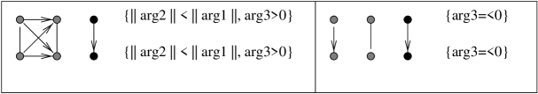
Fig. 4: Mappings for q

7 The Algorithm

In this section we combine all the techniques suggested so far. The complete algorithm Analyse_Termination is presented in Figure 5. We use the common notation of continue as a keyword, that can be used only in the body of a looping command and invokes skipping to the next iteration of the loop. Each step of the algorithm corresponds to one of the previous sections.

Algorithm Analyse_Termination Input A query pattern $q$ and a Prolog program $P$ Output YES, if termination is guaranteed NO, if no termination proof was found (1) If TermiLog_Algorithm($P$,$q$)=YES then (2) Return YES. (3) If there is no numerical loop in $P$ then (4) Return NO. (5) Guess and verify numerical argument positions; (6) Compute integer abstraction domain; (7) Compute abstractions of answers to queries (optional); (8) Compute query-mapping pairs; (9) For each circular query-mapping pair do: (10) If its circular variant has a forward positive cycle then (11) Continue; (12) Guess bounded (integer-valued) termination function; (13) Traverse the query-mapping pair and compute values of the termination function; (14) If the termination function decreases monotonically then (15) Continue; (16) Return NO; (17) Return YES.

Fig. 5: Termination Analysis Algorithm

Note that Step 7, computing the abstractions of answers to queries, is optional. If the algorithm returns NO it may be re-run either with Step 7 included or with a different integer abstraction domain.

The Analyse_Termination algorithm is sound:

Theorem 7.1.

Let $P$ be a program and $q$ a query pattern.

• Analyse_Termination($P$, $q$) terminates.

• If Analyse_Termination($P$, $q$) reports YES then, for every query $Q$ matching the pattern $q$, the LD-tree of $Q$ w.r.t. $P$ is finite.

8 Conclusion

We have shown an approach that can extend the scope of existing automatic systems for proving termination to programs containing arithmetic predicates. To do so we first introduced a new kind of constraints. Second, we indicated how such constraints may be inferred. Finally, we showed that the query-mapping pairs technique is robust enough to incorporate them by using very simple termination functions that are derived from the constraints.

We have not yet implemented the ideas discussed in this paper, but it is clear that even a simple implementation, without inference of comparisons, unfolding and application of abstract interpretation as suggested in Section 5, will be very useful from a practical point of view, since many programs encountered in practice cannot be handled by systems that use norms to prove termination because of very simple numerical loops.

References

-
[1]
J. H. Andrews.
Termination Semantics of Logic Programs with Cut and
Related Features.
Available at
http://www.inferenzsysteme.informatik.tu-darmstadt.de/~giesl/WST99/submissions/andrews.ps, May 1999. - [2] K. R. Apt. Logic programming. In J. van Leeuwen, editor, Handbook of Theoretical Computer Science, volume B: Formal Models and Semantics, chapter 15, pages 493–574. MIT Press, 1990.
- [3] K. R. Apt. From Logic Programming to Prolog. Prentice-Hall International Series in Computer Science. Prentice Hall, 1997.
- [4] F. Benoy and A. King. Inferring argument size relationships with CLP(R). In J. Gallagher, editor, Logic Program Synthesis and Transformation. Proceedings, pages 204–223. Springer Verlag, 1996. Lecture Notes in Computer Science, volume 1207.
- [5] A. Bossi and N. Cocco. Preserving universal temination through unfold/fold. In G. Levi and M. Rodríguez-Artalejo, editors, Algebraic and Logic Programming, pages 269–286. Springer Verlag, 1994. Lecture Notes in Computer Science, volume 850.
- [6] A. Bossi, N. Cocco, and M. Fabris. Norms on terms and their use in proving universal termination of a logic program. Theoretical Computer Science, 124(2):297–328, February 1994.
- [7] J. Boye and J. Małuszyński. Directional types and the annotation method. Journal of Logic Programming, 33(3):179–220, 1997.
- [8] A. Brodsky and Y. Sagiv. Inference of monotonicity constraints in datalog programs. In Proceedings of the Eighth ACM SIGACT-SIGART-SIGMOD Symposium on Principles of Database Systems, pages 190–199, 1989.
- [9] A. Brodsky and Y. Sagiv. Inference of inequality constraints in logic programs. In Proceedings of the Tenth ACM SIGACT-SIGART-SIGMOD Symposium on Principles of Database Systems, pages 227–240, 1991.
- [10] F. Bueno, M. J. García de la Banda, and M. V. Hermenegildo. Effectiveness of global analysis in strict independence-based automatic parallelization. In M. Bruynooghe, editor, Logic Programming, Proceedings of the 1994 International Symposium, pages 320–336. MIT Press, 1994.
- [11] M. Codish and V. Lagoon. Type dependencies for logic programs using ACI-unification. In Proceedings of the 1996 Israeli Symposium on Theory of Computing and Systems, pages 136–145. IEEE Press, June 1996.
- [12] M. Codish and C. Taboch. A semantic basis for termination analysis of logic programs. The Journal of Logic Programming, 41(1):103–123, 1999.
- [13] P. Cousot and R. Cousot. Abstract interpretation and application to logic programs. The Journal of Logic Programming, 13:103–180, 1992.
- [14] D. De Schreye and S. Decorte. Termination of logic programs: The never-ending story. The Journal of Logic Programming, 19/20:199–260, May/July 1994.
- [15] S. Decorte and D. De Schreye. Demand-driven and constraint-based automatic left termination analysis for logic programs. In L. Naish, editor, Proceedings of the Fourteenth International Conference on Logic Programming, pages 78–92. MIT Press, July 1997.
- [16] N. Dershowitz. Orderings for term-rewriting systems. Theoretical Computer Science, 17(3):279–301, 1982.
- [17] J. Giesl. Termination of nested and mutually recursive algorithms. Journal of Automated Reasoning, 19:1–29, 1997.
- [18] C. Holzbaur. OFAI CLP(Q,R) Manual. Technical Report TR-95-09, Austrian Research Institute for Artificial Intelligence, Vienna, 1995.
- [19] J. Jaffar and M. J. Maher. Constraint logic programming: A survey. The Journal of Logic Programming, 19/20:503–582, May/July 1994.
- [20] D. E. Knuth. Textbook examples of recursion. In V. Lifschitz, editor, Artificial Intelligence and Mathematical Theory of Computation. Papers in Honor of John McCarthy, pages 207–229. Academic Press, Inc., 1991.
- [21] N. Lindenstrauss and Y. Sagiv. Automatic termination analysis of logic programs. In L. Naish, editor, Proceedings of the Fourteenth International Conference on Logic Programming, pages 63–77. MIT Press, July 1997.
- [22] N. Lindenstrauss, Y. Sagiv, and A. Serebrenik. TermiLog: A system for checking termination of queries to logic programs. In O. Grumberg, editor, Computer Aided Verification, 9th International Conference, pages 63–77. Springer Verlag, June 1997. Lecture Notes in Computer Science, volume 1254.
- [23] N. Lindenstrauss, Y. Sagiv, and A. Serebrenik. Unfolding mystery of the mergesort. In N. Fuchs, editor, Proceedings of the Seventh International Workshop on Logic Program Synthesis and Transformation. Springer Verlag, 1998. Lecture Notes in Computer Science, volume 1463.
- [24] Z. Manna and J. McCarthy. Properties of Programs and partial function logic. Machine Intelligence, 5:27–37, 1970.
- [25] F. Mesnard and J. Ganascia. CLP(Q) for proving interargument relations. In A. Petrossi, editor, Proceedings META’92, pages 309–320. Springer Verlag, 1992.
- [26] L. Plümer. Termination Proofs for Logic Programs. Lecture Notes in Artificial Intelligence, volume 446. Springer Verlag, 1990.
- [27] L. Plümer. Termination proofs for logic programs based on predicate inequalities. In Proceedings of ICLP’90, pages 634–648. MIT Press, 1990.
- [28] L. Plümer. Automatic termination proofs for prolog programs operating on nonground terms. In International Logic Programming Symposium. MIT Press, 1991.
- [29] K. F. Sagonas, T. Swift, and D. S. Warren. The XSB Programmer’s Manual. Version 1.3 (). Department of Computer Science, SUNY @ Stony Brook, U.S.A., September 1993.
- [30] SICS. User Manual. Version 3.7.1. Swedish Institute of Computer Science, 1998.
- [31] H. Tamaki and T. Sato. Unfold/Fold transformation of logic programs. In S.-Å. Tärnlund, editor, Proceedings of the Second International Logic Programming Conference, pages 127–138. Uppsala University, 1984.
- [32] J. D. Ullman and A. van Gelder. Efficient tests for top-down termination of logical rules. Journal of the Association for Computing Machinery, 35(2):345–373, April 1988.
- [33] K. Verschaetse and D. De Schreye. Deriving termination proofs for logic programs, using abstract procedures. In K. Furukawa, editor, Logic Programming, Proceedings of the Eigth International Conference, pages 301–315. MIT Press, 1991.
- [34] K. Verschaetse and D. De Schreye. Deriving of linear size relations by abstract interpretation. In M. Bryunooghe and M. Wirsing, editors, Programming Language Implementation and Logic Programming, 4th International Symposium, pages 296–310. Springer Verlag, 1992. Lecture Notes in Computer Science, volume 631.