Optimal Buy-and-Hold Strategies for Financial Markets with Bounded Daily Returns

Abstract

In the context of investment analysis, we formulate an abstract online computing problem called a planning game and develop general tools for solving such a game. We then use the tools to investigate a practical buy-and-hold trading problem faced by long-term investors in stocks. We obtain the unique optimal static online algorithm for the problem and determine its exact competitive ratio. We also compare this algorithm with the popular dollar averaging strategy using actual market data.

1 Introduction

In an online problem, an online algorithm ${\cal B}$ is given one input at a time from a sequence of inputs. ${\cal B}$ takes an action on each input before seeing any remaining input. In contrast, an off-line algorithm sees the entire input sequence before it takes any action. Each action yields a positive accumulation. Let $E$ denote the set of all admissible input sequences. Let ${\cal C}(\vec{e})$ denote the (expected) total accumulation of an online or offline algorithm ${\cal C}$ on $\vec{e}\in E$. Let ${\cal A}$ denote the optimal offline algorithm, i.e., one that produces the largest total accumulation on each admissible input sequence. In competitive analysis [25, 27, 4], ${\cal B}$’s performance is measured by its competitive ratio

$$\Upsilon_{\cal B} = \sup_{\vec{e}\in E}\frac{{\cal A}(\vec{e})}{{\cal B}(\vec{e})}.$$ (1)

The online player seeks to minimize this ratio by choosing a suitable ${\cal B}$ while the adversary attempts to maximize it by picking $\vec{e}$ after examining ${\cal B}$. This paper assumes that the adversary is oblivious, i.e., it fixes the input sequence before ${\cal B}$ performs any computation such as generating random bits.

A planning game is an abstract online problem where the length of the input sequence is fixed and known a priori to ${\cal B}$. This time horizon feature captures many important online problems including those for portfolio rebalancing [8, 7, 21], asset trading [2, 5, 11, 12], secretary selection [1, 6, 13, 16], and bipartite matching [15, 17]. A planning game is finite if the numbers of admissible sequences of actions and inputs are both finite; otherwise, it is infinite. A finite planning game corresponds to a linear programming problem, where an optimal randomized online algorithm corresponds to an optimal feasible solution. Consequently, we can show that the smallest competitive ratio of any randomized online algorithm for such a game is the reciprocal of the value of the game as a zero-sum two-person game.

In this general optimization framework, we investigate the buy-and-hold trading problem defined as follows. An investor starts with some capital, which is normalized to $1$ dollar, and trades it for a certain security over $n$ days, which is referred to as the investment horizon. To avoid triviality, we assume $n\geq 2$. On each day, the security has only one exchange rate, i.e., the number of shares of the security which one unit of capital can buy. Upon seeing the exchange rate, the investor executes one transaction for that day and may trade all or part of the remaining capital. All the capital must be traded by the $n$-th day, and converting the acquired security back to capital is prohibited. The total accumulation of the investor is the number of shares of the security she accumulates at the end of the investment horizon. Note that the competitive ratio between the adversary’s and the investor’s accumulations is exactly the competitive ratio between the dollar values of the accumulations. This problem is faced by millions of investors who save for retirement purposes on a long-term basis; for instance, a widely popular security for today’s investors would be a stock index fund.

We employ the bounded daily return model, in which the next day’s exchange rate $e^{\prime}$ depends on the current day’s exchange rate $e$ with $e/\beta\leq e^{\prime}\leq e\alpha$ for some fixed $\alpha,\beta>1$. The values $n$, $\alpha$, and $1/\beta$ are known a priori to the investor. We call $\alpha$ and $1/\beta$ the daily return bounds. Figure 1 gives some stock markets which enforce such ratios through circuit breakers. This model can also be regarded as an approximation to the geometric Brownian motion model used extensively in the finance community [14, 20, 18, 24, 26, 3, 9].

Exchange	Circuit Breaker
	$\alpha^{-1}$	$\beta$
Amsterdam	$90\%$	$110\%$
Bangkok	$90\%$	$110\%$
Paris	$95\%$	$110\%$
Taipei	$93\%$	$107\%$
Tel-Aviv	$95\%$	$110\%$
Tokyo	$95\%$	$130\%$
Vienna	$95\%$	$105\%$

Fig. 1: Circuit breaker rules in various exchanges.

A static algorithm is an online algorithm for the buy-and-hold trading problem such that for $1\leq i\leq n$, the (expected) amount of dollars invested by the algorithm on the $i$-th day is the same for all exchange rate sequences. A dynamic algorithm refers to any online algorithm for the problem, which is not necessarily static. The static buy-and-hold trading problem refers to the case of the problem where the investor can only use a static algorithm.

We prove that the smallest possible competitive ratio for any randomized or deterministic static algorithm is $\frac{n\alpha\beta-(n-1)(\alpha+\beta)+(n-2)}{\alpha\beta-1}$. We also obtain a deterministic static algorithm with this competitive ratio, called the balanced strategy, and prove that it is the only optimal deterministic static algorithm. In comparison, the popular dollar averaging strategy has a strictly greater competitive ratio and thus is not optimal. The balanced strategy is so simple that it can be executed even by those who are not mathematically sophisticated. Starting with one dollar initially, the algorithm invests $\frac{\alpha(\beta-1)}{n\alpha\beta-(n-1)(\alpha+\beta)+(n-2)}$ dollar on the first day, $\frac{(\alpha-1)\beta}{n\alpha\beta-(n-1)(\alpha+\beta)+(n-2)}$ dollar on the last day, and $\frac{(\alpha-1)(\beta-1)}{n\alpha\beta-(n-1)(\alpha+\beta)+(n-2)}$ dollar on each of the other days.

Previously, El-Yaniv et al [11, 10, 12] obtained optimal online algorithms for this unidirectional trading problem under the assumption that the daily exchange rates, instead of the daily returns, are between a pair of upper and lower bounds. Al-Binali [2] further studied the same setting in a framework of risk and reward [19]. Our model and that of El-Yaniv et al are each formulated for real but different regulations of stock and foreign currency markets. A subtle difference between these models is that their model fixes a upper bound and a lower bound on the daily exchange rates globally for the entire investment horizon, while our model sets new bounds dynamically every day. Interestingly, although this difference might seem minor, they give rise to mathematical results of very distinct flavors using significantly different techniques.

Section 2 discusses how to compute optimal randomized online algorithms for finite planning games. Section 3 uses the general analysis in §2 to derive the balanced strategy and compare it with the dollar averaging strategy. Section 4 concludes the paper with some open problems.

2 General analysis of finite planning games

A finite planning game $G$ can be regarded as a finite zero-sum two-person game $\Gamma_{H}(m,n)$ defined as follows. For any integer $k>0$, let $Z_{k}=\{1,2,\ldots,k\}$. The maximizing player is the online player, whose pure strategies are the deterministic online algorithms ${\cal B}_{i}$ of $G$ indexed with $i\in Z_{m}$. The minimizing player is the adversary of $G$, whose pure strategies are the input sequences $\vec{\sigma}_{j}$ of $G$ indexed with $j\in Z_{n}$. The payoff matrix $H$ of $\Gamma_{H}(m,n)$ is defined by

$$H(i,j)=\frac{{\cal B}_{i}(\vec{\sigma}_{j})}{{\cal A}(\vec{\sigma}_{j})}>0,\quad i\in Z_{m}\ \mbox{and}\ j\in Z_{n}.$$ (2)

Let $\Phi(Z_{k})$ be the set of all probability density functions defined on $Z_{k}$. For $k=n$ or $m$, each $h\in\Phi(Z_{k})$ is regarded as a point in the $k$-dimensional Euclidean space and represents a mixed strategy that applies the $\ell$-th pure strategy indexed by $Z_{k}$ with probability $h(\ell)$. By von Neumann’s minimax theorem [22],

$$\max_{f\in\Phi(Z_{m})}\min_{g\in\Phi(Z_{n})}\sum_{i=1}^{m}\sum_{j=1}^{n}f(i)g(j)H(i,j) = \min_{g\in\Phi(Z_{n})}\max_{f\in\Phi(Z_{m})}\sum_{i=1}^{m}\sum_{j=1}^{n}f(i)g(j)H(i,j)$$

$$= \max_{f\in\Phi(Z_{m})}\min_{j\in Z_{n}}\sum_{i=1}^{m}f(i)H(i,j)$$

$$= \min_{g\in\Phi(Z_{n})}\max_{i\in Z_{m}}\sum_{j=1}^{n}g(j)H(i,j),$$

which is called the value $v^{*}$ of $\Gamma_{H}(m,n)$.

Let $r^{*}$ be the smallest possible competitive ratio of any randomized online algorithm for $G$; i.e.,

$$r^{*}=\min_{f\in\Phi(Z_{m})}\max_{j\in Z_{n}}\frac{{\cal A}(\vec{\sigma}_{j})}{\sum_{i=1}^{m}f(i){\cal B}_{i}(\vec{\sigma}_{j})}.$$

A randomized online algorithm is optimal if its competitive ratio is $r^{*}$.

The next theorem relates $G$ and $\Gamma_{H}(m,n)$.

Theorem 1.

1. $r^{*}=\frac{1}{v^{*}}.$

2. An optimal mixed strategy of the online player of $\Gamma_{H}(m,n)$ induces an optimal randomized online algorithm for $G$, and vice versa.

Proof.

This theorem follows from Equation (2). ∎

In light of Theorem 1, we use $G$ and $\Gamma_{H}(m,n)$ interchangeably. A main purpose of this paper is to derive the exact value of $r^{*}$ and an optimal randomized online algorithm for $G$. To do so by means of Theorem 1, the primal and dual problems of $\Gamma_{H}(m,n)$ or $G$ are defined as follows:

Primal:				Dual:
minimize	$x^{T}u_{m}$			maximize	$y^{T}u_{n}$
subject to	$x^{T}H\geq u_{n}^{T}$			subject to	$Hy\leq u_{m}$
	$x\geq 0$				$y\geq 0$

where $u_{k}$ is the column vector of $k$ copies of 1.

For each $j\in Z_{n}$, let $H^{j}$ denote the $j$-th column of $H$. Moreover, let $X$ and $Y$ be the sets of feasible solutions to the primal and dual problems of $G$, respectively. Let $\bar{X}$ and $\bar{Y}$ be the sets of optimal feasible solutions to these problems. Let $X^{*}$ and $Y^{*}$ be the sets of optimal mixed strategies of the online player and the adversary, respectively.

The next lemma is useful for computing an optimal randomized online algorithm for $G$ and its competitive ratio via linear programming.

Lemma 2.

1. For all nonzero $x\in X$ and $y\in Y$, $\frac{x}{x^{T}u_{m}}$ and $\frac{y}{y^{T}u_{n}}$ are mixed strategies for the online player and the adversary, respectively.

2. $\min_{x\in X}x^{T}u_{m}=r^{*}=\max_{y\in Y}y^{T}u_{n}$.

3. $X^{*}=\frac{1}{r^{*}}{\cdot}\bar{X}\neq\emptyset$, and $Y^{*}=\frac{1}{r^{*}}{\cdot}\bar{Y}\neq\emptyset$.

4. For each nonzero $x\in X$, if $j\in Z_{n}$ satisfies $x^{T}H^{j}=\min_{\ell\in Z_{n}}x^{T}H^{\ell}$, then $\vec{\sigma}_{j}$ is a worst-case input sequence for the online player’s mixed strategy $\frac{x}{x^{T}u_{m}}$.

Proof.

This lemma follows from Theorem 1 and basics of linear programming [22]. ∎

The next fact is useful for analyzing the uniqueness of an optimal randomized online algorithm for $G$.

Fact 3 (see [23]).

For any $x\in\bar{X}$ and $y\in\bar{Y}$, $x$ and $y$ are extreme points of the convex polyhedra $\bar{X}$ and $\bar{Y}$ if and only if there is a square submatrix $H^{\prime}=\left(h_{ij}\right)_{i\in I,j\in J}$ of $H$ for some $I\subseteq Z_{m}$ and $J\subseteq Z_{n}$ with the following properties:

1. $H^{\prime}$ is nonsingular.

2. $\sum_{i\in I}h_{ij}x_{i}=1$ for all $j\in J$.

3. $\sum_{j\in J}h_{ij}y_{j}=1$ for all $i\in I$.

4. For all $i\not\in I$, $x_{i}=0$.

5. For all $j\not\in J$, $y_{j}=0$.

The next theorem combines Lemma 2 and Fact 3 for the case $m=n$.

Theorem 4.

Assume that $m=n$ and $H^{-1}$ exists. Let $x=(u_{n}^{T}H^{-1})^{T}$ and $y=H^{-1}u_{n}$. Further assume $x\geq 0$ and $y\geq 0$. Let $b=\frac{x}{x^{T}u_{n}}$.

1. Then, $x$ and $y$ are optimal feasible solutions to the primal and dual problems of $G$, respectively.

2. $\Upsilon_{\cal B}=r^{*}=x^{T}u_{n}$, where ${\cal B}$ is the randomized online algorithm corresponding to the online player’s mixed strategy $b$; in other words, ${\cal B}$ is optimal for $G$.

3. For all $j=1,\ldots,n$, $\frac{{\cal A}(\vec{\sigma}_{j})}{{\cal B}(\vec{\sigma}_{j})}=\Upsilon_{\cal B}$; i.e., ${\cal B}$ has the same performance relative to the adversary’s on every input sequence.

4. If every component of $x$ and $y$ is strictly greater than $0$, then $x$ and $y$ are the only optimal feasible solutions to the primal and dual problems of $G$, and consequently, ${\cal B}$ is the only optimal randomized online algorithm.

Proof.

Statement 1. By direct verification, $x\in X$ and $y\in Y$. Then, since $x^{T}u_{n}=(y^{T}u_{n})^{T}=y^{T}u_{n}$, by Lemma 2(2) $x\in\bar{X}$ and $y\in\bar{Y}$.

Statement 2. Note that $x^{T}u_{n}=r^{*}$ by Statement 1 and Lemma 2(2). Then, by Statement 1 and Lemma 2(3), $b$ is an optimal mixed strategy of the online player. Thus, this statement follows from Theorem 1.

Statement 3. As pointed out in Statement 2, $x^{T}u_{n}=r^{*}$. By direct evaluation and Statement 2, $b^{T}H=\frac{1}{r^{*}}u_{n}=\frac{1}{\Upsilon_{\cal B}}u_{n}$. Then, this statement follows from the fact that by definition, the $j$-th component of $b^{T}H$ equals $\frac{{\cal B}(\vec{\sigma}_{j})}{{\cal A}(\vec{\sigma}_{j})}$.

Statement 4. To prove the uniqueness of ${\cal B}$, by Theorem 1(2) and Lemma 2(3), it suffices to show that $\bar{X}$ has a unique element. By basics of linear programming [22], $\bar{X}$ has only a finite number of extreme points, and any element in $X$ is a finite convex combination of these extreme points. Thus, it suffices to show that $x$ is the only extreme point of $\bar{X}$ as follows. Since $H^{-1}$ exists, $x$ and $y$ are extreme points of $\bar{X}$ and $\bar{Y}$ by Fact 3 with $I=J=Z_{n}$. On the other hand, let $z$ be any extreme point of $\bar{X}$. Since $y$ is an extreme point of $\bar{Y}$, there is a square submatrix $H^{\prime}=\left(h_{ij}\right)_{i\in I,j\in J}$ of $H$ such that $z$ and $y$ satisfy the five conditions in Fact 3. Since $y_{j}>0$ for $j\in Z_{n}$, $J=Z_{n}$ by Condition 5. Since $H^{\prime}$ is square, $I=Z_{n}$ and $H^{\prime}=H$. Then, by Condition 2, $z^{T}H=u_{n}^{T}$. Since $x^{T}H=u_{n}^{T}$, we have $z=x$ as desired. ∎

3 Optimal static algorithms

This section applies the general tools in §2 to the static buy-and-hold trading problem to derive the smallest possible competitive ratio for static algorithms.

3.1 Notations

As specified in §1, the investor in the buy-and-hold trading problem is given $\alpha,\beta$, and $n$ prior to an $n$-day investment horizon.

For $i\in Z_{n}$, let $e_{i}$ be the given security’s exchange rate on the $i$-th day of the investment horizon. Let $e_{0}$ be the exchange rate on the $0$-th day, i.e., the day right before the investment horizon. Without loss of generality, we normalize $e_{0}$ to 1 to simplify the discussion. An admissible exchange rate sequence is any $\vec{e}=\langle e_{1},e_{2},\ldots,e_{n}\rangle$ where $e_{i}\in[e_{i-1}\beta^{-1},e_{i-1}\alpha]$.

As in §1, let $E$ denote the set of all admissible exchange rate sequences. Let ${\cal A}$ denote the optimal offline trading algorithm. Let ${\cal B}$ be the investor’s online trading algorithm. After the adversary examines ${\cal B}$ but before the investor starts executing ${\cal B}$, the adversary picks and fixes some $\vec{e}\in E$. On the $i$-th day for $i\in Z_{n}$, upon seeing $e_{i}$, ${\cal B}$ decides the amount of remaining capital to be traded for shares of the security without knowing any future exchange rate, i.e., $e_{j}$ with $j>i$. Note that ${\cal A}(\vec{e})=\max_{1\leq i\leq n}e_{i}$, and ${\cal B}(\vec{e})=\sum_{i=1}^{n}a_{i}e_{i}$, where $a_{i}$ is the (expected) amount of dollars invested by ${\cal B}$ on the $i$-th day and depends only on the current and past exchange rate $e_{1},e_{2},\ldots,e_{i}$.

For $i\in Z_{n}$, the algorithm ${\cal S}_{i}$ which trades the entire initial capital of one dollar on the $i$-th day is called the trade-once algorithm on the $i$-th day. Note that ${\cal S}_{i}$ is static and ${\cal S}_{i}(\vec{e})=e_{i}$.

Let ${\cal S}$ be a randomized static algorithm. Let $s_{i}$ be the expected amount of dollars invested by ${\cal S}$ on the $i$-th day. Note that $s_{i}\geq 0$ for all $i$ and $\sum_{i=1}^{n}s_{i}=1$. Thus, let ${\cal S}^{\prime}$ be the deterministic static algorithm that invests $s_{i}$ on the $i$-the day. Also, since the amounts $s_{1},\ldots,s_{n}$ define a probability density function in $\Phi(Z_{n})$, let ${\cal S}^{\prime\prime}$ be the randomized static algorithm that applies ${\cal S}_{i}$ with probability $s_{i}$.

Lemma 5.

${\cal S}$, ${\cal S}^{\prime}$, and ${\cal S}^{\prime\prime}$ are equivalent in the sense that for all $\vec{e}\in E$, ${\cal S}(\vec{e})={\cal S}^{\prime}(\vec{e})={\cal S}^{\prime\prime}(\vec{e})$.

Proof.

Straightforward. ∎

By Lemma 5, we identify ${\cal S},{\cal S}^{\prime}$, and ${\cal S}^{\prime\prime}$. Also, let ${r_{\rm s}^{*}}$ be the smallest competitive ratio for the static algorithms; then by Lemma 5,

$${r_{\rm s}^{*}} = \inf_{f\in\Phi(Z_{n})}\sup_{\vec{e}\in E}\frac{{\cal A}(\vec{e})}{\sum_{i=1}^{n}f(i)\,{\cal S}_{i}(\vec{e})}.$$ (4)

3.2 Reduction to finite games

The static buy-and-hold trading problem is an infinite planning game because the adversary has an infinite number of pure strategies, while by Lemma 5 the online player has $n$ pure strategies ${\cal S}_{i}$. In order to use the tools in §2, we need to reduce the game to a finite one by eliminating the adversary’s dominated pure strategies, i.e., non-worst-case exchange rate sequences, so that the remaining exchange rate sequences are finite in number.

For $j=1,\ldots,n$, let

$$\vec{e}_{j}=\langle\overbrace{\alpha,\alpha^{2},\ldots,\alpha^{j}}^{j},\overbrace{\alpha^{j}\beta^{-1},\alpha^{j}\beta^{-2},\ldots,\alpha^{j}\beta^{j-n}}^{n-j}\rangle.$$

We call these $n$ exchange rate sequences the downturns; see Figure 2 for an illustration.

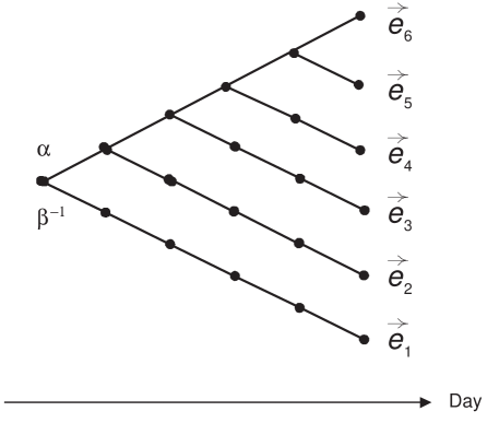
Fig. 2: The downturns.

Lemma 6.

1. Given a static algorithm ${\cal S}$, each $\vec{e}\in E$ is dominated by downturn $\vec{e}_{j}$, i.e., $\frac{{\cal A}(\vec{e})}{{\cal S}(\vec{e})}\leq\frac{{\cal A}(\vec{e}_{j})}{{\cal S}(\vec{e}_{j})}$, where $e_{j}=\max_{i=1}^{n}e_{i}$.

2. The smallest competitive ratio for the static algorithms is

   $${r_{\rm s}^{*}}=\inf_{f\in\Phi(Z_{n})}\max_{1\leq j\leq n}\frac{{\cal A}(\vec{e}_{j})}{\sum_{i=1}^{n}f(i)\,{\cal S}_{i}(\vec{e}_{j})}.$$

3. The static buy-and-hold trading problem can be regarded as a finite zero-sum two-person game $\Gamma_{K}(n,n)$ with the payoff matrix $K$ defined by $K(i,j)=\alpha^{i-j}$ if $i\leq j$ or $\beta^{j-i}$ if $i>j$, i.e.,

   $$K=\begin{array}[]{(}{ccccc})1&\alpha^{-1}&\alpha^{-2}&\cdots&\alpha^{1-n}\\ \beta^{-1}&1&\alpha^{-1}&\cdots&\alpha^{2-n}\\ \beta^{-2}&\beta^{-1}&1&\cdots&\alpha^{3-n}\\ \vdots&\vdots&\vdots&\ddots&\vdots\\ \beta^{1-n}&\beta^{2-n}&\beta^{3-n}&\cdots&1\end{array}.$$

Proof.

Statement 1 follows from the fact that $\frac{e_{j}}{e_{i}}\leq\alpha^{j-i}$ if $i\leq j$ and $\frac{e_{j}}{e_{i}}\leq\beta^{i-j}$ otherwise. Statement 2 follows from Equation (4) and Statement 1. For Statement 3, we let ${\cal S}_{i}$ be the online player’s $i$-th pure strategy; and let $\vec{e}_{j}$ be the the adversary’s $j$-th pure strategy. As in §2, the payoff matrix $K$ is defined by $K(i,j)=\frac{{\cal S}_{i}(\vec{e}_{j})}{{\cal A}(\vec{e}_{j})}$. The statement then follows from the facts that ${\cal A}(\vec{e}_{j})=\alpha^{j}$ and that ${\cal S}_{i}(\vec{e}_{j})=\alpha^{i}$ if $i\leq j$ or $\alpha^{j}\beta^{j-i}$ otherwise. ∎

In light of Lemma 6, an optimal mixed strategy of the online player of $\Gamma_{K}(n,n)$ corresponds to an optimal static algorithm. Thus, we next solve $\Gamma_{K}(n,n)$ to derive an optimal static algorithm.

3.3 Deriving an optimal static algorithm

Lemma 7.

For $n\geq 2$, $\det(K)=(1-\alpha^{-1}\beta^{-1})^{n-1}>0$.

Proof.

We use $K_{n}$ to emphasize the dimension $n$ of $K$. Let $A_{ij}$ be the submatrix of $K_{n}$ obtained by deleting row $i$ and column $j$. To expand $\det(K_{n})$ along the first row of $K_{n}$, observe that $A_{11}=K_{n-1}$. Furthermore, the first column of $A_{12}$ equals $\beta^{-1}$ times that of $A_{11}$, while the other columns of $A_{12}$ equal the corresponding ones of $A_{11}$; thus $\det(A_{12})=\beta^{-1}\det(A_{11})$. For $j=3,\ldots,n$, $\det(A_{1j})=0$ because in $A_{1j}$, the first column equals $\beta^{-1}$ times the second column. Hence, $\det(K_{n})=\det(A_{11})-\alpha^{-1}\det(A_{12})=\det(K_{n-1})-\alpha^{-1}\beta^{-1}\det(K_{n-1})=(1-\alpha^{-1}\beta^{-1})\det(K_{n-1}).$ The lemma immediately follows by induction on $n$. ∎

Let $b^{*}$ be the column vector of $n$ components defined by

$$b_{i}^{*}=\begin{cases}\frac{\alpha(\beta-1)}{n\alpha\beta-(n-1)(\alpha+\beta)+(n-2)}\quad\qquad i=1;\\ \frac{(\alpha-1)(\beta-1)}{n\alpha\beta-(n-1)(\alpha+\beta)+(n-2)}\quad\qquad 1<i<n;\\ \frac{(\alpha-1)\beta}{n\alpha\beta-(n-1)(\alpha+\beta)+(n-2)}\quad\qquad i=n.\end{cases}$$ (5)

Since ${b^{*}}>0$ and ${b^{*}}^{T}u_{n}=1$, $b^{*}$ represents a mixed strategy of the online player. So let ${\rm BAL}$ denote the static algorithm which applies ${\cal S}_{i}$ with probability $b_{i}^{*}$; note that by Lemma 5, ${\rm BAL}$ is equivalent to the deterministic static algorithm which invests $b_{i}^{*}$ dollars on the $i$-th day. Let ${c^{*}}$ be the vector obtained by swapping the first and $n$-th components of $b^{*}$. Similarly, ${c^{*}}>0$ and ${c^{*}}^{T}u_{n}=1$, and we intend ${c^{*}}$ to represent a mixed strategy of the adversary.

The next theorem analyzes ${\rm BAL}$. In light of Statement 3 of the theorem, we call ${\rm BAL}$ the balanced strategy.

Theorem 8.

Let $r=\frac{n\alpha\beta-(n-1)(\alpha+\beta)+(n-2)}{\alpha\beta-1}$.

1. ${\rm BAL}$ is an optimal static algorithm, and $\Upsilon_{\rm BAL}={r_{\rm s}^{*}}=r.$

2. ${\rm BAL}$ is the only optimal static algorithm subject to the equivalence stated in Lemma 5.

3. For $j=1,\ldots,n,\frac{{\cal A}(\vec{e}_{j})}{{\rm BAL}(\vec{e}_{j})}=\Upsilon_{\rm BAL}$; in other words, ${\rm BAL}$ has the same performance relative to the adversary’s on every downturn.

Proof.

Let $\bar{b}=rb^{*}$, and $\bar{c}=r{c^{*}}$. By Lemma 7, $K^{-1}$ exists. Below we prove $\bar{b}^{T}=u_{n}^{T}K^{-1}$ and $\bar{c}=K^{-1}u_{n}$. Then, Statement 1 follows from Theorem 4(2) and the fact that $\bar{b}\geq 0$, $\bar{c}\geq 0$, and $\bar{b}^{T}u_{n}=r$. Statement 2 follows from Theorem 4(4) and the fact that every component of $\bar{b}$ and $\bar{c}$ is greater than $0$. Statement 3 follows from Theorem 4(3)

To prove $\bar{b}^{T}=u_{n}^{T}K^{-1}$ and $\bar{c}=K^{-1}u_{n}$, observe that $\bar{c}$ can be obtained by swapping $\alpha$ and $\beta$ in $\bar{b}$, and the $j$-th column $K^{j}$ of $K$ can be obtained from the $j$-th row of $K$ by the same operation. Therefore, $\bar{b}^{T}K=u_{n}^{T}$ if and only if $K\bar{c}=u_{n}$, and we only need to establish $\bar{b}^{T}K=u_{n}^{T}$. Since $\bar{b}^{T}K^{1}=1$ if and only if $\bar{b}^{T}K^{n}=1$, we only show $\bar{b}^{T}K^{j}=1$ for $1\leq j<n$ as follows:

$$\bar{b}^{T}K^{j} =\sum_{i=1}^{n}\bar{b}_{i}K(i,j)$$

$$=\frac{1}{\alpha\beta-1}\left[\alpha(\beta-1)\alpha^{1-j}+\sum_{1<i\leq j}(\alpha-1)(\beta-1)\alpha^{i-j}+\right.$$

$$\,\qquad\qquad\left.\sum_{j<i<n}(\alpha-1)(\beta-1)\beta^{j-i}+(\alpha-1)\beta\beta^{j-n}\right]$$

$$=\frac{1}{\alpha\beta-1}\left[\alpha^{2-j}(\beta-1)+(\alpha-\alpha^{2-j})(\beta-1)+\right.$$

$$\,\qquad\qquad\left.(\alpha-1)(1-\beta^{j-n+1})+(\alpha-1)\beta^{j-n+1}\right]$$

$$=\frac{1}{\alpha\beta-1}\left(\alpha\beta-1\right)$$

$$=1.$$

∎

3.4 Comparison with the dollar averaging strategy

The dollar averaging strategy (${\rm DA}$) is the static algorithm which invests an equal amount of capital, i.e., $1/n$ dollars, on each trading day. Thus, by Lemma 5, ${\rm DA}$ is the uniformly mixed strategy for the online player in the game $\Gamma_{K}(n,n)$. By Theorem 8, ${\rm DA}$ is not an optimal static algorithm, and $\Upsilon_{\rm BAL}<\Upsilon_{\rm DA}$. The next lemma gives a closed-form formula of $\Upsilon_{\rm DA}$. Figure 3 plots the relationship between $\Upsilon_{{\rm DA}}$ and $\Upsilon_{{\rm BAL}}$ for $2\leq n\leq 100$.

Lemma 9.

$\Upsilon_{\rm DA}=\max\left\{\frac{n(1-\alpha^{-1})}{1-\alpha^{-n}},\frac{n(1-\beta^{-1})}{1-\beta^{-n}}\right\}.$

Proof.

Let $B_{j}=\sum_{i=1}^{n}K(i,j)$. By Lemma 6, $\Upsilon_{{\rm DA}}=\max_{1\leq j\leq n}\frac{n}{B_{j}}$. By algebra, $B_{j+1}-B_{j}$ is a decreasing function of $j$. Thus, $B_{j}$ is a function of $j$ whose minimum occurs at one end of the domain $\{1,\ldots,n\}$. The lemma follows from this concavity. ∎

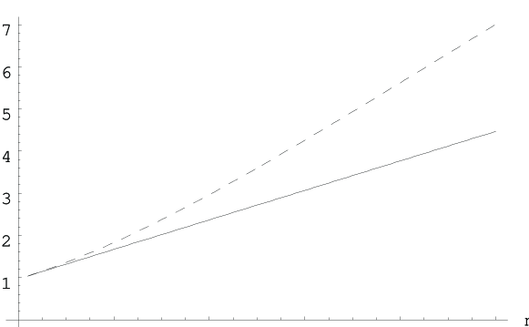
Fig. 3: The dashed and solid dotted lines denote $\Upsilon_{{\rm DA}}$ and $\Upsilon_{{\rm BAL}}$, respectively, with $\alpha=1/0.93$ and $\beta=1.07$.

We have also experimented with ${\rm BAL}$ and ${\rm DA}$ using Taiwan’s market data. As shown in Figure 1, the Taipei Stock Exchange (TSE) adopts $\alpha=1/0.93$ and $\beta=1.07$. We select the Taiwan Semiconductor Manufacturing Company (TSMC) and Acer Computer Company (Acer) for experimental analysis. TSMC is the largest foundry of wafer manufacturing in the world and is listed on both TSE and the New York Stock Exchange (NYSE) under the symbol TSM. Acer is the world’s third largest PC manufacturer as well as the fifth largest mobile PC manufacturer.

Figure 4 shows the daily closing prices of TSMC in 1997. All stock prices are quoted in the New Taiwan dollar (NT dollar). One investment plan is executed each month. Each plan buys shares of TSMC with an initial capital of one NT dollar as in §3; however, the exchange rate of a day is the reciprocal of that day’s share price without an initial normalization to one. A monthly accumulation is the total number of shares acquired over a month. For ease of comparison, a monthly accumulation is expressed in NT dollar by converting the acquired shares into NT dollars at the price of the last trading day of each month. Figure 5 shows the monthly accumulations of ${\rm BAL}$ and ${\rm DA}$ on TSMC for each month of 1997. Notice that ${\rm BAL}$ and ${\rm DA}$ are money-making except in September, October, and December. Figure 6 shows the realized competitive ratios of ${\rm BAL}$ and ${\rm DA}$, which are the performance ratios as defined in Equation (1) but with $\vec{e}$ set to the actual exchange rate sequences. Note that for all twelve months, these ratios are less than $1.35$. For visual clarity, we join the monthly accumulations and competitive ratios by line segments, and use the solid and dotted lines to denote the graphs of ${\rm BAL}$ and ${\rm DA}$, respectively. Observe that overall, ${\rm BAL}$ outperforms ${\rm DA}$.

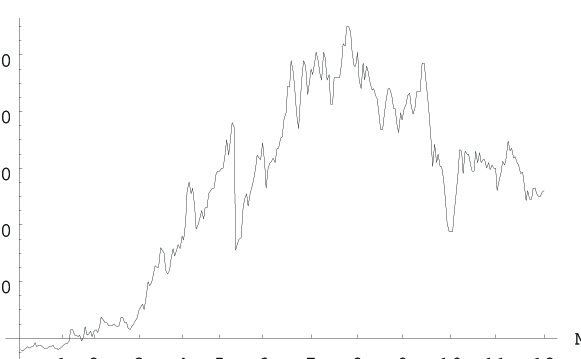
Fig. 4: TSMC’s daily closing stock prices in 1997.

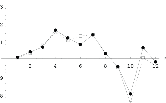
Fig. 5: Accumulations of ${\rm BAL}$ and ${\rm DA}$ on TSMC.

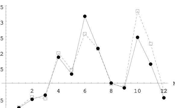
Fig. 6: Realized competitive ratios of ${\rm BAL}$ and ${\rm DA}$ on TSMC.

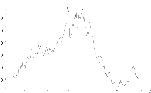
Fig. 7: Acer’s daily closing stock prices in 1997.

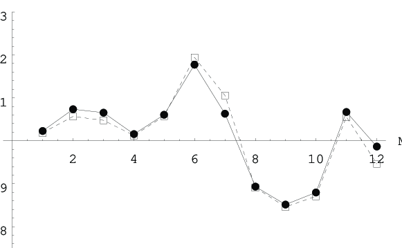
Fig. 8: Accumulations of ${\rm BAL}$ and ${\rm DA}$ on Acer.

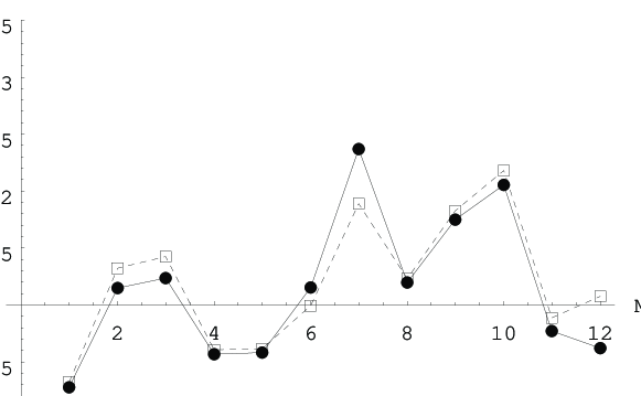
Fig. 9: Realized competitive ratios of ${\rm BAL}$ and ${\rm DA}$ on Acer.

Figure 7 shows the daily closing prices of Acer in 1997. Figures 8 and 9 show the monthly accumulations and realized competitive ratios of ${\rm BAL}$ and ${\rm DA}$, respectively. The experimental results for Acer lead to similar conclusions to those for TSMC.

4 Open problems

We have presented the balanced strategy ${\rm BAL}$ and proved its unique optimality among the static algorithms. Furthermore, each of its exact competitive ratio and daily investment amounts has a closed-form expression which takes $O(1)$ time to evaluate. In light of these results, an immediate open problem is whether there are similar results for dynamic online trading algorithms. There are two orthogonal directions for further research as follows.

One direction is to change the assumption that the time horizon is fixed and known a priori to ${\cal B}$. For instance, it would be meaningful to consider the scenario that there is a cash stream instead of a one-time capital at the beginning of the investment horizon. For this scenario, an investor might need to guess when the cash stream will end.

The other direction is to replace $\alpha$ and $\beta$ with a known probability distribution of the ratio $\frac{e^{\prime}}{e}$. This would be an example of the standard approach in finance of considering the average-case performance under an assumed probabilistic model. While the worst-case approach in computer science is unnecessarily pessimistic, the average-case approach in finance is overly dependent on the chosen model. In general. it would be of interest to combine these two approaches to formulate more informative computational problems than either approach could.

References

- [1] M. Ajtai, N. Megiddo, and O. Waarts, Improved algorithms and analysis for secretary problems and generalizations, in Proceedings of the 36th Annual Symposium on Foundations of Computer Science, 1995, pp. 473–482.
- [2] S. al-Binali, The competitive analysis of risk taking with application to online trading, in Proceedings of the 38th Annual IEEE Symposium on Foundations of Computer Science, 1997, pp. 336–344.
- [3] M. Baxter and A. Rennie, Financial Calculus: an Introduction to Derivative Pricing, Cambridge University Press, Cambridge, United Kingdom, 1996.
- [4] A. Borodin and R. El-Yaniv, Online Computation and Competitive Analysis, Cambridge University Press, Cambridge, United Kingdom, 1998.
- [5] A. Chou, J. Cooperstock, R. El-Yaniv, M. Klugerman, and T. Leighton, The statistical adversary allows optimal money-making trading strategies, in Proceedings of the 6th Annual ACM-SIAM Symposium on Discrete Algorithms, 1995, pp. 467–476.
- [6] Y. S. Chow, S. Moriguti, H. Robbins, and S. M. Samuels, Optimal selection based on relative rank the secretary problem, Israel Journal of Mathematics, 2 (1964), pp. 81–90.
- [7] T. Cover and E. Ordentlich, Universal portfolios with side information, IEEE Transactions on Information Theory, 42 (1996).
- [8] T. M. Cover, Universal portfolio, Mathematical Finance, 1 (1991), pp. 1–29.
- [9] D. Duffie, Dynamic Asset Pricing Theory, Princeton University Press, Princeton, NJ, 1996.
- [10] R. El-Yaniv, Competitive solutions for online financial problems, ACM Computing Surveys, 30 (1998), pp. 28–69.
- [11] R. El-Yaniv, A. Fiat, R. M. Karp, and G. Turpin, Competitive analysis of financial games, in Proceedings of the 33rd Annual IEEE Symposium on Foundations of Computer Science, 1992, pp. 327–333.
- [12] , Optimal search and one-way trading online algorithms. Manuscript, 1997.
- [13] P. Freeman, The secretary problem and its extensions, International Statistical Review, 51 (1983), pp. 189–206.
- [14] J. Hull, Options, Futures, and Other Derivatives, Prentice-Hall, Upper Saddle River, NJ, 3rd ed., 1997.
- [15] M. Y. Kao and S. R. Tate, Online matching with blocked input, Information Processing Letters, 38 (1991), pp. 113–116.
- [16] , On-line difference maximization, in Proceedings of the 8th Annual ACM-SIAM Symposium on Discrete Algorithms, 1997, pp. 175–182.
- [17] R. M. Karp, U. V. Vazirani, and V. V. Vazirani, An optimal algorithm for on-line bipartite matching, in Proceedings of the 22nd Annual ACM Symposium on Theory of Computing, 1990, pp. 352–358.
- [18] Y. D. Lyuu, Financial Engineering and Computation: Principles, Mathematics, Algorithms, To be published, 1999.
- [19] K. R. MacCrimmon and D. A. Wehrung, Taking Risks: The Management of Uncertainty, Free Press, New York, NY, 1986.
- [20] S. N. Neftci, An Introduction to the Mathematics of Financial Derivatives, Academic Press, New York, NY, 1996.
- [21] E. Ordentlich and T. Cover, On-line portfolio selection, in Proceedings of the 9th Conference on Computational Learning Theory, 1996, pp. 310–313.
- [22] L. A. Petrosjan and N. A. Zenkevich, Game Theory, World Scientific, Singapore, 1996.
- [23] T. Raghavan, Zero-sum two-person games, in Handbook of Game Theory, R. Aumann and S. Hart, eds., vol. 2, Elsevier Science Publishers B. V., 1994, pp. 735–759.
- [24] W. F. Sharpe, G. J. Alexander, and J. V. Bailey, Investments, Prentice-Hall, Upper Saddle River, NJ, 5th ed., 1995.
- [25] D. Sleator and R. E. Tarjan, Amortized efficiency of list update and paging rules, Communications of the ACM, 28 (1985), pp. 202–208.
- [26] P. Wilmott, S. Howison, and J. Dewynne, The Mathematics of Financial Derivatives, Cambridge University Press, Cambridge, United Kingdom, 1995.
- [27] A. C. C. Yao, New algorithms for bin packing, Journal of the ACM, 27 (1980), pp. 207–227.