Designing Proxies for Stock Market Indices
is Computationally Hard

Abstract

In this paper, we study the problem of designing proxies (or portfolios) for various stock market indices based on historical data. We use four different methods for computing market indices, all of which are formulas used in actual stock market analysis. For each index, we consider three criteria for designing the proxy: the proxy must either track the market index, outperform the market index, or perform within a margin of error of the index while maintaining a low volatility. In eleven of the twelve cases (all combinations of four indices with three criteria except the problem of sacrificing return for less volatility using the price-relative index) we show that the problem is NP-hard, and hence most likely intractable.

1 Introduction

Market indices are widely used to track the performance of stocks or to design investment portfolios [1]. This paper initiates a rigorous mathematical study of the computational complexity of the art of designing proxies for such indices. There are several results on selecting such proxies (or portfolios) in an on-line manner (see, for example, [2] and [3]), but we look at off-line algorithms for designing proxies based on historical data. In particular, we show that, with one exception, all combinations of three fundamental problems (such as tracking or outperforming a full market index) with four commonly-used indices give NP-complete problems, so are computationally hard. We conjecture that the one remaining problem is also NP-complete, but do not have a proof at this time.

To formally define market indices, let ${\cal B}$ be a set of $b$ stocks in a market. Let $S_{i,t}\geq 0$ be the price of the $i$-th stock at time $t$. Let $w_{i}$ be the number of outstanding shares of the $i$-th stock. We assume that $w_{i}$ does not change with time. This paper discusses computational complexity issues regarding four kinds of market indices currently in use [1]. These indices are calculated by the following formulas, which can be multiplied by arbitrary constants to arrive at desired starting index values at time 0.

$\bullet$ The price-weighted index of ${\cal B}$ at time $t$ is

$$\Phi_{1}({\cal B},t)=\frac{\sum_{i=1}^{b}{S_{i,t}}}{b}.$$ (1)

The Dow Jones Industrial Average is calculated in this manner for some ${\cal B}$ consisting of thirty stocks.

$\bullet$ The value-weighted index of ${\cal B}$ at time $t$ is

$$\Phi_{2}({\cal B},t)=\frac{\sum_{i=1}^{b}{w_{i}{\cdot}S_{i,t}}}{\sum_{i=1}^{b}{w_{i}{\cdot}S_{i,0}}}.$$

The Standard & Poor’s 500 is computed in this way with respect to 500 stocks.

$\bullet$ The equal-weighted index of ${\cal B}$ at time $t$ is

$$\Phi_{3}({\cal B},t)=\sum_{i=1}^{b}\frac{S_{i,t}}{S_{i,0}}.$$

The index published by the Indicator Digest is calculated by this method, involving stocks listed on the New York Stock Exchange.

$\bullet$ The price-relative index of ${\cal B}$ at time $t$ is

$$\Phi_{4}({\cal B},t)=\left(\Pi_{i=1}^{b}\frac{S_{i,t}}{S_{i,0}}\right)^{\frac{1}{b}}.$$

The Value Line Index is computed by this formula.

There are numerous reasons why stock investors and money managers would want to invest in a subset of stocks rather than those of a whole market [1]. For instance, small investors certainly do not have sufficient capital to invest in every stock in the market. Logically, such investors would attempt to choose a small subset of stocks which hopefully can perform roughly as well as or even outperform the market as a whole. They then face difficult trade-offs between returns and risks. For these and other reasons of optimization, we formulate three natural computational problems for the design of market indices. Given a market ${\cal M}$ consisting of $m$ stocks, we wish to choose a subset ${\cal M}_{k}$ of at most $k$ stocks and calculate an index of ${\cal M}_{k}$, which is called a $k$-proxy of the corresponding index of the whole market ${\cal M}$ (we sometimes refer to ${\cal M}_{k}$ as a portfolio). Our goal is to choose ${\cal M}_{k}$ so that the resulting $k$-proxy tracks or outperforms the corresponding index of ${\cal M}$. This paper shows that designing proxies for the above four indices based on historical data is computationally hard.

We note here that while our problem statements might sound rather restrictive since error bounds must be met for every time step, we can use simple padding arguments to extend all of our proofs to more relaxed problems of the form “can the error bound be met $x$ percent of the time?”

2 Problem Formulations

In this section we formally define three basic problems related to selecting $k$-proxies, or portfolios.

Problem 1 (tracking an index)

• Input: A market ${\cal M}$ of $m$ stocks, their prices $S_{i,t}\geq 0$ for $t=0,\ldots,f$, their numbers $w_{i}$ of outstanding shares, a real $\epsilon_{1}>0$, an integer $k>0$, and some $j\in\{1,2,3,4\}$ to indicate the desired type of index.

• Output: A subset ${\cal M}_{k}$ of at most $k$ stocks in ${\cal M}$ such that

  $$\left|\frac{\Phi_{j}({\cal M}_{k},t)}{\Phi_{j}({\cal M}_{k},0)}-\frac{\Phi_{j}({\cal M},t)}{\Phi_{j}({\cal M},0)}\right|\leq\epsilon_{1}{\cdot}\frac{\Phi_{j}({\cal M},t)}{\Phi_{j}({\cal M},0)}\mbox{ for all }t=1,\ldots,f.$$ (2)

Problem 2 (outperforming an index)

• Input: A market ${\cal M}$ of $m$ stocks, their prices $S_{i,t}\geq 0$ for $t=0,\ldots,f$, their numbers $w_{i}$ of outstanding shares, a real $\epsilon_{2}\geq 0$, an integer $k>0$, and some $j\in\{1,2,3,4\}$ to indicate the desired type of index.

• Output: A subset ${\cal M}_{k}$ of at most $k$ stocks in ${\cal M}$ such that

  $$\frac{\Phi_{j}({\cal M}_{k},t)}{\Phi_{j}({\cal M}_{k},0)}\geq(1+\epsilon_{2}){\cdot}\frac{\Phi_{j}({\cal M},t)}{\Phi_{j}({\cal M},0)}\mbox{ for all }t=1,\ldots,f.$$ (3)

For the final problem, we need a few extra definitions in order to analyze the volatility of a set of stocks. Let ${\cal B}$ be a set of stocks as defined in §1.

$\bullet$ The one-period return of $\Phi_{j}$ for ${\cal B}$ at time $t\geq 1$ is

$$R_{j}({\cal B},t)=\ln\frac{\Phi_{j}({\cal B},t)}{\Phi_{j}({\cal B},t-1)}.$$

$\bullet$ The average return of $\Phi_{j}$ for ${\cal B}$ up to time $t\geq 1$ is

$$\overline{R}_{j}({\cal B},t)=\frac{\sum_{i=1}^{t}R_{j}({\cal B},i)}{t}.$$

$\bullet$ The volatility of $\Phi_{j}$ for ${\cal B}$ up to time $t\geq 2$ is

$$\Delta_{j}({\cal B},t)=\sqrt{\frac{\sum_{i=1}^{t}\left(R_{j}({\cal B},i)-\overline{R}_{j}({\cal B},t)\right)^{2}}{t-1}}.$$

Problem 3 (sacrificing return for less volatility)

• Input: A market ${\cal M}$ of $m$ stocks, their prices $S_{i,t}\geq 0$ for $t=0,\ldots,f$, their numbers $w_{i}$ of outstanding shares, two reals $\alpha,\beta>0$, an integer $k>0$, and some $j\in\{1,2,3,4\}$ to indicate the desired type of index.

• Output: A subset ${\cal M}_{k}$ of at most $k$ stocks in ${\cal M}$ such that

  $$\frac{\Phi_{j}({\cal M}_{k},t)}{\Phi_{j}({\cal M}_{k},0)}\geq\alpha{\cdot}\frac{\Phi_{j}({\cal M},t)}{\Phi_{j}({\cal M},0)}\mbox{ for all }t=1,\ldots,f;$$ (4)

  $$\Delta_{j}({\cal M}_{k},s)\leq\beta{\cdot}\Delta_{j}({\cal M},s)\mbox{ for all }s=2,\ldots,f.$$ (5)

  In this problem, (4) is called the performance bound, and (5) is called the volatility bound.

3 Price-weighted Index

In this section, we consider taking the value of the market and portfolio using a price-weighted index, defined in (1). As given in the problem statements, we use the notation $\Phi_{1}({\cal M},t)$ to denote the market average at timestep $t$, and $\Phi_{1}({\cal M}_{k},t)$ to denote the average of the portfolio at that timestep.

3.1 Tracking an index

To solve the problem of tracking the market average, we need to satisfy (2) using function $\Phi_{1}({\cal B},t)$. We will refer to this bound as the “tracking bound.” In the following proofs, we show this by proving an equivalent relation:

$$1-\epsilon\leq\frac{\Phi_{1}({\cal M},0)}{\Phi_{1}({\cal M}_{k},0)}\cdot\frac{\Phi_{1}({\cal M}_{k},t)}{\Phi_{1}({\cal M},t)}\leq 1+\epsilon.$$ (6)

Theorem 3.1

Let $\epsilon$ be any error bound satisfying $0<\epsilon<1$ and specified using $n^{O(1)}$ bits in fixed point notation. Then the tracking problem for a price-weighted index with error bound $\epsilon$ is NP-hard.

In the remainder of this section, we prove this theorem by reduction from the minimum set cover problem. We will use the notation from the minimum cover definition given in the classic book on NP-completeness by Garey and Johnson [4]: $C$ is a collection of subsets of a finite set $S$, and $K$ is the desired cover size. Specifically, we want a subcollection $C^{\prime}\subseteq C$ such that $|C^{\prime}|\leq K$ and every item $x\in S$ is in some subset from $C^{\prime}$.

Let $n=|C|$, and consider making an $n\times|S|$ matrix in which each column corresponds to a fixed item from $S$, and each row corresponds to a subset $S^{\prime}\in C$. The element in row $i$, column $j$ is some given value $v_{1}$ if the element in $S$ for that column is in the subset $S^{\prime}$, and value $v_{0}$ if it is not. Then the minimum cover problem can be stated as follows: Is there a set of $K$ rows such that the $K\times|S|$ matrix defined using only those rows has at least one entry with value $v_{1}$ in each column?

It makes sense now to consider this $n\times|S|$ matrix as an input to the portfolio selection problem, where each row corresponds to a stock and each column corresponds to a timestep, and we are to choose a portfolio of size $k=K$. Selecting a portfolio is then equivalent to selecting the subcollection in the minimum cover problem. A subcollection that is missing some item from $S$ corresponds to a portfolio in which some timestep has all values equal to $v_{0}$, and hence the portfolio average at that timestep must be $v_{0}$. Ideally, we would select $v_{0}$ and $v_{1}$ in such a way that the required tracking bound is met if any $v_{1}$ values are included in the portfolio, but not if all values are $v_{0}$. However, this simple construction has very unpredictable market averages at each time step, so we need a slightly more involved construction.

We will introduce a new row into our matrix called the “adjustment row”, and we will select values to adjust the column averages to predictable values. To guarantee that this row is not selected in our portfolio (so selections are made up entirely of rows from the minimum cover problem), we introduce a special column called the “control column” — any selection including our adjustment row will violate the error bound in that column, and no selection excluding that row will violate the bound. In addition, we need to pad the problem out substantially. This is accomplished by including rows that contain value $v_{0}$ in every non-control column, which is equivalent to padding the original set cover problem instance with empty subsets added to $C$. This clearly has no effect on the set cover problem. Finally, we insert a column of all ones to give the $S_{i,0}$ values for the portfolio selection problem. The final matrix contains $m=3n$ rows, $f=|S|+2$ columns, and is depicted in Figure 1.

Note that since $S_{i,0}=1$ for all $i$, $\Phi_{1}({\cal M},0)=\Phi_{1}({\cal M}_{k},0)=1$, and so (6) reduces to just checking that

$$1-\epsilon\leq\frac{\Phi_{1}({\cal M}_{k},t)}{\Phi_{1}({\cal M},t)}\leq 1+\epsilon.$$

Figure 1: Pictorial depiction of reduction for Theorem 3.1

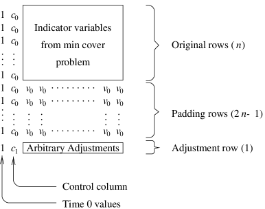
First we examine properties of the control column, where the values in that column are defined by

$$c_{0} = \left\lceil\frac{1-\epsilon}{\epsilon}\right\rceil,$$

$$c_{1} = c_{0}+m.$$

Lemma 3.1

The tracking bound is met for the control column if and only if the adjustment row is not included in the portfolio.

Proof: From the values for $c_{0}$ and $c_{1}$, it is clear that the average value of the control column is $c_{0}+1$. Since we will be examining the error of approximations relative to this average, we first note that we can bound (due to the ceiling involved in the definition of $c_{0}$)

$$\frac{\epsilon}{1+\epsilon}<\frac{1}{c_{0}+1}\leq\epsilon.$$ (7)

Any portfolio that does not include the adjustment row has average value $c_{0}$, and so we can lower bound the relative error by

$$\frac{\Phi_{1}({\cal M}_{k},t)}{\Phi_{1}({\cal M},t)}=\frac{c_{0}}{c_{0}+1}=1-\frac{1}{c_{0}+1}\geq 1-\epsilon.$$

Since the relative error is clearly less than one, it falls into the acceptable range of values.

On the other hand, if a portfolio does include the adjustment row, then the portfolio average is $c_{0}+m/k$, and so the relative error is

$$\frac{\Phi_{1}({\cal M}_{k},t)}{\Phi_{1}({\cal M},t)}=\frac{c_{0}+m/k}{c_{0}+1}=1+\frac{m/k-1}{c_{0}+1}.$$

Due to our padding of the problem, we know that $k\leq m/3$, and so $m/k-1\geq 2$. Using this observation and the bound from (7) leads to the conclusion that

$$\frac{\Phi_{1}({\cal M}_{k},t)}{\Phi_{1}({\cal M},t)}\geq 1+\frac{2}{c_{0}+1}>1+\frac{2}{1+\epsilon}\,\epsilon>1+\epsilon.$$

In other words, any portfolio that includes the adjustment row will not meet the required error bound. Combined with our previous observation, this completes the proof of the lemma.     

Next we must define the values $v_{0}$ and $v_{1}$, and show the equivalence of our portfolio selection instance with the original set cover instance. To do so, define

$$v_{0} = \left\lceil k\frac{1-\epsilon}{\epsilon}\right\rceil,$$

$$\Delta = k+\left\lceil\frac{\epsilon}{1-\epsilon}\right\rceil,$$

$$v_{1} = v_{0}+\Delta.$$

Note that since $\epsilon<1$, all these values are clearly non-negative integers, as required by the portfolio selection problem.

For column $t$, if there are $M_{t}$ rows with value $v_{1}$, then the value we use in the adjustment row for that column is

$$A_{t}=v_{0}+(m-M_{t})\Delta\ ,$$

which is clearly a positive integer, since $M_{t}<m$. The sum down the column is

$$(m-M_{t}-1)v_{0}+M_{t}v_{1}+A_{t} = (m-M_{t}-1)v_{0}+M_{t}(v_{0}+\Delta)+v_{0}+(m-M_{t})\Delta$$

$$= mv_{0}+m\Delta,$$

which means that the column average is $v_{0}+\Delta$, or just $v_{1}$. Notice the independence from $t$. We make such an adjustment for every column in the matrix.

We next demonstrate the equivalence of the produced portfolio selection instance with the original set cover instance.

Lemma 3.2

The relative error bound is met if and only if the portfolio contains at least one $v_{1}$ value in each column (other than the control column).

Proof: First, for the “only if” part of the lemma, consider the case where the relative error bound is met. Consider any specific column $t$ of our table, and assume that this column does not contain any $v_{1}$ values. By the last lemma, the adjustment row cannot be included in our portfolio, so all values must be $v_{0}$, and so the portfolio average is exactly $v_{0}$. Therefore, we can derive

$$\frac{\Phi_{1}({\cal M}_{k},t)}{\Phi_{1}({\cal M},t)}=\frac{v_{0}}{v_{0}+\Delta}=\frac{1}{1+\frac{\Delta}{v_{0}}},$$ (8)

and so providing a good lower bound for $\frac{\Delta}{v_{0}}$ would in fact upper bound this ratio. We can do this as follows:

$$\frac{\Delta}{v_{0}}=\frac{k+\left\lceil\frac{\epsilon}{1-\epsilon}\right\rceil}{\left\lceil k\frac{1-\epsilon}{\epsilon}\right\rceil}>\frac{k+\frac{\epsilon}{1-\epsilon}}{k\frac{1-\epsilon}{\epsilon}+1}=\frac{\frac{k(1-\epsilon)+\epsilon}{1-\epsilon}}{\frac{k(1-\epsilon)+\epsilon}{\epsilon}}=\frac{\epsilon}{1-\epsilon}.$$

Plugging back in to (8), we get

$$\frac{\Phi_{1}({\cal M}_{k},t)}{\Phi_{1}({\cal M},t)}<\frac{1}{1+\frac{\epsilon}{1-\epsilon}}=1-\epsilon.$$

Thus under our assumption that no $v_{1}$ values are included, the error bound is not met. We conclude that if the error bound is met, then at least one $v_{1}$ value must be included in each column.

Next, for the “if” part of the theorem, assume that each column in the selected portfolio contains at least one $v_{1}$ value and that we have not selected the adjustment row. Since the market average is $v_{1}$, and the largest possible selected value in the portfolio is $v_{1}$, we know that $\Phi_{1}({\cal M}_{k},t)\leq\Phi_{1}({\cal M},t)$, and so the upper bound $1+\epsilon$ on the relative error is trivially met for any $\epsilon\geq 0$.

Since we have selected at least one $v_{1}$ value, the portfolio average is at least $v_{0}+\Delta/k$, and so to lower bound the relative error notice that

$$\frac{\Phi_{1}({\cal M}_{k},t)}{\Phi_{1}({\cal M},t)}\geq\frac{v_{0}+\frac{\Delta}{k}}{v_{0}+\Delta}=1-\frac{k-1}{k}\cdot\frac{1}{\frac{v_{0}}{\Delta}+1}.$$ (9)

Now we will derive a lower bound for $\frac{v_{0}}{\Delta}$ in a similar way to what we did above, so

$$\frac{v_{0}}{\Delta}=\frac{\left\lceil k\frac{1-\epsilon}{\epsilon}\right\rceil}{k+\left\lceil\frac{\epsilon}{1-\epsilon}\right\rceil}>\frac{k\frac{1-\epsilon}{\epsilon}}{k+\frac{\epsilon}{1-\epsilon}+1}=\frac{\frac{k(1-\epsilon)}{\epsilon}}{\frac{k(1-\epsilon)+1}{1-\epsilon}}=\frac{1-\epsilon}{\epsilon}\cdot\frac{k(1-\epsilon)}{k(1-\epsilon)+1}.$$

Using this bound, with a little manipulation we can derive

$$\frac{k-1}{k}\cdot\frac{1}{\frac{v_{0}}{\Delta}+1}<\frac{k-1}{k}\cdot\frac{(1-\epsilon)k+1}{(1-\epsilon)k+\epsilon}\cdot\epsilon.$$

We can bound the middle factor of this bound by $\frac{k+1}{k}$ by noticing that

$$\frac{(1-\epsilon)k+1}{(1-\epsilon)k+\epsilon}<\frac{k+1}{k}\mbox{\hskip 14.45377pt$\Longleftarrow$\hskip 14.45377pt}(1-\epsilon)k^{2}+k<(1-\epsilon)k^{2}+\epsilon k+(1-\epsilon)k+\epsilon\mbox{\hskip 14.45377pt$\Longleftarrow$\hskip 14.45377pt}0<\epsilon,$$

and so plugging back into (9) we get

$$\frac{\Phi_{1}({\cal M}_{k},t)}{\Phi_{1}({\cal M},t)}\geq 1-\frac{1}{\frac{v_{0}}{\Delta}+1}>1-\frac{k-1}{k}\cdot\frac{k+1}{k}\cdot\epsilon=1-\frac{k^{2}-1}{k^{2}}\cdot\epsilon>1-\epsilon.$$

We conclude that if at least one value in column $t$ of the selected portfolio is $v_{1}$, then the relative error bound is met. Since we have completed both directions of the “if and only if” proof, this completes the proof of the lemma.     

As a final note, it is fairly easy to show that all values in the constructed portfolio selection problem have length polynomial in the length of the original set cover problem and the number of bits used to specify $\epsilon$. Therefore, these values form a polynomial time reduction from the set cover problem to the portfolio selection problem, which completes the proof of Theorem 3.1.

3.2 Sacrificing Return for Less Volatility

Next, we will skip Problem 2 and prove a hardness result for Problem 3: sacrificing return for less volatility. In the following section, we will return to problem 2, and show that the hardness of that problem (outperforming an index) follows directly from the results of this section.

As in §3.1, we will show that Problem 3 is NP-complete by reducing the minimum cover problem to this one.

3.2.1 The construction

Figure 2: Construction for main reduction of Section 3.2

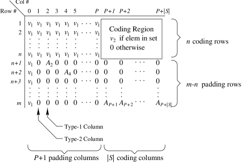
The main reduction for this proof involves a problem constructed from a minimum cover instance, and this construction is illustrated in Figure 2. This constructed problem is an instance of our portfolio selection problem where the rows represent different stocks, the columns represent times, and the values in the matrix represent prices.

In the original minimum cover instance, let $n=|C|$ represent the number of subsets in the input, let $|S|$ represent the size of the overall set, and let $K$ be the number of subsets we are allowed to select. The data from this problem can be encoded into an $n\times|S|$ matrix $M$, where the values in this matrix are set as follows ($v_{2}$ is a value that will be defined shortly):

$$M_{ij}=\left\{\begin{array}[]{ll}v_{2}&\mbox{ if subset $i$ contains element $j$;}\\ 0&\mbox{ otherwise.}\end{array}\right.$$

We will need a larger matrix in order to complete the reduction, so we embed matrix $M$ into our larger matrix — in Figure 2 the embedded matrix is labeled as the “Coding Region”. This gives a portfolio selection problem with $m$ stocks, $f=P+|S|$ time steps, and portfolio size $k=K$.

We surround matrix $M$ with various “padding rows” and “padding columns”. The number of padding rows and padding columns are defined as follows:

• There are $P+1$ padding columns, where $P=\max\left(2(k+1),2|S|\right)$.

• The total number of rows is defined in terms of the following constants:

  $$q=\left\lceil\max\left(1+(4/\beta),\log_{k}(2/\alpha)\right)\right\rceil,\hbox to72.26999pt{\hss and\hss}B=\left\lceil\alpha k^{q}\right\rceil.$$

  The total number of rows is $m=nB$.

The definition of $q$ implies some important properties of the constant $B$ that we note here:

$$B\geq 2;$$ (10)

$$B\geq k\alpha\geq\alpha.$$ (11)

Finally, from the first part of (11) we can derive

$$\left\lfloor\frac{B}{\alpha}\right\rfloor>\frac{B}{\alpha}\,\frac{k-1}{k}.$$ (12)

All of the first $n$ rows in the padding columns are filled with value $v_{1}$, and value $v_{2}$ is used in the coding region as previously described. These values are defined in terms of the constant $B$ as follows:

• $v_{1}=B-1$

• $v_{2}=k(B-1)$

Each column may have an “adjustment value”, denoted by $A_{t}$ for column $t$. Odd numbered columns in the padding region (type-2 columns) do not have an adjustment value, but even numbered columns other than column 0 (type-1 columns) do, and these values are positioned at successively lower rows; therefore, if column $t$ is a type-1 column, then $A_{t}$ is placed in row $n+\frac{t}{2}$. If we run out of rows before completing this placement, simply put all remaining adjustment values on the last row. Notice that since $P\geq 2(k+1)$ there are at least $k+1$ type-1 padding columns, and since the number of padding rows is $(m-n)=(nB-n)\geq n\geq k+1$ (using (10)), there must be at least $k+1$ distinct rows that contain adjustment values. Columns that cross the coding region (called “coding columns”) also have adjustment values, which are all placed on the last row of the matrix (see Figure 2). The adjustment values to be used are defined below, where $z_{t}$ is the number of zeros in the coding region of column $t$:

$$A_{t}=\left\{\begin{array}[]{ll}(m-n)\left(\left\lfloor\frac{B}{\alpha}\right\rfloor-1\right)&\mbox{ if $0<t\leq P$ and $t$ is even;}\\ \\ (m-n)\left(\left\lfloor\frac{B}{\alpha}\right\rfloor-k\right)+z_{t}\cdot v_{2}&\mbox{ if $t>P$.}\end{array}\right.$$

Note that the adjustment values in the padding columns are all the same, but the adjustments in the coding region depend on the data in the coding region. Furthermore, (11) guarantees that these adjustment values are all non-negative.

Before analyzing the return and volatility of the constructed portfolio selection problem, we state the following lemma regarding the size of the constructed problem, showing that we have a polynomial reduction — the proof of this lemma is straight-forward given the above definitions, and is omitted.

Lemma 3.3

If $\alpha$ and $\beta$ are expressed using $n^{O(1)}$ bits in fixed-point binary notation, and $0<\alpha\leq n^{O(1)}$ and $\beta=\Omega\left(\frac{\log k}{\log n}\right)$, then the size of the constructed problem (including the size of the values in the matrix) is polynomial in the size of the original minimum cover problem.

3.2.2 Guarantees on Return

Lemma 3.4

The performance bound is met for all columns if and only if the selected portfolio contains exactly $k$ items from the coding rows and each coding column has at least one $v_{2}$ value from among the selected rows.

Proof: We will first prove that if the selected portfolio contains exactly $k$ items from the coding rows and each coding column has at least one $v_{2}$ value from the selected rows, then the performance bound is met. First consider a padding column $t$ — since the $k$ selected rows are all coding rows, all selected values for any padding column have value $v_{1}$, and so the portfolio average for that column is $\Phi_{1}({\cal M}_{k},t)=v_{1}$. On the other hand, the market average is different for the two types of columns. If column $t$ is a type-1 padding column, then the sum of all the values in the column is

$$nv_{1}+A_{t} = n(B-1)+(m-n)\left(\left\lfloor\frac{B}{\alpha}\right\rfloor-1\right)=n(B-1)+(nB-n)\left(\left\lfloor\frac{B}{\alpha}\right\rfloor-1\right)$$

$$= n(B-1)+(B-1)\left(n\left\lfloor\frac{B}{\alpha}\right\rfloor-n\right)=(B-1)n\left\lfloor\frac{B}{\alpha}\right\rfloor.$$

Therefore, the market average for column $t$ satisfies

$$\Phi_{1}({\cal M},t) = \frac{(B-1)n}{nB}\left\lfloor\frac{B}{\alpha}\right\rfloor=\frac{B-1}{B}\,\left\lfloor\frac{B}{\alpha}\right\rfloor$$

$$\leq \frac{B-1}{B}\,\frac{B}{\alpha}=\frac{B-1}{\alpha}=\frac{v_{1}}{\alpha}.$$

Furthermore, any type-2 padding column has no adjustment value, which makes the market average smaller than a type-1 column. Therefore, for either type of padding column the bound $\Phi_{1}({\cal M},t)\leq\frac{v_{1}}{\alpha}$ is valid, and so it immediately follows that for any padding column $t$, since $\Phi_{1}({\cal M},0)=\Phi_{1}({\cal M}_{k},0)=v_{1}$,

$$\frac{\Phi_{1}({\cal M}_{k},t)}{\Phi_{1}({\cal M}_{k},0)}\geq\alpha\cdot\frac{\Phi_{1}({\cal M},t)}{\Phi_{1}({\cal M},0)}.$$

Therefore, the performance bound is met for all padding columns.

Now consider a coding column $t$, and recall that we are assuming that at least one $v_{2}$ value from column $t$ is included in the portfolio. This means that the portfolio average is $\Phi_{1}({\cal M}_{k},t)\geq v_{2}/k=v_{1}$. For the market average, we compute the sum over all values in the column, as we did before, and in this case we get

$$(n-z_{t})v_{2}+A_{t} = nv_{2}-z_{t}v_{2}+(m-n)\left(\left\lfloor\frac{B}{\alpha}\right\rfloor-k\right)+z_{t}v_{2}$$

$$= nk(B-1)+(nB-n)\left(\left\lfloor\frac{B}{\alpha}\right\rfloor-k\right)$$

$$= nk(B-1)+(B-1)\left(n\left\lfloor\frac{B}{\alpha}\right\rfloor-nk\right)=(B-1)n\left\lfloor\frac{B}{\alpha}\right\rfloor.$$

Similar to the calculation for the padding columns, this gives us

$$\Phi_{1}({\cal M},t)=\frac{B-1}{B}\,\left\lfloor\frac{B}{\alpha}\right\rfloor\leq\frac{B-1}{\alpha}=\frac{v_{1}}{\alpha}\hbox to72.26999pt{\hss$\Longrightarrow$\hss}\frac{\Phi_{1}({\cal M}_{k},t)}{\Phi_{1}({\cal M}_{k},0)}\geq\alpha\cdot\frac{\Phi_{1}({\cal M},t)}{\Phi_{1}({\cal M},0)},$$ (14)

and so the performance bound is met for the coding columns as well. Therefore we have completed this direction of the proof.

For the other direction, we need to show that any portfolio that meets the performance bound must be made up of exactly $k$ items from the coding rows and each coding column has at least one $v_{2}$ value from the selected rows. We first show that any portfolio that meets the performance bound may only use coding rows. By our placement of adjustment values, we noticed before that there are at least $k+1$ distinct padding rows that contain adjustment values. Therefore, there must be at least one type-1 padding column, say column $t$, that does not have its adjustment value $A_{t}$ selected as part of the portfolio. Now if all $k$ selections are not from the coding rows, then we can bound the portfolio average for column $t$ by

$$\Phi_{1}({\cal M}_{k},t)\leq\frac{(k-1)v_{1}}{k}.$$

Since this is a type-1 column, (3.2.2) gives the market average, and we can further use (12) to conclude that

$$\frac{\Phi_{1}({\cal M}_{k},t)}{\Phi_{1}({\cal M}_{k},0)}\,\frac{\Phi_{1}({\cal M},0)}{\Phi_{1}({\cal M},t)}\leq\frac{\frac{(k-1)v_{1}}{k}}{v_{1}}\,\frac{v_{1}}{\frac{(B-1)}{B}\left\lfloor\frac{B}{\alpha}\right\rfloor}<\frac{(k-1)(B-1)}{k}\,\frac{1}{\frac{(B-1)}{B}\frac{B}{\alpha}\,\frac{k-1}{k}}=\alpha,$$

and so the performance bound would not be met. Therefore, all $k$ row selections must come from the coding rows.

Since we have established that all $k$ selections must come from the coding rows, we will next show that every column in the coding region must have at least one $v_{2}$ value among the selected rows. This is, in fact, very easy to see — if no $v_{2}$ values are selected in a particular column, then the portfolio average is zero, which cannot meet the performance bound for that column. Therefore, all coding columns must be contain at least one $v_{2}$ value, which completes this direction of the proof, and also completes the entire proof.     

3.2.3 Guarantees on Volatility

Lemma 3.5

If the performance bound is met for our constructed portfolio selection problem, then the volatility bound is met as well.

Proof: Assume we have a solution that meets the performance bounds. Then by Lemma 3.4 we know that all $k$ selected rows are coding rows and that each coding column contains at least one $v_{2}$ value. From this information, we can bound the volatility of both the market and the portfolio.

The first observation is that the portfolio average is exactly $v_{1}$ for every padding column, including column 0, and this constant average means that the portfolio volatility is exactly zero for all of the padding columns (so $\Delta({\cal M}_{k},t)=0$ for all $t\leq P$). Since the portfolio volatility is zero, the volatility bound is trivially met whenever $t\leq P$.

For $t>P$ we bound the market volatilities first. We have already computed the market averages for the type-1 columns (in (3.2.2)) and for coding columns (in (14)), but we need to compute the market average for type-2 columns. Since there are exactly $n$ values of $v_{1}$ in a type-2 column, and there are $m=nB$ total columns, the market average of a type-2 column is simply $\frac{nv_{1}}{m}=\frac{n(B-1)}{nB}=\frac{B-1}{B}$. We summarize all market averages below:

$$\Phi_{1}({\cal M},t)=\left\{\begin{array}[]{ll}B-1&\mbox{ if $t=0$;}\\ \\ \frac{B-1}{B}&\mbox{ if $t\leq P$ and $t$ is odd;}\\ \\ \frac{B-1}{B}\left\lfloor\frac{B}{\alpha}\right\rfloor&\mbox{ otherwise.}\end{array}\right.$$

These values can then be used to compute the one-period returns for the market:

$$R_{1}({\cal M},i)=\left\{\begin{array}[]{ll}-\ln B&\mbox{ if $i=1$;}\\ \\ -\ln\left\lfloor\frac{B}{\alpha}\right\rfloor&\mbox{ if $1<i\leq P$ and $i$ is odd;}\\ \\ \ln\left\lfloor\frac{B}{\alpha}\right\rfloor&\mbox{ if $i\leq P$ and $i$ is even;}\\ \\ 0&\mbox{ if $i>P$.}\end{array}\right.$$

Recall that we are only interested in volatilities for times $t>P$, and from the above we can derive for $t>P$

$$\overline{R}_{1}({\cal M},t)=\frac{1}{t}\ln\frac{\Phi_{1}({\cal M},t)}{\Phi_{1}({\cal M},0)}=\frac{1}{t}\ln\left(\frac{1}{B}\,\left\lfloor\frac{B}{\alpha}\right\rfloor\right).$$

This market average return can be either positive or negative, depending on the value of $\alpha$, so we consider these two situations separately. First, if $\alpha\geq 1$, then $B\geq\left\lfloor\frac{B}{\alpha}\right\rfloor$, and so $\overline{R}_{1}({\cal M},t)\leq 0$, which implies that when $i$ is even we have

$$R_{1}({\cal M},i)-\overline{R}_{1}({\cal M},t)\geq R_{1}({\cal M},i)=\ln\left\lfloor\frac{B}{\alpha}\right\rfloor\hbox to57.81621pt{\hss$\Longrightarrow$\hss}\left(R_{1}({\cal M},i)-\overline{R}_{1}({\cal M},t)\right)^{2}\geq\left(\ln\left\lfloor\frac{B}{\alpha}\right\rfloor\right)^{2}.$$

On the other hand, if $\alpha<1$, then $B<\left\lfloor\frac{B}{\alpha}\right\rfloor$, and so $\overline{R}_{1}({\cal M},t)>0$, which implies that when $i$ is odd and greater than 1 we have

$$R_{1}({\cal M},i)-\overline{R}_{1}({\cal M},t)\leq R_{1}({\cal M},i)=-\ln\left\lfloor\frac{B}{\alpha}\right\rfloor\hbox to57.81621pt{\hss$\Longrightarrow$\hss}\left(R_{1}({\cal M},i)-\overline{R}_{1}({\cal M},t)\right)^{2}\geq\left(\ln\left\lfloor\frac{B}{\alpha}\right\rfloor\right)^{2}.$$

Notice that in both cases, we have the same bound, and we can guarantee that this bound holds for at least $\frac{P}{2}-1$ columns. Using this fact, we can bound the market volatilities for $t>P$ as follows:

$$\Delta_{1}({\cal M},t)=\sqrt{\frac{\sum_{i=1}^{t}\left(R_{1}({\cal M},i)-\overline{R}_{1}({\cal M},t)\right)^{2}}{t-1}}\geq\sqrt{\frac{\left(\frac{P}{2}-1\right)\left(\ln\left\lfloor\frac{B}{\alpha}\right\rfloor\right)^{2}}{t-1}}=\sqrt{\frac{P-2}{2(t-1)}}\ln\left\lfloor\frac{B}{\alpha}\right\rfloor.$$

Since $t\leq P+|S|$, $P\geq 2|S|$, and $P\geq 6$, we can bound $\frac{P-2}{2(t-1)}\geq\frac{1}{4}$, and then use (12) to derive

$$\Delta_{1}({\cal M},t) = \sqrt{\frac{1}{4}}\ln\left\lfloor\frac{B}{\alpha}\right\rfloor\geq\frac{1}{2}\ln\left\lfloor\frac{B}{\alpha}\right\rfloor>\frac{1}{2}\ln\left(\frac{B}{\alpha}\,\frac{k-1}{k}\right)\geq\frac{1}{2}\ln\left(\frac{\alpha k^{q}}{\alpha}\,\frac{k-1}{k}\right)$$ (15)

$$= \frac{1}{2}\ln\left(k^{q}\,\frac{k-1}{k}\right)\geq\frac{1}{2}\ln\left(k^{(4/\beta)+1}\,\frac{k-1}{k}\right)=\frac{1}{2}\ln\left(k^{(4/\beta)}(k-1)\right)$$

$$\geq \frac{1}{2}\ln k^{(4/\beta)}=\frac{1}{2}\,\frac{4}{\beta}\,\ln k>\frac{2}{\beta}\,\ln k.$$

Next, we will find an upper bound for the portfolio volatility. As mentioned before, the portfolio averages for $t\leq P$ are constant values $v_{1}$. For $t>P$, the portfolio averages are data dependent, but we can certainly bound them by the closed interval

$$\Phi_{1}({\cal M}_{k},t)\in[\frac{v_{2}}{k},v_{2}]=[B-1,k(B-1)].$$

Using this bound, we can bound the one-period portfolio returns by

$$\ln\frac{\Phi_{1}({\cal M}_{k},t)}{\Phi_{1}({\cal M}_{k},t-1)}\in[\ln\frac{B-1}{k(B-1)},\ln\frac{k(B-1)}{B-1}]=[-\ln k,\ln k],$$

and we can also bound the portfolio’s average return by

$$\frac{1}{t}\ln\frac{\Phi_{1}({\cal M}_{k},t)}{\Phi_{1}({\cal M}_{k},0)}\in[\frac{1}{t}\ln\frac{B-1}{B-1},\frac{1}{t}\ln\frac{k(B-1)}{B-1}]=[0,\frac{1}{t}\ln k].$$

Given these bounds, the largest possible value for $(R_{1}({\cal M}_{k},i)-\overline{R}_{1}({\cal M}_{k},t))^{2}$ is $\left(\frac{t+1}{t}\ln k\right)^{2}$, and so

$$\Delta_{1}({\cal M}_{k},t)=\sqrt{\frac{\sum_{i=1}^{t}\left(R_{1}({\cal M}_{k},i)-\overline{R}_{1}({\cal M}_{k},t)\right)^{2}}{t-1}}\leq\sqrt{\frac{t\left(\frac{t+1}{t}\right)^{2}}{t-1}}\,\ln k=\sqrt{\frac{(t+1)^{2}}{t(t-1)}}\,\ln k.$$

Finally, since $t\geq P+1\geq 2t+1\geq 3$, we can bound

$$\Delta_{1}({\cal M}_{k},t)\leq 2\ln k.$$ (16)

Combining (15) and (16) we get

$$\frac{\Delta_{1}({\cal M}_{k},t)}{\Delta_{1}({\cal M},t)}<\frac{2\ln k}{\frac{2}{\beta}\,\ln k}=\beta,$$

and so the volatility bounds are met.     

3.2.4 The main result

Theorem 3.2

Let $\alpha$ and $\beta$ be values expressed using $n^{O(1)}$ bits in fixed-point binary notation, and satisfying $0<\alpha\leq n^{O(1)}$ and $\beta=\Omega\left(\frac{\log k}{\log n}\right)$. Then the problem of sacrificing return for less volatility using the price-weighted index is NP-complete.

Proof: Follows immediately from Lemmas 3.3, 3.4, and 3.5.     

3.3 Outperforming an index

Given the results of the previous section, showing that the problem of outperforming an index is NP-complete is trivial. In particular, we use the exact same construction as in Section 3.2 (for concreteness in the construction, use $\beta=4$), and then our result follows from direct application of Lemmas 3.3 and 3.4.

Theorem 3.3

Let $\epsilon$ be any value satisfying $0<\epsilon<n^{c}$ for some constant $c$. Then the problem of outperforming the market average using the price-weighted index with bound $\epsilon$ is NP-hard.

We note here that the construction of Section 3.2 gives us a slightly stronger result: We can actually let $\epsilon$ be as small as $-1+2^{-n^{O(1)}}$. However, the disadvantage of using this reduction is that it is in fact more complicated than necessary for this problem — a direct, and simpler, reduction for the problem of outperforming an index is given in the appendix.

4 Other Indices

For the value-weighted and equal-weighted indices, we will, in fact, use the exact same constructions as in the previous section — the prices in the constructed problem have been selected carefully so that they work using related indices, such as the value-weighted and equal-weighted indices. The results will follow fairly easily from the following lemma.

Lemma 4.1

Let $\Phi_{j}({\cal B},t)$ be an index function where $S_{i,0}=c$ for some constant c implies that

$$\frac{\Phi_{j}({\cal B},t)}{\Phi_{j}({\cal B},0)}=d\,\cdot\,\Phi_{1}({\cal B},t)$$ (17)

for all sets of stocks ${\cal B}\subseteq{\cal M}$, where $d$ is a constant that does not depend on ${\cal B}$ or $t$. Then all of the previous NP-completeness results hold for index $\Phi_{j}({\cal B},t)$.

Proof: Note that in all the problem statements, whenever an index value is used, it is always used in a ratio with the same index function, either at a different time step or for a different set of stocks. This will allow us to cancel out common factors, and the resulting problem will be in terms of the price-weighted index ($\Phi_{1}({\cal B},t)$). For example, in considering the tracking problem, we need to have a subset ${\cal M}_{k}$ of $k$ stocks such that for all $t=1,\ldots,f$,

$$\left|\frac{\Phi_{j}({\cal M}_{k},t)}{\Phi_{j}({\cal M}_{k},0)}-\frac{\Phi_{j}({\cal M},t)}{\Phi_{j}({\cal M},0)}\right|\leq\epsilon_{1}{\cdot}\frac{\Phi_{j}({\cal M},t)}{\Phi_{j}({\cal M},0)}.$$

Due to the condition of equation (17), this bound is met if and only if

$$\left|\frac{d\cdot\Phi_{j}({\cal M}_{k},0)\cdot\Phi_{1}({\cal M}_{k},t)}{d\cdot\Phi_{j}({\cal M}_{k},0)\cdot\Phi_{1}({\cal M}_{k},0)}-\frac{d\cdot\Phi_{j}({\cal M},0)\cdot\Phi_{1}({\cal M},t)}{d\cdot\Phi_{j}({\cal M},0)\cdot\Phi_{1}({\cal M},0)}\right|\leq\epsilon_{1}{\cdot}\frac{d\cdot\Phi_{j}({\cal M},0)\cdot\Phi_{1}({\cal M},t)}{d\cdot\Phi_{j}({\cal M},0)\cdot\Phi_{1}({\cal M},0)},$$

and cancelling common terms we see that this is met if and only if

$$\left|\frac{\Phi_{1}({\cal M}_{k},t)}{\Phi_{1}({\cal M}_{k},0)}-\frac{\Phi_{1}({\cal M},t)}{\Phi_{1}({\cal M},0)}\right|\leq\epsilon_{1}{\cdot}\frac{\Phi_{1}({\cal M},t)}{\Phi_{1}({\cal M},0)}.$$

Therefore, the tracking problem using the $\Phi_{j}$ index function is entirely equivalent to the problem using the $\Phi_{1}$ index function.

Exactly the same derivation can be performed on the Problem 2 condition (3), on the definition of $R_{j}({\cal B},t)$, and on the Problem 3 performance bound (4). Therefore, all of these problems are equivalent to using the price-weighted index, and our previous reductions apply.     

4.1 The Value-Weighted Index

We first apply Lemma 4.1 to the value-weighted index. For the value-weighted index, we must indicate the weights (the $w_{i}$’s) in the constructed portfolio selection problem as well as the prices. In all of our constructions, we will pick $w_{i}=1$ for all $i$.

If $S_{i,0}=c$ for some constant $c$, then for any valid time $t$ and any set of stocks ${\cal B}$, using $w_{i}=1$ gives

$$\Phi_{2}({\cal B},t)=\frac{\sum_{i=1}^{b}w_{i}\cdot S_{i,t}}{\sum_{i=1}^{b}w_{i}\cdot S_{i,0}}=\frac{\sum_{i=1}^{b}S_{i,t}}{\sum_{i=1}^{b}c}=\frac{\sum_{i=1}^{b}S_{i,t}}{b\,c}=\frac{1}{c}\Phi_{1}({\cal B},t).$$

Furthermore, regardless of ${\cal B}$ we have $\Phi_{2}({\cal B},0)=1$, and so Lemma 4.1 holds with constant $d=\frac{1}{c}$. The following three theorems are a direct consequence of this Lemma.

Theorem 4.1

Let $\epsilon$ be any error bound satisfying $0<\epsilon<1$ and specified using $n^{O(1)}$ bits in fixed point notation. Then the tracking problem for a value-weighted index with error bound $\epsilon$ is NP-hard.

Theorem 4.2

Let $\epsilon$ be any value satisfying $0<\epsilon<n^{c}$ for some constant $c$. Then the problem of outperforming the market average using the value-weighted index with bound $\epsilon$ is NP-hard.

Theorem 4.3

Let $\alpha$ and $\beta$ be values expressed using $n^{O(1)}$ bits in fixed-point binary notation, and satisfying $0<\alpha\leq n^{O(1)}$ and $\beta=\Omega\left(\frac{\log k}{\log n}\right)$. Then the problem of sacrificing return for less volatility using the value-weighted index is NP-complete.

4.2 The Equal-Weighted Index

If $S_{i,0}=c$ for all $i$, then

$$\Phi_{3}({\cal B},t)=\sum_{i=1}^{b}\frac{S_{i,t}}{S_{i,0}}=\sum_{i=1}^{b}\frac{S_{i,t}}{c}=\frac{1}{c}\sum_{i=1}^{b}S_{i,t}=\frac{b}{c}\,\Phi_{1}({\cal B},t).$$

It’s easy to see that $\Phi_{3}({\cal B},0)=b$, so

$$\frac{\Phi_{3}({\cal B},t)}{\Phi_{3}({\cal B},0)}=\frac{1}{c}\,\Phi_{1}({\cal B},t),$$

and so Lemma 4.1 applies with constant $d=\frac{1}{c}$. The following three theorems are direct consequences of that Lemma.

Theorem 4.4

Let $\epsilon$ be any error bound satisfying $0<\epsilon<1$ and specified using $n^{O(1)}$ bits in fixed point notation. Then the tracking problem for a equal-weighted index with error bound $\epsilon$ is NP-hard.

Theorem 4.5

Let $\epsilon$ be any value satisfying $0<\epsilon<n^{c}$ for some constant $c$. Then the problem of outperforming the market average using the equal-weighted index with bound $\epsilon$ is NP-hard.

Theorem 4.6

Let $\alpha$ and $\beta$ be values expressed using $n^{O(1)}$ bits in fixed-point binary notation, and satisfying $0<\alpha\leq n^{O(1)}$ and $\beta=\Omega\left(\frac{\log k}{\log n}\right)$. Then the problem of sacrificing return for less volatility using the equal-weighted index is NP-complete.

4.3 The Price-Relative Index

The price-relative index is a geometric mean of the values in a set of stocks, whereas our first index (the price-weighted index) is the arithmetic mean. In this section we will show that, at least for the first two problems, we can transform the reductions for the price-weighted index into reductions for the price-relative index, and thus obtain NP-hardness results for the price-relative index. For the second problem (outperforming an index), we use the simpler reduction given in the appendix. We will use the notation $(S,\epsilon,\Phi_{j})$ to denote an instance of a portfolio selection problem with prices $S_{i,t}$, error bound $\epsilon$, and index function $\Phi_{j}$.

The first step in transforming the reductions for the price-relative index is to change them so that every column, including the control column, has the same market average. If $c_{1},c_{2},\ldots,c_{n}$ are the column sums of columns 1 through $n$, then let $c=LCM(c_{1},\ldots,c_{n})$ be the least common multiple of these sums. We create a new set of prices by setting $S_{i,t}^{\prime}=\frac{c}{c_{i}}S_{i,t}$ at all times $t\geq 1$. Now the sum down column $i$ is

$$\sum_{t}S_{i,t}^{\prime}=\sum_{t}\frac{c}{c_{i}}S_{i,t}=\frac{c}{c_{i}}\sum_{t}S_{i,t}=\frac{c}{c_{i}}\cdot c_{i}=c,$$

which is independent of the actual column, so all columns will now have the same average value (so $\Phi_{1}({\cal M},t_{1})=\Phi_{1}({\cal M},t_{2})$ for all times $t_{1}$ and $t_{2}$). And finally, since the first two problems treat columns independently and the bounds are relative error bounds, if all values in a particular column are multiplied by a particular value, this “scaling up” does not change whether or not the error bound is met. Therefore, for problem 1 or problem 2, the instance $(S_{i,t},\epsilon,\Phi_{1})$ satisfies the bound if and only if the instance $(S_{i,t}^{\prime},\epsilon,\Phi_{1})$ satisfies the bound.

The next step in transforming the reductions is to change all the $S_{i,t}^{\prime}$ values into new values $S_{i,t}^{\prime\prime}=2^{S_{i,t}^{\prime}}$ for $t\geq 1$, while keeping $S_{i,0}^{\prime\prime}=1$ for all $i$. The result of this is that for any set of $b$ stocks ${\cal B}$, and any $t\geq 1$,

$$\Phi_{4}({\cal B}^{\prime\prime},t)=\left(\prod_{i=1}^{b}\frac{S_{i,t}^{\prime\prime}}{S_{i,0}^{\prime\prime}}\right)^{1/b}=\left(\prod_{i=1}^{b}2^{S_{i,t}^{\prime}}\right)^{1/b}=2^{(1/b)\sum_{i=1}^{b}S_{i,t}^{\prime}}=2^{\Phi_{1}({\cal B}^{\prime},t)}.$$

We will also need to transform the $\epsilon$ values, but this is done differently for the two problems, and so is handled separately below.

Theorem 4.7

Let $\epsilon$ be any error bound satisfying $0<\epsilon<1$ and specified using $O(\log n)$ bits in fixed point notation. Then the tracking problem for a price-relative index with error bound $\epsilon$ is NP-hard.

Proof: Let $\epsilon^{\prime}=\frac{\lg\frac{1}{1-\epsilon}}{c/m}$, where $m$ is the number of stocks in the entire market (or the number of rows in our table), and $c$ is the common column sum as described above in the transformation from $S$ to $S^{\prime}$. Now we show that $(S^{\prime\prime},\epsilon,\Phi_{4})$ satisfies the tracking lower bound if and only if $(S,\epsilon^{\prime},\Phi_{1})$ does:

$${\begin{array}[]{lrcl}&\Phi_{1}({\cal M}_{k},t)&\geq&(1-\epsilon^{\prime})\Phi_{1}({\cal M},t)\\ \Longleftrightarrow&\Phi_{1}({\cal M}_{k},t)&\geq&(1-\frac{\lg\frac{1}{1-\epsilon}}{c/m})\Phi_{1}({\cal M},t)\\ \Longleftrightarrow&\Phi_{1}({\cal M}_{k},t)&\geq&(1-\frac{\lg\frac{1}{1-\epsilon}}{\Phi_{1}({\cal M},t)}\Phi_{1}({\cal M},t)\\ \Longleftrightarrow&\Phi_{1}({\cal M}_{k},t)&\geq&\Phi_{1}({\cal M},t)-\lg\frac{1}{1-\epsilon}\\ \Longleftrightarrow&\Phi_{1}({\cal M}_{k},t)&\geq&\Phi_{1}({\cal M},t)+\lg(1-\epsilon)\\ \Longleftrightarrow&2^{\Phi_{1}({\cal M}_{k},t)}&\geq&2^{\Phi_{1}({\cal M},t)+\lg(1-\epsilon)}\\ \Longleftrightarrow&2^{\Phi_{1}({\cal M}_{k},t)}&\geq&(1-\epsilon)2^{\Phi_{1}({\cal M},t)}\\ \Longleftrightarrow&\Phi_{4}({\cal M}_{k},t)&\geq&(1-\epsilon)\Phi_{4}({\cal M},t)\end{array}}$$

Furthermore, since the $S_{i,t}$ values come from the reduction for Theorem 3.1, the tracking upper bound is trivially met for $(S^{\prime\prime},\epsilon,\Phi_{4})$ just like it is trivially met for $(S,\epsilon^{\prime},\Phi_{1})$ (all acceptable portfolio averages are in fact less than the market average).

Therefore, $(S^{\prime\prime},\epsilon,\Phi_{4})$ satisfies the tracking bound (both upper and lower) if and only if $(S,\epsilon^{\prime},\Phi_{1})$ does, and so we can use $(S^{\prime\prime},\epsilon,\Phi_{4})$ in the reduction for the tracking problem in place of $(S,\epsilon^{\prime},\Phi_{1})$, and the validity of the reduction for $(S^{\prime\prime},\epsilon,\Phi_{4})$ follows directly from the results of Theorem 3.1. Examining the number of bits required for the various values in the reduction, we get the NP-completeness result stated in the theorem.     

Theorem 4.8

Let $\epsilon$ be any value satisfying $0<\epsilon<n^{c}$ for some constant $c$. Then the problem of outperforming the market average using the price-relative index with bound $\epsilon$ is NP-hard.

Proof: Similar to the derivation in the previous theorem, except we use $\epsilon^{\prime}=\frac{\lg(1+\epsilon)}{c/m}$.     

Finally, we end this section by noting that our final problem, sacrificing return for less volatility, does not have independent column values as problems 1 and 2 did, and so the above transformation idea does not work. We leave the complexity of the combination of price-relative index and problem 3 as an open problem.

Appendix A Direct construction for outperforming an index

We now turn our attention to the problem of finding a portfolio that outperforms the market average at every time step. In particular, we are looking for a portfolio ${\cal M}_{k}$ of size $k$ which satisfies (3). As we did in the first construction (for tracking an index), we rewrite this condition as follows:

$$\frac{\Phi_{1}({\cal M},0)}{\Phi_{1}({\cal M}_{k},0)}\cdot\frac{\Phi_{1}({\cal M}_{k},t)}{\Phi_{1}({\cal M},t)}\geq 1+\epsilon.$$ (18)

Theorem A.1

Let $\epsilon$ be any value satisfying $0<\epsilon<n^{c}$ for some constant $c$. Then the problem of portfolio selection for outperforming the market average with bound $\epsilon$ is NP-hard.

Proof: The reduction used in this proof is shown pictorially in Figure 3. The indicator variables in this case are simple zero and one values (set to one if and only if the element represented by that row is in the subset represented by that column). The adjustment row contains values so that each column except the control column has sum $n$. This is clearly possible for each column, using only integer values between 0 and $n$. We also again use an initial column of all ones, which reduces condition (18) to just

$$\frac{\Phi_{1}({\cal M}_{k},t)}{\Phi_{1}({\cal M},t)}\geq 1+\epsilon.$$

Figure 3: Pictorial depiction of reduction for Theorem A.1

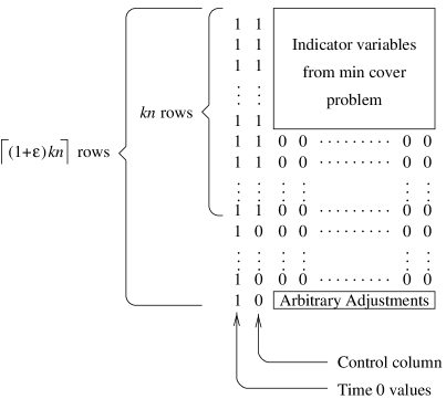
We first show that the required bound is met for the control column if and only if the selected portfolio is made up entirely of rows from the first $kn$ rows (i.e., those rows that contain a 1 in the control column). In particular, the adjustment row may not be included in the portfolio. The market average for the control column is simply

$$\Phi_{1}({\cal M},t)=\frac{kn}{\left\lceil(1+\epsilon)kn\right\rceil}.$$

Obviously, when the portfolio ${\cal M}_{k}$ is made up entirely of these rows, the portfolio average in the control column is 1, so we can bound

$$\frac{\Phi_{1}({\cal M}_{k},t)}{\Phi_{1}({\cal M},t)}=\frac{\left\lceil(1+\epsilon)kn\right\rceil}{kn}\geq 1+\epsilon.$$

On the other hand, when only $k-1$ or fewer of the portfolio rows begin with a 1, then the portfolio average is at most $1-\frac{1}{k}$, and so we can bound

$$\frac{\Phi_{1}({\cal M}_{k},t)}{\Phi_{1}({\cal M},t)} \leq \left(1-\frac{1}{k}\right)\frac{\left\lceil(1+\epsilon)kn\right\rceil}{kn}<\left(1-\frac{1}{k}\right)\frac{(1+\epsilon)kn+1}{kn}$$

$$= \left(1-\frac{1}{k}\right)\left(1+\epsilon+\frac{1}{kn}\right)=1+\epsilon+\frac{1}{kn}-\frac{1}{k}-\frac{\epsilon}{k}-\frac{1}{k^{2}n}$$

$$= 1+\epsilon+-\frac{n-1}{kn}-\frac{\epsilon}{k}-\frac{1}{k^{2}n}<1+\epsilon.$$

Therefore, the desired bound is met only if all $k$ selected rows begin with a 1.

We next show that the desired bound for all other columns is met if and only if at least one row must be selected that contains a non-zero value. If no such rows are selected, all selected rows contain 0 and so the portfolio average is 0. This clearly cannot meet our required bound. On the other hand, if even one row is included with a non-zero value, then $\Phi_{1}({\cal M}_{k},t)\geq\frac{1}{k}$, while the market average for this column is clearly $\frac{n}{\left\lceil(1+\epsilon)kn\right\rceil}$. This leads to

$$\frac{\Phi_{1}({\cal M}_{k},t)}{\Phi_{1}({\cal M},t)}\geq\frac{1}{k}\,\frac{\left\lceil(1+\epsilon)kn\right\rceil}{n}\geq 1+\epsilon,$$

and so the desired bound is met. We note that in order to meet the desired bound on all columns, the adjustment row must not be selected, and therefore the non-zero value required in each column of the portfolio must come from the indicator variables of the original set cover problem. Therefore, an acceptable portfolio exists if and only if an acceptable set cover exists.

References

- [1] G. J. Alexander, W. F. Sharpe, and J. V. Bailey, Fundamentals of Investments, Prentice-Hall, Upper Saddle River, NJ, 2nd ed., 1993.
- [2] T. M. Cover, Universal portfolios, Mathematical Finance, 1 (1991), pp. 1–29.
- [3] T. M. Cover and E. Ordentlich, Universal portfolios with side information, IEEE Transactions on Information Theory, 42 (1996), pp. 348–363.
- [4] M. R. Garey and D. S. Johnson, Computers and Intractability: A Guide to the Theory of NP-Completeness, W. H. Freeman and Company, New York, 1979.