NAACL’00
A Classification Approach to Word Prediction

Abstract

The eventual goal of a language model is to accurately predict the value of a missing word given its context. We present an approach to word prediction that is based on learning a representation for each word as a function of words and linguistics predicates in its context. This approach raises a few new questions that we address. First, in order to learn good word representations it is necessary to use an expressive representation of the context. We present a way that uses external knowledge to generate expressive context representations, along with a learning method capable of handling the large number of features generated this way that can, potentially, contribute to each prediction. Second, since the number of words “competing” for each prediction is large, there is a need to “focus the attention” on a smaller subset of these. We exhibit the contribution of a “focus of attention” mechanism to the performance of the word predictor. Finally, we describe a large scale experimental study in which the approach presented is shown to yield significant improvements in word prediction tasks.

1 Introduction

The task of predicting the most likely word based on properties of its surrounding context is the archetypical prediction problem in natural language processing (NLP). In many NLP tasks it is necessary to determine the most likely word, part-of-speech (POS) tag or any other token, given its history or context. Examples include part-of speech tagging, word-sense disambiguation, speech recognition, accent restoration, word choice selection in machine translation, context-sensitive spelling correction and identifying discourse markers. Most approaches to these problems are based on n-gram-like modeling. Namely, the learning methods make use of features which are conjunctions of typically (up to) three consecutive words or POS tags in order to derive the predictor.

In this paper we show that incorporating additional information into the learning process is very beneficial. In particular, we provide the learner with a rich set of features that combine the information available in the local context along with shallow parsing information. At the same time, we study a learning approach that is specifically tailored for problems in which the potential number of features is very large but only a fairly small number of them actually participates in the decision. Word prediction experiments that we perform show significant improvements in error rate relative to the use of the traditional, restricted, set of features.

Background

The most influential problem in motivating statistical learning application in NLP tasks is that of word selection in speech recognition [Jelinek, 1998]. There, word classifiers are derived from a probabilistic language model which estimates the probability of a sentence $s$ using Bayes rule as the product of conditional probabilities,

$$Pr(s) \doteq Pr(w_{1},w_{2},\ldots w_{n})=$$

$$\doteq \Pi_{i=1}^{n}Pr(w_{i}|w_{1},\ldots w_{i-1})$$

$$\doteq \Pi_{i=1}^{n}Pr(w_{i}|h_{i})$$

where $h_{i}$ is the relevant history when predicting $w_{i}$. Thus, in order to predict the most likely word in a given context, a global estimation of the sentence probability is derived which, in turn, is computed by estimating the probability of each word given its local context or history. Estimating terms of the form $Pr(w|h)$ is done by assuming some generative probabilistic model, typically using Markov or other independence assumptions, which gives rise to estimating conditional probabilities of n-grams type features (in the word or POS space). Machine learning based classifiers and maximum entropy models which, in principle, are not restricted to features of these forms have used them nevertheless, perhaps under the influence of probabilistic methods [Brill, 1995, Yarowsky, 1994, Ratnaparkhi et al., 1994].

It has been argued that the information available in the local context of each word should be augmented by global sentence information and even information external to the sentence in order to learn better classifiers and language models. Efforts in this directions consists of (1) directly adding syntactic information, as in [Chelba and Jelinek, 1998, Rosenfeld, 1996], and (2) indirectly adding syntactic and semantic information, via similarity models; in this case n-gram type features are used whenever possible, and when they cannot be used (due to data sparsity), additional information compiled into a similarity measure is used [Dagan et al., 1999]. Nevertheless, the efforts in this direction so far have shown very insignificant improvements, if any [Chelba and Jelinek, 1998, Rosenfeld, 1996]. We believe that the main reason for that is that incorporating information sources in NLP needs to be coupled with a learning approach that is suitable for it.

Studies have shown that both machine learning and probabilistic learning methods used in NLP make decisions using a linear decision surface over the feature space [Roth, 1998, Roth, 1999]. In this view, the feature space consists of simple functions (e.g., n-grams) over the the original data so as to allow for expressive enough representations using a simple functional form (e.g., a linear function). This implies that the number of potential features that the learning stage needs to consider may be very large, and may grow rapidly when increasing the expressivity of the features. Therefore a feasible computational approach needs to be feature-efficient. It needs to tolerate a large number of potential features in the sense that the number of examples required for it to converge should depend mostly on the number features relevant to the decision, rather than on the number of potential features.

This paper addresses the two issues mentioned above. It presents a rich set of features that is constructed using information readily available in the sentence along with shallow parsing and dependency information. It then presents a learning approach that can use this expressive (and potentially large) intermediate representation and shows that it yields a significant improvement in word error rate for the task of word prediction.

The rest of the paper is organized as follows. In section 2 we formalize the problem, discuss the information sources available to the learning system and how we use those to construct features. In section 3 we present the learning approach, based on the SNoW learning architecture. Section 4 presents our experimental study and results. In section 4.4 we discuss the issue of deciding on a set of candidate words for each decision. Section 5 concludes and discusses future work.

2 Information Sources and Features

Our goal is to learn a representation for each word in terms of features which characterize the syntactic and semantic context in which the word tends to appear. Our features are defined as simple relations over a collection of predicates that capture (some of) the information available in a sentence.

2.1 Information Sources

Definition 1

Let $s=<w_{1},w_{2},...,w_{n}>$ be a sentence in which $w_{i}$ is the $i$-th word. Let ${\cal I}$ be a collection of predicates over a sentence $s$. IS(s)), the Information source(s) available for the sentence $s$ is a representation of $s$ as a list of predicates $I\in{\cal I}$,

$$IS(s)=\{I_{1}(w_{1_{1}},...w_{1_{i}}),...,I_{k}(w_{k_{1}},...w_{k_{i}})\}.$$

$j_{i}$ is the arity of the predicate $I_{j}$.

Example 2

Let $s$ be the sentence
$<{\tt John,X,at,the,clock,to,see,what,time,it,is}>$ Let ${\cal I}$={word, pos, subj-verb}, with the interpretation that word is a unary predicate that returns the value of the word in its domain; pos is a unary predicate that returns the value of the pos of the word in its domain, in the context of the sentence; ${subj-verb}$ is a binary predicate that returns the value of the two words in its domain if the second is a verb in the sentence and the first is its subject; it returns $\phi$ otherwise. Then,

$$IS(s) = \{word(w_{1})={\tt John},...,word(w_{3})={\tt at},...,$$

$$word(w_{11})={\tt is},pos(w_{4})=DET,...,$$

$${subj-verb}(w_{1},w_{2})=\{{\tt John,X}\}...\}.$$

The IS representation of $s$ consists only of the predicates with non-empty values. E.g., $pos(w_{6})=modal$ is not part of the IS for the sentence above. ${subj-verb}$ might not exist at all in the IS even if the predicate is available, e.g., in The ball was given to Mary.

Clearly the $IS$ representation of $s$ does not contain all the information available to a human reading $s$; it captures, however, all the input that is available to the computational process discussed in the rest of this paper. The predicates could be generated by any external mechanism, even a learned one. This issue is orthogonal to the current discussion.

2.2 Generating Features

Our goal is to learn a representation for each word of interest. Most efficient learning methods known today and, in particular, those used in NLP, make use of a linear decision surface over their feature space [Roth, 1998, Roth, 1999]. Therefore, in order to learn expressive representations one needs to compose complex features as a function of the information sources available. A linear function expressed directly in terms of those will not be expressive enough. We now define a language that allows one to define “types” of features in terms of the information sources available to it.

Definition 3 (Basic Features)

Let $I\in{\cal I}$ be a $k$-ary predicate with range $R$. Denote $w^{k}=(w_{j_{1}},\ldots,w_{j_{k}})$. We define two basic binary relations as follows. For $\alpha\in R$ we define:

$$f(I(w^{k}),\alpha)=\left\{\begin{array}[]{l}1\text{ iff }I(w^{k})=\alpha\\ 0\text{ otherwise}\end{array}\right.$$ (1)

An existential version of the relation is defined by:

$$f(I(w^{k}),x)=\left\{\begin{array}[]{l}1\text{ iff }\exists\alpha\in R\,s.t\,I(w^{k})=\alpha\\ 0\text{ otherwise}\end{array}\right.$$ (2)

Features, which are defined as binary relations, can be composed to yield more complex relations in terms of the original predicates available in IS.

Definition 4 (Composing features)

Let $f_{1},f_{2}$ be feature definitions. Then $f_{and}(f_{1},f_{2})$ $f_{or}(f_{1},f_{2})$ $f_{not}(f_{1})$ are defined and given the usual semantic:

$$f_{and}(f_{1},f_{2}) = \left\{\begin{array}[]{l}1\text{ if }f_{1}=f_{2}=1\\ 0\text{ otherwise}\end{array}\right.$$ (5)

$$f_{or}(f_{1},f_{2}) = \left\{\begin{array}[]{l}1\text{ if }f_{1}=1\text{ or }f_{2}=1\\ 0\text{ otherwise}\end{array}\right.$$ (8)

$$f_{not}(f_{1}) = \left\{\begin{array}[]{l}1\text{ if }f_{1}=0\\ 0\text{ otherwise}\end{array}\right.$$ (11)

In order to learn with features generated using these definitions as input, it is important that features generated when applying the definitions on different ISs are given the same identification. In this presentation we assume that the composition operator along with the appropriate IS element (e.g., Ex. 2, Ex. 9) are written explicitly as the identification of the features. Some of the subtleties in defining the output representation are addressed in [Cumby and Roth, 2000].

2.3 Structured Features

So far we have presented features as relations over $IS(s)$ and allowed for Boolean composition operators. In most cases more information than just a list of active predicates is available. We abstract this using the notion of a structural information source $(SIS(s))$ defined below. This allows richer class of feature types to be defined.

2.4 Structured Instances

Definition 5 (Structural Information Source)

Let $s=<w_{1},w_{2},...,w_{n}>$. SIS(s)), the Structural Information source(s) available for the sentence $s$, is a tuple $(s,E_{1},\ldots,E_{k})$ of directed acyclic graphs with $s$ as the set of vertices and $E_{i}$’s, a set of edges in $s$.

Example 6 (Linear Structure)

The simplest SIS is the one corresponding to the linear structure of the sentence. That is, $SIS(s)=(s,E)$ where $(w_{i},w_{j})\in E$ iff the word $w_{i}$ occurs immediately before $w_{j}$ in the sentence (Figure 1 bottom left part).

In a linear structure $(s=<w_{1},w_{2},...,w_{n}>,E)$, where $E=\{(w_{i},w_{i+1});i=1,\ldots n-1\}$, we define the chain

$$C(w_{j},[l,r])=\{w_{j-l},\ldots,w_{j},\ldots w_{j+r}\}\cap s.$$

We can now define a new set of features that makes use of the structural information. Structural features are defined using the SIS. When defining a feature, the naming of nodes in $s$ is done relative to a distinguished node, denoted $w_{p}$, which we call the focus word of the feature. Regardless of the arity of the features we sometimes denote the feature $f$ defined with respect to $w_{p}$ as $f(w_{p})$.

Definition 7 (Proximity)

Let $SIS(s)=(s,E)$ be the linear structure and let $I\in{\cal I}$ be a $k$-ary predicate with range $R$. Let $w_{p}$ be a focus word and $C=C(w_{p},[l,r])$ the chain around it. Then, the proximity features for $I$ with respect to the chain $C$ are defined as:

$$f_{C}(I(w),\alpha)=\left\{\begin{array}[]{l}1\text{ if }I(w)=\alpha,\alpha\in R,w\in C\\ 0\text{ otherwise}\end{array}\right.$$ (12)

The second type of feature composition defined using the structure is a collocation operator.

Definition 8 (Collocation)

Let $f_{1},\ldots f_{k}$ be feature definitions. $colloc_{C}(f_{1},f_{2},\ldots f_{k})$ is a restricted conjunctive operator that is evaluated on a chain $C$ of length $k$ in a graph. Specifically, let $C=\{w_{j_{1}},w_{j_{2}},\ldots,w_{j_{k}}\}$ be a chain of length $k$ in $SIS(s)$. Then, the collocation feature for $f_{1},\ldots f_{k}$ with respect to the chain $C$ is defined as

$$colloc_{C}(f_{1},\ldots,f_{k})=\left\{\begin{array}[]{l}1\text{ if }\forall i=1,\ldots k,f_{i}(w_{j_{i}})=1\\ 0\text{ otherwise}\end{array}\right.$$ (13)

The following example defines features that are used in the experiments described in Sec. 4.

Example 9

Let $s$ be the sentence in Example 2. We define some of the features with respect to the linear structure of the sentence. The word $X$ is used as the focus word and a chain $[-10,10]$ is defined with respect to it. The proximity features are defined with respect to the predicate word. We get, for example: ${\tt f_{C}(word)=John;f_{C}(word)=at;f_{C}(word)=clock.}$

Collocation features are defined with respect to a chain $[-2,2]$ centered at the focus word $X$. They are defined with respect to two basic features $f_{1},f_{2}$ each of which can be either $f(word,\alpha)$ or $f(pos,\alpha)$. The resulting features include, for example:

$$colloc_{C}(word,word) = \{John-X\};$$

$$colloc_{C}(word,word) = \{X-at\};$$

$$colloc_{C}(word,pos) = \{at-DET\}.$$

2.5 Non-Linear Structure

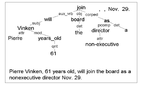
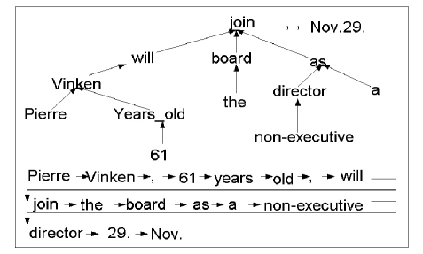
Figure 1: A sentence with a linear and a dependency grammar structure

So far we have described feature definitions which make use of the linear structure of the sentence and yield features which are not too different from standard features used in the literature e.g., $n$-grams with respect to $pos$ or $word$ can be defined as $colloc$ for the appropriate chain. Consider now that we are given a general directed acyclic graph $G=(s,E)$ on the the sentence $s$ as its nodes. Given a distinguished focus word $w_{p}\in s$ we can define a chain in the graph as we did above for the linear structure of the sentence. Since the definitions given above, Def. 7 and Def. 8, were given for chains they would apply for any chain in any graph. This generalization becomes interesting if we are given a graph that represents a more involved structure of the sentence.

Consider, for example the graph $DG(s)$ in Figure 1. $DG(s)$ described the dependency graph of the sentence $s$. An edge $(w_{i},w_{j})$ in $DG(s)$ represent a dependency between the two words. In our feature generation language we separate the information provided by the dependency grammar to two parts. The structural information, provided in the left side of Figure 1, is used to generate $SIS(s)$. The labels on the edges are used as predicates and are part of $IS(s).$ Notice that some authors [Yuret, 1998, Berger and Printz, 1998] have used the structural information, but have not used the information given by the labels on the edges as we do.

The following example defines features that are used in the experiments described in Sec. 4.

Example 10

Let $s$ be the sentence in Figure 1 along with its IS that is defined using the predicates word, pos, subj, obj, aux_vrb. A subj-verb feature, $f_{subj-verb}$, can be defined as a collocation over chains constructed with respect to the focus word join. Moreover, we can define $f_{subj-verb}$ to be active also when there is an aux_vrb between the subj and verb, by defining it as a disjunction of two collocation features, the subj-verb and the subj-aux_vrb-verb. Other features that we use are conjunctions of words that occur before the focus verb (here: join) along all the chains it occurs in (here: will, board, as) and collocations of obj and verb.

As a final comment on feature generation, we note that the language presented is used to define “types” of features. These are instantiated in a data driven way given input sentences. A large number of features is created in this way, most of which might not be relevant to the decision at hand; thus, this process needs to be followed by a learning process that can learn in the presence of these many features.

3 The Learning Approach

Our experimental investigation is done using the SNoW learning system [Roth, 1998]. Earlier versions of SNoW [Roth, 1998, Golding and Roth, 1999, Roth and Zelenko, 1998, Munoz et al., 1999] have been applied successfully to several natural language related tasks. Here we use SNoW for the task of word prediction; a representation is learned for each word of interest, and these compete at evaluation time to determine the prediction.

3.1 The SNOW Architecture

The SNoW architecture is a sparse network of linear units over a common pre-defined or incrementally learned feature space. It is specifically tailored for learning in domains in which the potential number of features might be very large but only a small subset of them is actually relevant to the decision made.

Nodes in the input layer of the network represent simple relations on the input sentence and are being used as the input features. Target nodes represent words that are of interest; in the case studied here, each of the word candidates for prediction is represented as a target node. An input sentence, along with a designated word of interest in it, is mapped into a set of features which are active in it; this representation is presented to the input layer of SNoW and propagates to the target nodes. Target nodes are linked via weighted edges to (some of) the input features. Let $\mathcal{A}_{t}=\{i_{1},\ldots,i_{m}\}$ be the set of features that are active in an example and are linked to the target node $t$. Then the linear unit corresponding to $t$ is active iff

$$\sum_{i\in\mathcal{A}_{t}}w^{t}_{i}>\theta_{t},$$

where $w^{t}_{i}$ is the weight on the edge connecting the $i$th feature to the target node $t$, and $\theta_{t}$ is the threshold for the target node $t$. In this way, SNoW provides a collection of word representations rather than just discriminators.

A given example is treated autonomously by each target subnetwork; an example labeled $t$ may be treated as a positive example by the subnetwork for $t$ and as a negative example by the rest of the target nodes. The learning policy is on-line and mistake-driven; several update rules can be used within SNoW. The most successful update rule is a variant of Littlestone’s Winnow update rule [Littlestone, 1988], a multiplicative update rule that is tailored to the situation in which the set of input features is not known a priori, as in the infinite attribute model [Blum, 1992]. This mechanism is implemented via the sparse architecture of SNoW. That is, (1) input features are allocated in a data driven way – an input node for the feature $i$ is allocated only if the feature $i$ was active in any input sentence and (2) a link (i.e., a non-zero weight) exists between a target node $t$ and a feature $i$ if and only if $i$ was active in an example labeled $t$.

One of the important properties of the sparse architecture is that the complexity of processing an example depends only on the number of features active in it, $n_{a}$, and is independent of the total number of features, $n_{t}$, observed over the life time of the system. This is important in domains in which the total number of features is very large, but only a small number of them is active in each example.

Once target subnetworks have been learned and the network is being evaluated, a decision support mechanism is employed, which selects the dominant active target node in the SNoW unit via a winner-take-all mechanism to produce a final prediction. SNoW is available publicly at http://L2R.cs.uiuc.edu/~cogcomp.html.

4 Experimental Study

4.1 Task definition

The experiments were conducted with four goals in mind:

1. To compare mistake driven algorithms with naive Bayes, trigram with backoff and a simple maximum likelihood estimation (MLE) baseline.

2. To create a set of experiments which is comparable with similar experiments that were previously conducted by other researchers.

3. To build a baseline for two types of extensions of the simple use of linear features: (i) Non-Linear features (ii) Automatic focus of attention.

4. To evaluate word prediction as a simple language model.

We chose the verb prediction task which is similar to other word prediction tasks (e.g.,[Golding and Roth, 1999]) and, in particular, follows the paradigm in [Lee and Pereira, 1999, Dagan et al., 1999, Lee, 1999]. There, a list of the confusion sets is constructed first, each consists of two different verbs. The verb $v_{1\text{ }}$ is coupled with $v_{2}$ provided that they occur equally likely in the corpus. In the test set, every occurrence of $v_{1}$ or $v_{2}$ was replaced by a set $\{v_{1},v_{2}\}$ and the classification task was to predict the correct verb. For example, if a confusion set is created for the verbs ”make” and ”sell”, then the data is altered as follows:

make the paper $$\rightarrow$$ {make,sell}   the paper

sell sensitive data $$\rightarrow$$ {make,sell}   sensitive data

The evaluated predictor chooses which of the two verbs is more likely to occur in the current sentence.

In choosing the prediction task in this way, we make sure the task in difficult by choosing between competing words that have the same prior probabilities and have the same part of speech. A further advantage of this paradigm is that in future experiments we may choose the candidate verbs so that they have the same sub-categorization, phonetic transcription, etc. in order to imitate the first phase of language modeling used in creating candidates for the prediction task. Moreover, the pre-transformed data provides the correct answer so that (i) it is easy to generate training data; no supervision is required, and (ii) it is easy to evaluate the results assuming that the most appropriate word is provided in the original text.

Results are evaluated using word-error rate (WER). Namely, every time we predict the wrong word it is counted as a mistake.

4.2 Data

We used the Wall Street Journal (WSJ) of the years 88-89. The size of our corpus is about 1,000,000 words. The corpus was divided into 80% training and 20% test. The training and the test data were processed by the FDG parser [Tapanainen and J rvinen, 1997]. Only verbs that occur at least 50 times in the corpus were chosen. This resulted in $278$ verbs that we split into $139$ confusion sets as above. After filtering the examples of verbs which were not in any of the sets we use $73,184$ training examples and $19,852$ test examples.

4.3 Results

4.3.1 Features

In order to test the advantages of different feature sets we conducted experiments using the following features sets:

1. Linear features: proximity of window size $\pm 10$ words, conjunction of size 2 using window size $\pm 2$. The conjunction combines words and parts of speech.

2. Linear + Non linear features: using the linear features defined in (1) along with non linear features that use the predicates subj, obj, word, pos, the collocations subj-verb, verb-obj linked to the focus verb via the graph structure and conjunction of $2$ linked words.

The over all number of features we have generated for all $278$ target verbs was around $400,000$. In all tables below the NB columns represent results of the naive Bayes algorithm as implemented within SNoW and the SNoW column represents the results of the sparse Winnow algorithm within SNoW.

	Bline	NB	SNoW
Linear	$49.6$	$13.54$	$11.56$
Non Linear	$49.6$	$12.25$	$9.84$

Table 1: Word Error Rate results for linear and non-linear features

Table 1 summarizes the results of the experiments with the features sets (1), (2) above. The baseline experiment uses MLE, the majority predictor. In addition, we conducted the same experiment using trigram with backoff and the WER is $29.3\%$. From these results we conclude that using more expressive features helps significantly in reducing the WER. However, one can use those types of features only if the learning method handles large number of possible features. This emphasizes the importance of the new learning method.

	Similarity	NB	SNoW
WSJ data		$54.6\%$	$59.1\%$
AP news	$47.6\%$

Table 2: Comparison of the improvement achieved using similarity methods [Dagan et al., 1999] and using the methods presented in this paper. Results are shown in percentage of improvement in accuracy over the baseline.

Table 2 compares our method to methods that use similarity measures [Dagan et al., 1999, Lee, 1999]. Since we could not use the same corpus as in those experiments, we compare the ratio of improvement and not the WER. The baseline in this studies is different, but other than that the experiments are identical. We show an improvement over the best similarity method. Furthermore, we train using only $73,184$ examples while [Dagan et al., 1999] train using $587,833$ examples. Given our experience with our approach on other data sets we conjecture that we could have improved the results further had we used that many training examples.

4.4 Focus of attention

SNoW is used in our experiments as a multi-class predictor - a representation is learned for each word in a given set and, at evaluation time, one of these is selected as the prediction. The set of candidate words is called the confusion set [Golding and Roth, 1999]. Let $C$ be the set of all target words. In previous experiments we generated artificially subsets of size $2$ of $C$ in order to evaluate the performance of our methods. In general, however, the question of determining a good set of candidates is interesting in it own right. In the absence of a good method, one might end up choosing a verb from among a larger set of candidates. We would like to study the effects this issue has on the performance of our method.

In principle, instead of working with a single large confusion set $C$, it might be possible to split $C$ into subsets of smaller size. This process, which we call the focus of attention (FOA) would be beneficial only if we can guarantee that, with high probability, given a prediction task, we know which confusion set to use, so that the true target belongs to it. In fact, the FOA problem can be discussed separately for the training and test stages.

1. Training: Given our training policy (Sec. 3) every positive example serves as a negative example to all other targets in its confusion set. For a large set $C$ training might become computationally infeasible.

2. Testing: considering only a small set of words as candidates at evaluation time increases the baseline and might be significant from the point of view of accuracy and efficiency.

To evaluate the advantage of reducing the size of the confusion set in the training and test phases, we conducted the following experiments using the same features set (linear features as in Table 1).

	Bline	NB	SNoW
Train All Test All	$87.44$	$65.22$	$65.05$
Train All Test 2	$49.6$	$13.54$	$13.15$
Train 2 Test 2	$49.6$	$13.54$	$11.55$

Table 3: Evaluating Focus of Attention: Word Error Rate for Training and testing using all the words together against using pairs of words.

“Train All” means training on all 278 targets together. “Test all” means that the confusion set is of size 278 and includes all the targets. The results shown in Table 3 suggest that, in terms of accuracy, the significant factor is the confusion set size in the test stage. The effect of the confusion set size on training is minimal (although it does affect training time). We note that for the naive Bayes algorithm the notion of negative examples does not exist, and therefore regardless of the size of confusion set in training, it learns exactly the same representations. Thus, in the NB column, the confusion set size in training makes no difference.

The application in which a word predictor is used might give a partial solution to the FOA problem. For example, given a prediction task in the context of speech recognition the phonemes that constitute the word might be known and thus suggest a way to generate a small confusion set to be used when evaluating the predictors.

Tables 4,5 present the results of using artificially simulated speech recognizer using a method of general phonetic classes. That is, instead of transcribing a word by the phoneme, the word is transcribed by the phoneme classes[Jurafsky and Martin, 200]. Specifically, these experiments deviate from the task definition given above. The confusion sets used are of different sizes and they consist of verbs with different prior probabilities in the corpus. Two sets of experiments were conducted that use the phonetic transcription of the words to generate confusion sets.

	Bline	NB	SNoW
Train All Test PC	19.84	11.6	12.3
Train PC Test PC	19.84	11.6	11.3

Table 4: Simulating Speech Recognizer: Word Error Rate for Training and testing with confusion sets determined based on phonetic classes (PC) from a simulated speech recognizer.

In the first experiment (Table 4), the transcription of each word is given by the broad phonetic groups to which the phonemes belong i.e., nasals, fricative, etc.. For example, the word ”b_u_y” is transcribed using phonemes as ”b_Y” and here we transcribe it as ”P_V1” which stands for ”Plosive_Vowel1”. This partition results in a partition of the set of verbs into several confusions sets. A few of these confusion sets consist of a single word and therefore have 100% baseline, which explains the high baseline.

	Bline	NB	SNoW
Train All Test PC	45.63	26.36	27.54
Train PC Test PC	45.63	26.36	25.55

Table 5: Simulating Speech Recognizer: Word Error Rate for Training and testing with confusion sets determined based on phonetic classes (PC) from a simulated speech recognizer. In this case only confusion sets that have less than 98% baseline are used, which explains the overall lower baseline.

Table 5 presents the results of a similar experiment in which only confusion sets with multiple words were used, resulting in a lower baseline.

As before, Train All means that training is done with all 278 targets together while Train PC means that the PC confusion sets were used also in training. We note that for the case of SNoW, used here with the sparse Winnow algorithm, that size of the confusion set in training has some, although small, effect. The reason is that when the training is done with all the target words, each target word representation with all the examples in which it does not occur are used as negative examples. When a smaller confusion set is used the negative examples are more likely to be “true” negative.

5 Conclusion

This paper presents a new approach to word prediction tasks. For each word of interest, a word representation is learned as a function of a common, but potentially very large set of expressive (relational) features. Given a prediction task (a sentence with a missing word) the word representations are evaluated on it and compete for the most likely word to complete the sentence.

We have described a language that allows one to define expressive feature types and have exhibited experimentally the advantage of using those on word prediction task. We have argued that the success of this approach hinges on the combination of using a large set of expressive features along with a learning approach that can tolerate it and converges quickly despite the large dimensionality of the data. We believe that this approach would be useful for other disambiguation tasks in NLP.

We have also presented a preliminary study of a reduction in the confusion set size and its effects on the prediction performance. In future work we intend to study ways that determine the appropriate confusion set in a way to makes use of the current task properties.

Acknowledgments

We gratefully acknowledge helpful comments and programming help from Chad Cumby.

References

- Berger and Printz, 1998 A. Berger and H. Printz. 1998. Recognition performance of a large-scale dependency-grammar language model. In Int’l Conference on Spoken Language Processing (ICSLP’98), Sydney, Australia.
- Blum, 1992 A. Blum. 1992. Learning boolean functions in an infinite attribute space. Machine Learning, 9(4):373–386.
- Brill, 1995 E. Brill. 1995. Transformation-based error-driven learning and natural language processing: A case study in part of speech tagging. Computational Linguistics, 21(4):543–565.
- Chelba and Jelinek, 1998 C. Chelba and F. Jelinek. 1998. Exploiting syntactic structure for language modeling. In COLING-ACL’98.
- Cumby and Roth, 2000 C. Cumby and D. Roth. 2000. Relational representations that facilitate learning. In Proc. of the International Conference on the Principles of Knowledge Representation and Reasoning. To appear.
- Dagan et al., 1999 I. Dagan, L. Lee, and F. Pereira. 1999. Similarity-based models of word cooccurrence probabilities. Machine Learning, 34(1-3):43–69.
- Golding and Roth, 1999 A. R. Golding and D. Roth. 1999. A Winnow based approach to context-sensitive spelling correction. Machine Learning, 34(1-3):107–130. Special Issue on Machine Learning and Natural Language.
- Jelinek, 1998 F. Jelinek. 1998. Statistical Methods for Speech Recognition. MIT Press.
- Jurafsky and Martin, 200 D. Jurafsky and J. H. Martin. 200. Speech and Language Processing. Prentice Hall.
- Lee and Pereira, 1999 L. Lee and F. Pereira. 1999. Distributional similarity models: Clustering vs. nearest neighbors. In ACL 99, pages 33–40.
- Lee, 1999 L. Lee. 1999. Measure of distributional similarity. In ACL 99, pages 25–32.
- Littlestone, 1988 N. Littlestone. 1988. Learning quickly when irrelevant attributes abound: A new linear-threshold algorithm. Machine Learning, 2:285–318.
- Munoz et al., 1999 M. Munoz, V. Punyakanok, D. Roth, and D. Zimak. 1999. A learning approach to shallow parsing. In EMNLP-VLC’99, the Joint SIGDAT Conference on Empirical Methods in Natural Language Processing and Very Large Corpora, June.
- Ratnaparkhi et al., 1994 A. Ratnaparkhi, J. Reynar, and S. Roukos. 1994. A maximum entropy model for prepositional phrase attachment. In ARPA, Plainsboro, NJ, March.
- Rosenfeld, 1996 R. Rosenfeld. 1996. A maximum entropy approach to adaptive statistical language modeling. Computer, Speech and Language, 10.
- Roth and Zelenko, 1998 D. Roth and D. Zelenko. 1998. Part of speech tagging using a network of linear separators. In COLING-ACL 98, The 17th International Conference on Computational Linguistics, pages 1136–1142.
- Roth, 1998 D. Roth. 1998. Learning to resolve natural language ambiguities: A unified approach. In Proc. National Conference on Artificial Intelligence, pages 806–813.
- Roth, 1999 D. Roth. 1999. Learning in natural language. In Proc. of the International Joint Conference of Artificial Intelligence, pages 898–904.
- Tapanainen and J rvinen, 1997 P. Tapanainen and T. J rvinen. 1997. A non-projective dependency parser. In In Proceedings of the 5th Conference on Applied Natural Language Processing, Washington DC.
- Yarowsky, 1994 D. Yarowsky. 1994. Decision lists for lexical ambiguity resolution: application to accent restoration in Spanish and French. In Proc. of the Annual Meeting of the ACL, pages 88–95.
- Yuret, 1998 D. Yuret. 1998. Discovery of Linguistic Relations Using Lexical Attraction. Ph.D. thesis, MIT.